pdf file 10.5 MB - ISSI
pdf file 10.5 MB - ISSI
pdf file 10.5 MB - ISSI

Create successful ePaper yourself
Turn your PDF publications into a flip-book with our unique Google optimized e-Paper software.
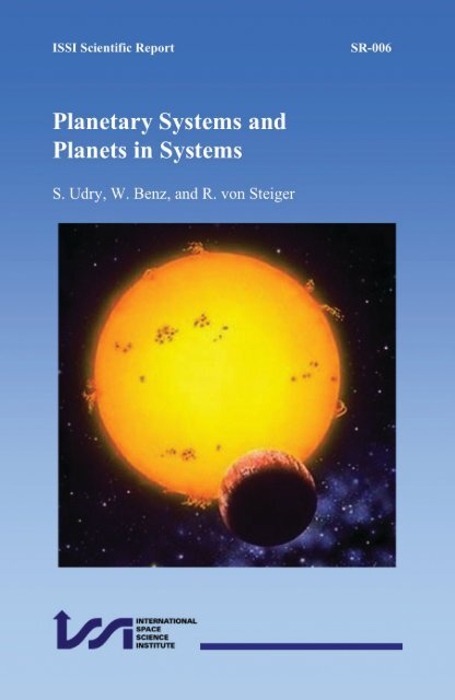
SR-006<br />
December 2006<br />
Planetary Systems and<br />
Planets in Systems<br />
Editors<br />
Stephane Udry<br />
Observatoire de Genève, Sauverny, Switzerland<br />
Willy Benz<br />
Physikalisches Institut, University of Bern, Switzerland<br />
Rudolf von Steiger<br />
International Space Science Institute, Bern, Switzerland<br />
Dedicated to Michel Mayor on the occasion of his 60 th birthday<br />
PlanetarySystems.tex; 28/12/2006; 12:00; p.1
ii<br />
Cover: Artists impression of a transiting extrasolar planet. From obswww.unige.<br />
ch/˜udry/planet/planet.html<br />
The International Space Science Institute is a Foundation under Swiss law. It is<br />
funded by the European Space Agency, the Swiss Confederation, the Swiss National<br />
Science Foundation, and the University of Bern.<br />
Published for:<br />
The International Space Science Institute<br />
Hallerstrasse 6, CH-3012 Bern, Switzerland<br />
by:<br />
ESA Publications Division<br />
Keplerlaan 1, 2200 AG Noordwijk, The Netherlands<br />
Publication Manager:<br />
Cover Design:<br />
Bruce Battrick<br />
N.N.<br />
Copyright:<br />
ISSN:<br />
Price:<br />
c○2006 <strong>ISSI</strong>/ESA<br />
ZZZZ-YYYX<br />
XX Euros<br />
PlanetarySystems.tex; 28/12/2006; 12:00; p.2
iii<br />
Contents<br />
Foreword................................................................v<br />
Michel Mayor, Science with Enthusiasm and Humour<br />
A. Maeder ...............................................................vi<br />
I: Giant Planets: General View<br />
Chemical Properties of Stars with Giant Planets<br />
N. C. Santos, M. Mayor, and G. Israelian ....................................3<br />
Current Challenges Facing Planet Transit Surveys<br />
D. Charbonneau .........................................................17<br />
Angular Momentum Constraints on Type II Planet Migration<br />
W. R. Ward ..............................................................29<br />
On Multiple Planet Systems<br />
W. Kley .................................................................39<br />
A New Constraint on the Formation of Jupiter<br />
T. Owen ................................................................51<br />
II: Multi-Planetary Systems: Observations<br />
Isotopic Constraints on the Formation of Earth-Like Planets<br />
A. N. Halliday ...........................................................59<br />
Planets Around Neutron Stars<br />
A. Wolszczan ............................................................77<br />
Systems of Multiple Planets<br />
G. W. Marcy, D. A. Fischer, R. P. Butler, and S. S. Vogt .......................89<br />
Debris Disks<br />
A.-M. Lagrange and J.-C. Augereau ......................................105<br />
III: Multi-Planetary Systems: Theory<br />
Formation of Cores of Giant Planets and an Implication for “Planet Desert”<br />
S. Ida..................................................................115<br />
Chaotic Interactions in Multiple Planet Systems<br />
E. B. Ford, F. A. Rasio, and K. Yu.........................................123<br />
Disc Interactions Resonances and Orbital Relaxation in Extrasolar Planetary Systems<br />
J. C. B. Papaloizou, R. P. Nelson, and C. Terquem ..........................137<br />
PlanetarySystems.tex; 28/12/2006; 12:00; p.3
iv<br />
IV: Planets in Systems<br />
Properties of Planets in Binaries<br />
S. Udry, A. Eggenberger, and M. Mayor ...................................157<br />
On the Formation and Evolution of Giant Planets in Close Binary Systems<br />
R. P. Nelson ............................................................171<br />
Induced Eccentricities of Extra Solar Planets by Distant Stellar Companions<br />
T. Mazeh...............................................................185<br />
Is Planetary Migration Inevitable?<br />
C. Terquem ............................................................195<br />
V: Missions<br />
The Kepler Mission<br />
W.Boruckietal.........................................................205<br />
The Exoplanet Program of the CoRoT Space Mission<br />
C. Moutou and the CoRoT Team .........................................219<br />
VI: Working Group Reports<br />
Report of the Working Group on Detection Methods<br />
T. M. Brown and J.-R. De Medeiros.......................................225<br />
Dynamical Interactions Among Extrasolar Planets and their Observability in Radial<br />
Velocity Data Sets<br />
G. Laughlin and J. Chambers ............................................231<br />
VII: Future and Conclusions<br />
Theories of Planet Formation: Future Prospects<br />
J. J. Lissauer ...........................................................247<br />
Direct Detection Of Exoplanets: A Dream or a Near-Future Reality?<br />
D. Rouan ..............................................................261<br />
Planets With Detectable Life<br />
T. Owen ...............................................................277<br />
Outlook: Testing Planet Formation Theories<br />
A. P. Boss ..............................................................285<br />
PlanetarySystems.tex; 28/12/2006; 12:00; p.4
v<br />
Foreword<br />
Sometext...<br />
Bern, December 2006<br />
Stephane Udry, Willy Benz, Rudolf von Steiger<br />
PlanetarySystems.tex; 28/12/2006; 12:00; p.5
vi<br />
PlanetarySystems.tex; 28/12/2006; 12:00; p.6
vii<br />
Michel Mayor, Science with Enthusiasm and Humour<br />
Michel Mayor joined the Geneva Observatory as an assistant in 1965. Throughout<br />
his career he has always shown the juvenile curiosity that we know for interesting<br />
questions in astrophysics and science in general. All kinds of questions, from scientific<br />
to social and political ones, with him are a matter for lively discussions, not<br />
without a good touch of humour. These interests go along with a visionary intuition<br />
and perseverance, necessary to make great achievements. Scientific questions do<br />
not prevent Michel to like climbing on mountains and travelling around the world.<br />
I must also add that Michel has the pleasant conviviality which allowed people to<br />
have nice lunches together, full of laughters and jokes, at the Observatory most<br />
weekdays during forty years.<br />
Back in 1969, in the first volume of the newborn journal Astronomy & Astrophysics,<br />
there was an article by Michel Mayor and Louis Martinet. The subject<br />
was already “motions”, not yet motions of planets, but of nearby stars in relation<br />
with ages and stellar properties. These researches in galactic dynamics culminated<br />
in a study with Laurent Vigroux in 1981 on the effects of matter infalling on the<br />
Galaxy with zero angular momentum. Indeed, the studies of motions of astronomical<br />
objects is the basic “red line” of all Michel’s researches. Like all astronomers<br />
who wanted to have some chance to stay at Geneva Observatory, Michel had to<br />
perform some mandatory photometric missions in Haute-Provence. Around 1968,<br />
everything which might more or less resemble to student contests would be regarded<br />
with suspicion at Observatory. I remember when Michel, with new familial<br />
responsibilities, once asked the administrator what his wife and children would<br />
receive as indemnity in case of decease. The administrator, who was nevertheless a<br />
nice man, went furious through the institute shouting “These assistants! They want<br />
all advantages for themselves”.<br />
At the end of the seventies, Michel Mayor had developed, in collaboration with<br />
André Baranne, the Coravel spectrograph with the basic idea to study the stellar<br />
dynamics in the Galaxy by means of radial velocities. Coravel turned out to be<br />
most useful for many original studies, like stellar rotation of low mass stars with<br />
Willy Benz and later with José de Medeiros for evolved stars, Cepheids and binaries<br />
with Gilbert Burki and later with Antoine Duquennoy and globular clusters<br />
with Georges Meylan. In order to improve the accuracy of radial velocities, the<br />
Elodie spectrograph was developed in the early nineties. The main objective of the<br />
observing programme was brown dwarfs and planetary companions. Today, it may<br />
look unbelievable that only ten years ago the subject of planets was not a topical<br />
one, even worse it was even a “dusty” and often not well perceived topic. Thus,<br />
when they realized that the accuracy was perhaps enough to try to find planets,<br />
PlanetarySystems.tex; 28/12/2006; 12:00; p.7
viii<br />
Michel Mayor and Didier Queloz in an application for observing time only speak<br />
about brown dwarfs and possible “sub-stellar” objects in the title of their proposal.<br />
The historical discovery of the first extra-solar planet around 51 Pegasi in 1995<br />
by Michel and Didier immediately had a great impact in the astronomical community<br />
and by the public as well. As often in Switzerland, the discovery became well<br />
recognized locally by the media when it was subsequently confirmed by Americans.<br />
The finding of extra-solar planets brought a kind of “Planetary Revolution” in<br />
Astronomy and placed the planets among the most topical scientific researches and<br />
the most popular ones. Exobiology and the search for extraterrestrial life have then<br />
become much more respectable. This deep change of minds, which leads to both<br />
new theoretical developments and major space programmes, is most impressive.<br />
All started out or was strongly boosted by the discovery of 51 Pegasi.<br />
The golden age of discoveries continues today, new extrasolar planets are announced<br />
regularly which has stirred international collaboration and sometimes also<br />
competition. Michel and his team, with the efficient collaboration of Stéphane<br />
Udry, Nuno Santos, Dominique Naef and others not only go on at a leading place<br />
in planetary search, but also develops great projects for the future. The new spectrograph<br />
Harps, achieved in cooperation with ESO thanks to the competence of<br />
Francesco Pepe, reaches the amazing accuracy of about 30 cm/s. It opens up fascinating<br />
perspectives in planetary search and asteroseismology.<br />
Since about forty years, Michel and myself have been colleagues and nevertheless<br />
good friends, going through various steps in the responsibilities at the Geneva<br />
Observatory, as assistants under the chairmanship of Marcel Golay, research associates,<br />
professors and even more recently as successive directors of the Geneva<br />
Observatory. In the name of all colleagues and friends in Geneva and abroad, I<br />
address to Michel our warm congratulations and best wishes for the future. Our<br />
compliments are also for Françoise Mayor, who among other qualities has a great<br />
sense of the real relative importance of things in life.<br />
At the age of sixty, Michel, keep on going like you did over all this time, as a<br />
friendly colleague, keeping good health and scientific enthusiasm!<br />
Geneva Observatory, October 20, 2003<br />
André Maeder<br />
PlanetarySystems.tex; 28/12/2006; 12:00; p.8
ix<br />
PlanetarySystems.tex; 28/12/2006; 12:00; p.9
x<br />
PlanetarySystems.tex; 28/12/2006; 12:00; p.10
Part I<br />
Giant Planets: General View<br />
PlanetarySystems.tex; 28/12/2006; 12:00; p.11
PlanetarySystems.tex; 28/12/2006; 12:00; p.12
Chemical Properties of Stars with Giant Planets<br />
N. C. Santos and M. Mayor<br />
Observatoire de Genève, CH-1290 Sauverny, Switzerland<br />
G. Israelian<br />
Instituto de Astrofísica de Canarias, E-38200 La Laguna, Tenerife, Spain<br />
Abstract. In this paper we review the current situation regarding the study of the metallicity-giant<br />
planet connection. We show that planet-host stars are more metal-rich than average field dwarfs, a<br />
trend that remains after the discovery of now more than about 100 planets. Current results also point<br />
out that the planetary frequency is rising as a function of the [Fe/H]. Furthermore, the source of this<br />
high metallicity is shown to have most probably an “original” source, although there are also some<br />
evidences for stellar “pollution”. These facts seem to be telling us that the metallicity is playing a very<br />
important role in the formation of the now discovered giant planets. We further compare the orbital<br />
properties (minimum mass, period and eccentricity) of planet hosts with their chemical abundances.<br />
Some slight trends are seen and discussed.<br />
1. Introduction<br />
The last few years have been very prolific regarding the research for new planetary<br />
systems. Following the discovery of the planetary companion to the solar-type<br />
star 51 Peg (Mayor and Queloz, 1995), more than 100 extra-solar giant planets<br />
are known today 1 . These results opened a wide range of questions regarding the<br />
understanding of the mechanisms of planetary formation.<br />
To find a solution for the many problems risen, we need observational constraints.<br />
These can come, for example, from the analysis of the orbital parameters<br />
of the known planets, like the distribution of planetary masses, eccentricities, or<br />
orbital periods (see contribution from Mayor et al. in this volume). But further<br />
evidences are coming from the study of the planet host stars themselves. Precise<br />
spectroscopic studies have revealed that stars with planets seem to be particularly<br />
metal-rich when compared with “single” field dwarfs (Gonzalez, 1997; Santos et<br />
al., 2001). Furthermore, the frequency of planets seems to be a strong function of<br />
[Fe/H] (Santos et al., 2001). These facts, that were shown not to result from any<br />
sampling bias, are most probably telling us that the metallicity plays a key role in<br />
the formation of a giant planet, or at least of the giant planets like the ones we are<br />
finding now.<br />
The nature of the metallicity-giant planet connection has been strongly debated<br />
in the literature. Some authors have suggested that the high metal content of the<br />
1 See http://obswww.unige.ch/exoplanets. Before 1995 only planets around a pulsar<br />
had been detected (Wolszczan and Frail, 1992); these are probably second generation planets.<br />
Also, the previously discovered radial-velocity companion around HD 114762 (Latham et al., 1989)<br />
has a minimum mass above 10M Jup , and is likely a brown-dwarf<br />
PlanetarySystems.tex; 28/12/2006; 12:00; p.13
4 N. C. Santos et al.<br />
Figure 1. Left: metallicity distribution for stars with planets (hashed histogram) compared with the<br />
same distribution for the field dwarfs (empty histogram). The vertical lines represent stars with brown<br />
dwarf candidate companions. Right: The cumulative functions of both samples. A Kolmogorov-Smirnov<br />
test shows the probability for the two populations being part of the same sample is around<br />
10 −7 . From Santos et al. (2002b).<br />
planet host stars may have an external origin: it results from the addition of metalrich<br />
(hydrogen poor) material into the convective envelope of the star, a process<br />
that could result from the planetary formation process itself (Gonzalez, 1998). Evidences<br />
for the infall of planetary material have in fact been found for a few planet<br />
host stars (Israelian et al., 2001; Laws and Gonzalez, 2001; Israelian et al., 2002),<br />
although not necessarily able to change considerably their overall metal content.<br />
In fact, most evidences today suggest that the metallicity “excess” as a whole has<br />
a “primordial” origin (Pinsonneault et al., 2001; Santos et al., 2001; Santos et al.,<br />
2003), and thus that the metal content of the cloud giving birth to the star and<br />
planetary system is indeed a key parameter to form a giant planet.<br />
In this article we will make a review of the current situation regarding the results<br />
obtained in the context of the study of the metallicity of planet-host stars. Most of<br />
the results presented here were published in Santos et al. (2001) and Santos et al.<br />
(2003), for which we refer for more details.<br />
2. The Metallicity of Planet Host Stars<br />
In Figure 1 we plot the metallicity distribution for all the stars known to have<br />
companions with minimum masses lower than ∼ 18M Jup (hashed histogram) when<br />
compared to the same distribution for a volume limited sample of stars with no<br />
(known) planetary companions (open histogram) – see Santos et al. (2001). For the<br />
planet host stars, most of the metallicity values ([Fe/H]) were taken from Santos et<br />
al. (2001) and Santos et al. (2003). It is important to remember that the metallicity<br />
PlanetarySystems.tex; 28/12/2006; 12:00; p.14
Chemical Properties of Stars with Giant Planets 5<br />
Figure 2. Plot of the mean-photon noise error for the CORALIE measurements of stars having<br />
magnitude V between 6 and 7, as a function of the metallicity. Most planet host stars present<br />
radial-velocity variations with an amplitude larger than 30 m s −1 (dotted line). From Santos et al.<br />
(2002).<br />
for the two samples of stars plotted in Figure 1 was derived using exactly the same<br />
method, and are thus both in the same scale.<br />
As is clearly visible in the figures, stars with planetary companions are more<br />
metal-rich (in average) than field dwarfs. The average metallicity difference between<br />
the two samples is about 0.22 dex, and the probability that the two distributions<br />
belong to the same sample is of the order of 10 −7 .<br />
In the figure, stars having planetary companions with masses higher than 10M Jup<br />
are denoted by the vertical lines. Given the still low number, it is impossible to do<br />
any statistical study of this group. However, up to now there does not seem to exist<br />
any clear difference between the two populations.<br />
2.1. NO METALLICITY BIAS<br />
Particular concern has been shown by the community regarding the fact that a<br />
higher metallicity will imply that the spectral lines are better defined. This could<br />
mean that the final precision in radial-velocity could be better for the more “metallic”<br />
objects, leading thus to an increasing detection rate as a function of increasing<br />
[Fe/H].<br />
PlanetarySystems.tex; 28/12/2006; 12:00; p.15
6 N. C. Santos et al.<br />
In Figure 2 we plot the mean photon noise error for stars with different [Fe/H]<br />
having V magnitudes between 6 and 7. As we can see, there is no particularly<br />
important trend in the data. The very slight tendency (metal-rich stars have, in<br />
average, measurements with only about 1–2 m s −1 better precision than metal poor<br />
stars) is definitely not able to induce the strong tendency seen in the [Fe/H] distribution<br />
of planet host stars, specially when we compare it with the usual velocity<br />
amplitude induced by the known planetary companions (a few tens of meters-persecond).<br />
In fact, in the CORALIE survey we always set the exposure times in order to<br />
have approximately the same photon-noise error. This also seems to be the case<br />
concerning the Lick/Keck planet search programs (D. Fischer, private communication).<br />
2.2. THE SOURCE OF THE METALLICITY<br />
Two different interpretations have been given to the [Fe/H] “excess” observed for<br />
stars with planets. One suggests that the high metal content is the result of the<br />
accretion of planets and/or planetary material into the star (e.g. Gonzalez, 1998).<br />
Another simply states that the planetary formation mechanism is dependent on<br />
the metallicity of the proto-planetary disk: according to the “traditional” view, a<br />
gas giant planet is formed by runaway accretion of gas by a ∼10 earth masses<br />
planetesimal (Pollack et al., 2001). The higher the metallicity (and thus the number<br />
of dust particles) the faster a planetesimal can grow, and the higher the probability<br />
of forming a giant planet before the gas in the disk dissipates.<br />
There are multiple ways of deciding between the two scenarios. Probably the<br />
most clear and strong argument is based on stellar internal structure, in particular on<br />
the fact that material falling into a star’s surface would induce a different increase<br />
in [Fe/H] depending on the stellar mass, i.e. on the depth of its convective envelope<br />
(where mixing can occur). However, the data shows no such trend (Figure 3) –<br />
(Santos et al., 2001; Santos et al., 2003). In particular, a quick look at the plot indicates<br />
that the upper envelope of the points is quite constant. A similar conclusion<br />
was also recently taken by Pinsonneault et al. (2001) that showed that even nonstandard<br />
models of convection and diffusion cannot explain the lack of a trend and<br />
sustain “pollution” as the source of the high-[Fe/H].<br />
Together with the similarity of [Fe/H] abundances for dwarf and sub-giant planet<br />
host stars 2 (Santos et al., 2001; Santos et al., 2003), the facts presented here strongly<br />
suggest a “primordial origin” to the high-metal content of stars with giant planets.<br />
This result implies that the metallicity is a key parameter controlling planet formation<br />
and evolution, and may have enormous implications on theoretical models.<br />
2 These latter are supposed to have diluted already any strong metallicity excess present, since<br />
their convective envelopes have deepened as a result of stellar evolution<br />
PlanetarySystems.tex; 28/12/2006; 12:00; p.16
Chemical Properties of Stars with Giant Planets 7<br />
Figure 3. Metallicity vs. convective envelope mass for stars with planets (open symbols) and field<br />
dwarfs (points). The [Fe/H]=constant line represents the mean [Fe/H] for the non-planet hosts stars<br />
of Figure 1. The curved line represents the result of adding 8 earth masses of iron to the convective<br />
envelope of stars having an initial metallicity equal to the non-planet hosts mean [Fe/H]. The resulting<br />
trend has no relation with the distribution of the stars with planets. From Santos et al. (2002b).<br />
2.3. THE FREQUENCY OF PLANETARY FORMATION<br />
In Figure 4 (left panel) we plot the [Fe/H] distribution for a large volume limited<br />
sample of stars included in the CORALIE survey (Udry et al., 2000) 3 when compared<br />
with the same distribution for planet host stars that belong to the CORALIE<br />
planet-search sample itself.<br />
The knowledge of the metallicity distribution for stars in the solar neighborhood<br />
(and included in the CORALIE sample) permits us to determine the percentage of<br />
planet host stars per metallicity bin. This analysis is presented in Figure 4 (right<br />
panel). As we can perfectly see, the probability of finding a planet host is a strong<br />
function of its metallicity. For example, about 7% of the stars in the CORALIE<br />
sample having metallicity between 0.3 and 0.4 dex have been discovered to harbor a<br />
planet. On the other hand, less than 1% of the stars having solar metallicity seem to<br />
have a planet. This result is thus probably telling us that the probability of forming<br />
a giant planet, or at least a planet of the kind we are finding now, depends strongly<br />
on the metallicity of the gas that gave origin to the star and planetary system.<br />
3 The metallicities for this sample were computed from a precise calibration of the CORALIE<br />
Cross-Correlation Function (Santos et al., 2002a)<br />
PlanetarySystems.tex; 28/12/2006; 12:00; p.17
8 N. C. Santos et al.<br />
Figure 4. Left: metallicity distribution of stars with planets making part of the CORALIE planet<br />
search sample (shaded histogram) compared with the same distribution for the about 1000 non<br />
binary stars in the CORALIE volume-limited sample (see text for more details). Right: theresult<br />
of correcting the planet hosts distribution to take into account the sampling effects. The vertical axis<br />
represents the percentage of planet hosts with respect to the total CORALIE sample. From Santos et<br />
al. (2002b).<br />
This result seems to be telling us that the planetary formation efficiency (at least<br />
of the kind of planets we are finding now) is a strong function of the metallicity.<br />
It is important to discuss the implications of this result on the planetary formation<br />
scenarios. Boss (2002) has shown that in the core accretion scenario we<br />
can expect the efficiency of planetary formation to be strongly dependent on the<br />
metallicity, contrarily of what could be expected from a mechanism of disk instability.<br />
The results presented here, suggesting that the probability of forming a<br />
planet is strongly dependent on the metallicity of the host star, can thus be seen<br />
as an argument for the former (traditional) core accretion scenario (Pollack et al.,<br />
2001). We note that here we are talking about a probabilistic effect: the fact that<br />
the metallicity enhances the probability of forming a planet does not mean one<br />
cannot for a planet in a lower metallicity environment. This might be due to the fact<br />
that other important and unknown parameters, like the proto-planetary disk mass<br />
and lifetime, do control the efficiency of planetary formation as well. Furthermore,<br />
these results do not exclude that an overlap might exist between the two planetary<br />
formation scenarios.<br />
3. Metallicity and Orbital Parameters<br />
Some hints of trends between the metallicity of the host stars and the orbital parameters<br />
of their planets have been discussed already in the literature. The usually<br />
low number of points involved in the statistics did not permit, however, to extract<br />
PlanetarySystems.tex; 28/12/2006; 12:00; p.18
Chemical Properties of Stars with Giant Planets 9<br />
Figure 5. Left: [Fe/H] distributions for planets orbiting with periods shorter and higher than 10<br />
days (the hashed and open bars, respectively). Right: cumulative functions of both distributions.<br />
A Kolmogorov-Smirnov test gives a probability of ∼0.3 that both samples make part of the same<br />
distribution. From Santos et al. (2002b).<br />
any major conclusions (Santos et al., 2001). Today, we dispose of about 80 highprecision<br />
and uniform metallicity determinations for planet host stars (Santos et<br />
al., 2003), a sample that enables us to look for possible trends in [Fe/H] with<br />
planetary mass, semi-major axis or period, and eccentricity with a higher degree of<br />
confidence. Let us then see what is the current situation.<br />
3.1. ORBITAL PERIOD<br />
Gonzalez (1998) and Queloz et al. (2000) have shown evidences that stars with<br />
short-period planets (i.e. small semi-major axes) may be particularly metal-rich,<br />
even amongst the planetary hosts. The number of planets that were known by that<br />
time was, however, not enough to arrive at a definitive conclusion.<br />
In Figure 5 we can see the metallicity distributions for two populations of extrasolar<br />
planet hosts. The hashed histogram corresponds to stars hosting planets with<br />
orbital periods shorter than 10 days, while the open bars represent stars hosting<br />
planets with periods longer than this value. As we can see from the plot, shorter<br />
period planets do show a tendency to orbit mostly metal-rich stars. However, the<br />
figure also tells us that this tendency looks like a result of the lower number of<br />
points corresponding to the short period systems. This lack of difference is in fact<br />
supported by a Kolmogorov-Smirnov test, that gives a probability ∼30% that both<br />
populations belong to the same sample. In other words, there is no statistically<br />
significant difference between the two groups of stars.<br />
It is worth noticing that changing the limits in the orbital period does not bring<br />
any new clear trend.<br />
PlanetarySystems.tex; 28/12/2006; 12:00; p.19
10 N. C. Santos et al.<br />
Figure 6. Minimum mass of the planetary companions to solar-type stars as a function of the metallicity<br />
of the host stars (only companions with minimum masses lower than 10M Jup ). Filled symbols<br />
represent companions around stars that are members of binary systems. From Santos et al. (2002b).<br />
3.2. PLANETARY MASS<br />
In Figure 6 we plot the minimum mass for the “planetary” companions having<br />
masses lower than 10M Jup as a function of the metallicity. A simple look at the<br />
plot tells us that there is a clear lack of high mass companions to metal-poor stars.<br />
There seems to be an upper envelope for the mass of a planet as a function of the<br />
stellar metallicity. Although not statistically significant, this result deserves some<br />
further discussion<br />
As discussed in Udry et al. (2002) and Santos et al. (2003), this result can be<br />
seen as an evidence that to form a massive planet (at least up to a mass of ∼<br />
10M Jup ) we need more metal-rich disks. This tendency might have to do with the<br />
time needed to build the planet seeds before the disk dissipates (if you form more<br />
rapidly the cores, you have more time to accrete gas around), or with the mass<br />
of the “cores” that will later on accrete gas to form a giant planet (the higher the<br />
dust density of the disk, the higher will be the core mass you might be able to<br />
form (Kokubo and Ida, 2002); does this mass influence the final mass of the giant<br />
planet?).<br />
In the plot, the filled symbols represent planets in multiple stellar systems. We<br />
do not see any special trend for these particular cases.<br />
PlanetarySystems.tex; 28/12/2006; 12:00; p.20
Chemical Properties of Stars with Giant Planets 11<br />
Figure 7. Same as Figure 6 but for the eccentricity.<br />
3.3. ECCENTRICITY<br />
Another interesting result can be found if we plot the eccentricity as a function of<br />
the metallicity. As we can see from Figure 7, two main holes in the figure seem<br />
to exist. First, the more eccentric planets seem to orbit only stars with metallicity<br />
higher or comparable to solar. Furthermore, on the opposite side of the eccentricity<br />
distribution, there seems also to be a lack of low eccentricity planets around metalpoor<br />
stars.<br />
However, none of this results seems to be statistically significant. We should<br />
thus look at this as a trend that needs more data to be confirmed or infirmed.<br />
4. Signs of Planetary Accretion<br />
Although the results presented above seem to rule out pollution as the key parameter<br />
inducing the high metallicity of planet hosts stars, some evidences of infall<br />
of planetary material have been discussed in the literature (Gonzalez, 1998; Laws<br />
and Gonzalez, 2001; Gratton et al., 2001). Perhaps the strongest result concerning<br />
this idea came recently from the detection of an “anomalous” 6 Li/ 7 Li ratio on the<br />
star HD 82943 (Israelian et al., 2001; Israelian et al., 2002), a late F dwarf known<br />
to have two orbiting planets.<br />
PlanetarySystems.tex; 28/12/2006; 12:00; p.21
12 N. C. Santos et al.<br />
Figure 8. 6 Li signature on the spectrum of HD 82943 (dots) and two spectral synthesis, one with no<br />
6 Li and the other with a 6 Li/ 7 Li ratio compatible with the meteoritic value. The O-C residuals of<br />
both fits are shown. From Israelian et al. (2001).<br />
The rare 6 Li isotope represents an unique way of looking for traces of “pollution”.<br />
So far, this isotope had been detected in only a few metal-poor halo and disc<br />
stars, but never with a high level of confidence in any metal-rich or even solarmetallicity<br />
star. Standard models of stellar evolution predict that 6 Li nuclei are<br />
efficiently destroyed during the early evolution of solar-type (and metallicity) stars<br />
and disappear from their atmospheres within a few million years. Planets, however,<br />
do not reach high enough temperatures to burn 6 Li nuclei, and fully preserve their<br />
primordial content of this isotope. A planet engulfed by its parent star would boost<br />
the star’s atmospheric abundance of 6 Li.<br />
In fact, as discussed in Israelian et al. (2001) and Israelian et al. (2002), planet<br />
(or planetesimal) engulfment following e.g. planet-planet (Rasio and Ford, 1996)<br />
interactions seems to be the only convincing and the less speculative way of explaining<br />
the presence of this isotope in the atmosphere of HD 82943.<br />
Recently, some authors have casted some doubts into the reality of the 6 Li detection<br />
in HD 82943 (Reddy et al., 2002): they suggested that the observed feature<br />
is not from 6 Li, but is rather a previously unidentified line of Ti. The most recent<br />
analysis seem, however, to show that the feature does not seem to belong to this latter<br />
element, and thus confirm that the presence of 6 Li is the best way of explaining<br />
the observed spectral signature (Israelian et al., 2002). Although not conclusive,<br />
PlanetarySystems.tex; 28/12/2006; 12:00; p.22
Chemical Properties of Stars with Giant Planets 13<br />
these facts give strong support to the idea that 6 Li is present in the atmosphere of<br />
HD 82943.<br />
It is important to note, however, that the quantity of material we need to add to<br />
the atmosphere of HD 82943 in order to explain the lithium isotopic ratio would<br />
not be able to change the [Fe/H] of the star by more than a few cents of a dex. Furthermore,<br />
it it not clear how often this kind of events occur, but some studies based<br />
on the analysis of other light elements seem to support that at least the quantity<br />
of material engulfed cannot be very high (Santos et al., 2002b). In any case, the<br />
conclusions presented above supporting a “primordial” source for the high [Fe/H]<br />
of planet host stars, are not dependent on these cases of “self-enrichment”.<br />
Note also that we are referring to the fall of planets or planetary material after<br />
the star has reached the main-sequence phase and fully developed a convective<br />
envelope; if engulfment happens before that, all planetary material will be deeply<br />
mixed, and no traces of self-enrichment might be found. It is interesting to note<br />
that the whole giant-planetary formation phase must take place when a disk of gas<br />
(and debris) is present. Massive gas disks may not exist at all when a star like the<br />
Sun reaches the main-sequence phase (although still not clear, inner disks seem to<br />
disappear after ∼10 Myr – e.g. Haisch et al., 2001). Thus, all the “massive” infall<br />
that would be capable of changing the measured elemental abundances if the star<br />
were already at the main-sequence might simply occur too early, explaining why<br />
we do not see strong traces of pollution (in particular, concerning iron).<br />
5. Concluding Remarks<br />
The main results discussed in this review go as follows:<br />
−<br />
−<br />
−<br />
−<br />
Planet host stars are metal-rich when compared to the average local field<br />
dwarfs, and this excess metallicity seems to reflect the higher metallicity of<br />
the gas clouds that gave origin to the star and planetary systems. Furthermore,<br />
this result cannot be related to any observational bias.<br />
The probability of finding a planet increases with the metallicity of the star.<br />
About 7% of the stars in the CORALIE planet-search sample having [Fe/H]<br />
between 0.3 and 0.4 dex have a planetary companion. This frequency falls to<br />
a value of less then 1% for stars with solar metallicity.<br />
No clearly significant trends between the metallicity of the host stars and the<br />
orbital parameters of the planets are seen. However, there are some evidences<br />
for an increase of the upper limit mass of a planet with increasing stellar<br />
metallicity. Other less strong trends are seen also for the orbital eccentricity<br />
and period.<br />
There are some hints of stellar pollution seen though the analysis of the lithium<br />
isotopic ratio.<br />
PlanetarySystems.tex; 28/12/2006; 12:00; p.23
14 N. C. Santos et al.<br />
The results presented above seem to support a scenario where the formation of<br />
giant planets, or at least of the type we are finding now, is particularly dependent<br />
on the [Fe/H] of the primordial cloud. In other words, and as already discussed<br />
in Santos et al. (2001) and Santos et al. (2003), the metallicity seems to play a<br />
crucial role in the formation of giant planets, as it is indicated by the shape of the<br />
metallicity distribution. This result does not exclude, however, that a giant planet<br />
might be formed around a lower metallicity star, but rather that the probability of<br />
planetary formation is lower in that case.<br />
Somehow, our results further support the core accretion scenario (Pollack et al.,<br />
2001) against the disk instability model (Boss, 2000) as the “main” mechanism of<br />
giant-planetary formation. In fact, (Boss, 2002) has shown that contrarily to the<br />
core-accretion models, the efficiency of planetary formation in the case of the disk<br />
instability should not strongly depend on the metallicity of the disk. In other words,<br />
if that were the case, we should probably not see an increase in the frequency of<br />
planets as a function of the metallicity: such a trend is clearly seen in our data. We<br />
note, however, that the current data does not discard that both situations can occur;<br />
the disk instability model could be, for example, responsible for the formation<br />
of the more massive “planets”, or of the companions (brown-dwarfs of planets)<br />
around the more metal-deficient stars.<br />
Acknowledgements<br />
We would like to thank the members of the Geneva extra-solar planet search group,<br />
D. Naef, F. Pepe, D. Queloz, S. Udry, our French colleagues J.-P. Sivan, C. Perrier<br />
and J.-L. Beuzit, as well as R. Rebolo and R.G. Lopez (from the IAC), who have<br />
largely contributed to the results presented here. We wish to thank the Swiss National<br />
Science Foundation (Swiss NSF) for the continuous support to this project.<br />
Support from Fundação para a Ciência e Tecnologia, Portugal, to N.C.S. in the<br />
form of a scholarship is gratefully acknowledged.<br />
References<br />
Boss, A., 2002: ‘Stellar Metallicity and the Formation of Extrasolar Gas Giant Planets’, ApJL 567,<br />
149.<br />
Boss, A., 2000: ‘Possible Rapid Gas Giant Planet Formation in the Solar Nebula and Other<br />
Protoplanetary Disks’, ApJL 536, 101, 2000ApJ...536L.101B.<br />
Gonzalez, G.: 1998, ‘Spectroscopic analyses of the parent stars of extrasolar planetary system<br />
candidates’, A&A 334, 221.<br />
Gonzalez, G.: 1997, ‘The stellar metallicity-giant planet connection’, MNRAS 285, 403.<br />
Gratton R.G., Bonanno G., Claudi R.U., Cosentino R., Desidera S., Lucatello S., Scuderi S.: 2001,<br />
‘Non-interacting main-sequence binaries with different chemical compositions: Evidences of<br />
infall of rocky material?’, A&A 377, 123.<br />
PlanetarySystems.tex; 28/12/2006; 12:00; p.24
Chemical Properties of Stars with Giant Planets 15<br />
Haisch, K.E., Jr., Lada, E.A., Lada, C.J., 2001: ‘Disk Frequencies and Lifetimes in Young Clusters’,<br />
ApJL 553, 153.<br />
Israelian, G., Santos, N. C., Mayor, M., Rebolo, R.: 2002, ‘New measurement of the 6 Li/ 7 Li isotopic<br />
ratio in the extrasolar planet host star HD 82943 and line blending in the Li 6708Å region’, A&A<br />
403, 753.<br />
Israelian, G., Santos, N. C., Mayor, M., Rebolo, R.: 2001, ‘Evidence for planet engulfment by the<br />
star HD82943’, Nature 411, 163.<br />
Kokubo, E., Ida, S.,: 2002, ‘Formation of proto-planetary systems and diversity of planetary systems’,<br />
ApJ 581, 666.<br />
Latham D.W., Stefanik R.P., Mazeh T., Mayor M., Burki G.: 1989 ‘The unseen companion of<br />
HD 114762 - A probable brown dwarf’, Nature 339, 38.<br />
Laws, C., Gonzalez, G.: 2001, ‘A Differential Spectroscopic Analysis of 16 Cygni A and B’, ApJ<br />
553, 405.<br />
Mayor, M., and Queloz, D.: 1995, ‘A Jupiter-Mass Companion to a Solar-Type Star’, Nature 378,<br />
355.<br />
Pinsonneault, M. H., DePoy, D. L., Coffee, M.: 2001, ‘The Mass of the Convective Zone in FGK<br />
Main-Sequence Stars and the Effect of Accreted Planetary Material on Apparent Metallicity<br />
Determinations’, ApJL 556, 59.<br />
Pollack, J.B., Hubickyj, O., Bodenheimer, P., Lissauer, J.J., Podolak, M., Greenzweig, Y.: 1996,<br />
‘Formation of the Giant Planets by Concurrent Accretion of Solids and Gas’, Icarus 124, 62.<br />
Queloz, D., Mayor, M., Weber, L., Blécha, A., Burnet, M., Confino, B., Naef, D., Pepe, F., Santos,<br />
N., Udry, S.: 2000, ‘The CORALIE survey for southern extra-solar planets. I. A planet orbiting<br />
the star Gliese 86’, Icarus 124, 62.<br />
Rasio, Frederic A., Ford, Eric B., 1996: ‘Dynamical instabilities and the formation of extrasolar<br />
planetary systems’, Science 274, 954.<br />
Reddy, B.E., Lambert, D.L., Laws, C., Gonzalez, G., Covey, K.: 2002: ‘A search for 6 Li in stars with<br />
planets’, MNRAS 335, 1005.<br />
Santos, N.C., Garcia Lopez, R.J., Israelian, G., Mayor, M., Rebolo, R., Garcia-Gil, A., Perez de<br />
Taoro, M.R., Randich, S.: 2002b, ‘Beryllium abundances is stars hosting giant planets’, A&A<br />
386, 1028.<br />
Santos, N.C., Israelian, G., Mayor, M., Rebolo, R., Udry, S.: 2003, ‘Statistical properties of<br />
exoplanets II. Metallicity, orbital parameters, and space velocities’, A&A 398, 363.<br />
Santos, N. C., Mayor, M., Naef, D., Pepe, F., Queloz, D., Udry, S., Burnet, M., Clausen, J. V., Helt, B.<br />
E., Olsen, E. H., Pritchard, J. D.: 2002a, ‘The CORALIE survey for southern extra-solar planets.<br />
IX. A 1.3-day period brown dwarf disguised as a planet’, A&A, 392, 215.<br />
Santos, N.C., Israelian, G., Mayor, M.: 2001, ‘The metal-rich nature of stars with planets’, A&A 373,<br />
1019.<br />
Wolszczan, A., Frail, D.A.: 1992, ‘A planetary system around the millisecond pulsar PSR 1257+12’,<br />
Nature 355, 145.<br />
Udry, S., Mayor, M., Naef, D., Pepe, F., Queloz, D., Santos, N. C., Burnet, M.: 2002, ‘The CORALIE<br />
survey for southern extra-solar planets. VIII. The very low-mass companions of HD141937, HD<br />
162020, HD 168443 and HD 202206: Brown dwarfs or “superplanets”?’, A&A 390, 267.<br />
Udry, S., Mayor, M., Naef, D., Pepe, F., Queloz, D., Santos, N.C., Burnet, M., Confino, B., Melo,<br />
C.: 2000, ‘The CORALIE survey for southern extra-solar planets. II. The short-period planetary<br />
companions to HD 75289 and HD 130322’, A&A 356, 590.<br />
PlanetarySystems.tex; 28/12/2006; 12:00; p.25
PlanetarySystems.tex; 28/12/2006; 12:00; p.26
Current Challenges Facing Planet Transit Surveys<br />
D. Charbonneau<br />
California Institute of Technology, 105-24 (Astronomy),<br />
1200 E. California Blvd., Pasadena, CA 91125 USA<br />
Abstract. The initial task that confronted extrasolar-planet transit surveys was to monitor enough<br />
stars with sufficient photometric precision and complete phase coverage. Numerous searches have<br />
been pursued over the last few years. Among these projects are shallow, intermediate, and deep<br />
surveys of the Galactic plane, and monitoring of open clusters, and a globular cluster. These projects<br />
have all defeated the initial technical challenge, but a new obstacle has risen in its place: Single-color<br />
photometric time series are not sufficient to identify uniquely transiting planet systems, as eclipsing<br />
binary stars can mimic the signal. Multicolor photometric time series and multi-epoch spectroscopic<br />
monitoring are required to cull the list of candidates prior to high-precision radial velocity monitoring.<br />
I also discuss the prospects for detecting another transiting system among the planets found by<br />
the radial-velocity method, as well as review the recent announcement of OGLE-TR-56 b, the first<br />
extrasolar planet detected by the transit method.<br />
1. Introduction<br />
Among the many great changes invoked by the Mayor and Queloz (1995) detection<br />
of the planet orbiting 51 Pegasi were those concerning the potential use of<br />
photometric transits to detect and characterize extrasolar planets. Prior to 51 Peg b,<br />
several papers (Rosenblatt, 1971; Borucki and Summers, 1984; Borucki et al.,<br />
1985; Giampapa et al., 1995) had outlined the chief obstacle facing the transit<br />
method: Ground-based photometry was likely to succeed only for gas-giant planets,<br />
yet such planets were expected only at large distances. Even if all Sun-like stars<br />
had a Jupiter, transiting systems would be rare (only 1 in 1000 systems would have<br />
the inclination to transit), and, worse yet, the transit event in such systems would<br />
occur only once per 12-year orbital period.<br />
In contrast to this scenario, there are now more than 20 active transit surveys<br />
(see Horne, 2003 for a complete listing 1 ), nearly all of which are focussed on detecting<br />
analogs of 51 Peg (which I shall refer to here as hot Jupiters). I remind<br />
the reader briefly of the characteristics of the signal the transit searchers seek:<br />
The amplitude of the flux decrement is roughly (R p /R ∗ ) 2 ≃ 0.01, where R p is<br />
the radius of the planet, and R ∗ is that of the star. Transits occur once per 3–<br />
7 day orbital period, and last 2–4 hours. The rate of occurrence of hot Jupiters<br />
for Sun-like stars is currently estimated at r = 0.0075 (Butler et al., 2001), and the<br />
likelihood of a hot Jupiter system with a semi-major axis a presenting a transiting<br />
inclination is p ≃ (R ∗ /a) ≃ 0.1 (for a uniform distribution of orbital inclinations).<br />
1 See also http://star-www.st-and.ac.uk/˜kdh1/transits/table.html,<br />
maintained by K. Horne<br />
PlanetarySystems.tex; 28/12/2006; 12:00; p.27
18 D. Charbonneau<br />
Assuming that complete phase coverage is achieved, the number of stars that must<br />
be examined to find one transiting hot Jupiter system is n = 1/(r pg) ≃ 1300/g,<br />
where g is the fraction of stars examined that are “good” targets, i.e. Sun-like and<br />
not members of a close binary.<br />
2. Photometry of Stars with Doppler-Detected Planets<br />
Numerous groups have performed high-precision photometry on the known planetary<br />
systems with the smallest semi-major axes, and transits by gas-giant objects<br />
have been ruled out (in order of increasing semi-major axis) for HD 83443<br />
(S. Udry, personal communication), HD 46375 (Henry, 2000), HD 179949 (Tinney<br />
et al., 2001), HD 187123 (Castellano, 2000), τ Boo (Baliunas et al., 1997; Henry<br />
et al., 2000), BD-10 ◦ 3166 (Butler et al., 2000), HD 75289 (S. Udry, personal communication),<br />
51 Peg (Henry et al., 1997; Henry et al., 2000), υ And b (Baliunas et<br />
al., 1997; Henry et al., 2000), HD 49674 (Butler et al., 2003), HD 168746 (Pepe et<br />
al., 2002), HD 108147 (Pepe et al., 2002) & 55 Cnc b (Baliunas et al., 1997; Henry<br />
et al., 2000).<br />
It is worthwhile to consider whether these non-detections are consistent with<br />
our expectations. If the probability of a transiting configuration is p, then the<br />
probability of finding k transiting systems of n stars examined is P = n!/[k!(n −<br />
k)!](1 − p) n−k p k . If we assumed that each of the 14 systems that were monitored<br />
(HD 209458 and the 13 listed above) had a probability of presenting transits of<br />
p ≃ R ∗ /a ≃ 0.1 (for the Sun, this corresponds to a semi-major axis of 0.047 AU),<br />
then the chance of finding one (and only one) transiting system is 0.36. The chance<br />
of having found no such systems is 0.23. On the other hand, the chances of having<br />
found 2 or 3 such systems are 0.26 and 0.11 respectively. Any of these outcomes<br />
would have been roughly consistent with a uniform distribution of orbital<br />
inclinations (and the scenario that materialized was the single most likely one).<br />
We needn’t assume a uniform value of p = 0.1 for all systems; we can estimate<br />
R ∗ from parallax measurements (or stellar modeling), and a is calculated<br />
from the radial velocity period and an estimate of the stellar mass M ∗ . Excluding<br />
HD 209458, one can then ask what the probability was of examining the<br />
other 13 systems and finding no transits. This value is given by P = ∏ 13<br />
i=1 (1 −<br />
R ∗,i /a i ) ≃ 0.26 (where I have assumed values for R ∗ gathered from the literature).<br />
This number is also consistent with a uniform distribution of orbital inclinations.<br />
It is reasonable to ask whether photometric monitoring of additional systems<br />
is worthwhile. Such observing campaigns are increasingly difficult for longer periods,<br />
as the transits are more infrequent, and the uncertainties in the predicted<br />
times of the events are greater. With these considerations in mind, G. Laughlin<br />
has established a project 2 to motivate amateur astronomers to pursue the most<br />
2 See http://www.transitsearch.org, maintained by G. Laughlin.<br />
PlanetarySystems.tex; 28/12/2006; 12:00; p.28
Current Challenges Facing Planet Transit Surveys 19<br />
promising of the remaining extrasolar planet systems. The requisite photometric<br />
precision can be achieved with amateur-grade, commercially-available CCD cameras.<br />
Amateur telescopes provide more than enough aperture to gather the requisite<br />
flux (recall that Charbonneau et al., 2000 used a 10 cm aperture Schmidt camera to<br />
record the first transits of HD 209458), although the paucity of sufficiently bright<br />
calibrator stars in the typical field-of-view of such instruments can be a problem.<br />
This network has recently claimed to rule out transits for HD 217107 (Fischer et<br />
al., 1999). There are 24 extrasolar planets with periods less than 200 days that have<br />
not yet been examined for transits. For this sample, the probability of at least one<br />
transiting system is P = 1 − ∏ 24<br />
i=1 (1 − R ∗,i/a i ) ≃ 0.62 (using values for R ∗ as<br />
listed at the project website).<br />
Photometric monitoring of Doppler-detected planet systems is also a useful<br />
check that the radial velocity variations are due to an orbiting planet, and not<br />
intrinsic stellar variability. Recently, Henry et al. (2002) presented photometry of<br />
HD192263 showing variability at the RV period, and casting the planet interpretation<br />
(Santos et al., 2000; Vogt et al., 2000) into doubt.<br />
Although there may be a few more transiting planets in the current radial velocity<br />
sample, the ongoing Doppler surveys will not provide a substantial population<br />
of such objects. The primary goal of these surveys is to characterize the planet<br />
population at large semi-major axes. As a result, these surveys will continue to<br />
monitor the current target list (comprising some 1500 stars) for many years to<br />
come, but will not add many new targets. Since hot Jupiters are the most quickly<br />
and easily detected, the current Doppler precision of 3 m s −1 has likely revealed the<br />
majority of such objects with masses greater than 0.2 M Jup in the current target list.<br />
The desire for a large number of transiting hot Jupiters, and the realization that the<br />
current Doppler surveys are unlikely to provide this sample, motivates the various<br />
transit searches that are the subject of the remainder of this paper.<br />
3. Radial Velocity Follow-Up of Transit Candidates<br />
Transiting extrasolar planets are of substantial value only if the radial velocity<br />
orbit can be measured. Since the current transit surveys target stars ranging in<br />
brightness from 9 ≤ V ≤ 21, it is worthwhile to consider the resources that will be<br />
required to accomplish this follow-up measurement once candidate systems have<br />
been identified.<br />
For typical Sun-like stars with rotational velocities at or below a spectrograph<br />
resolution R, the Doppler precision may be roughly estimated by (Brown, 1990):<br />
c<br />
δv rms ≃<br />
, (1)<br />
Rd(N lines N pix I c )<br />
1/2<br />
where c is the speed of light, d is the typical fractional line depth (relative to<br />
the continuum), I c is the continuum intensity per pixel, N lines is the number of<br />
PlanetarySystems.tex; 28/12/2006; 12:00; p.29
20 D. Charbonneau<br />
spectral lines, and N pix is the number of pixels per line. As an example, consider<br />
the precision that may be expected from the HIRES spectrograph on the Keck I<br />
telescope: Assuming d = 0.4, N pix = 2, and N lines = 100, and a resolution<br />
R = 70 000 and count level I c = 90 000 (corresponding to a 5 minute exposure of<br />
a late G star at V = 8), then the formula above yields δv rms = 2.5 ms −1 .G.Marcy<br />
(personal communication) reports typical photon-limited Doppler errors of 3 m s −1<br />
for 5 minute integrations on V=8 G-dwarf stars, in keeping with this estimate. (In<br />
practice, the achieved Doppler precision results from the use of more lines than<br />
that assumed here, at a variety of line depths and signal-to-noise ratios).<br />
For radial-velocity follow-up of stars with candidate transiting planets, we are<br />
interested to know how much telescope time t obs will be required to detect (or<br />
exclude) a secondary mass M p orbiting a star of mass M ∗ with a period P. To<br />
derive this relation, I start with amplitude of the radial velocity signature induced<br />
on the primary,<br />
( ) 1<br />
2 π G<br />
3<br />
K ∗ =<br />
Mp sin i M − 2 3<br />
∗ . (2)<br />
P<br />
Equation 1, and the experience of the radial velocity observers, tells us that a<br />
precision of 3 m s −1 is obtained with Keck/HIRES in 5 minutes on a V = 8star.I<br />
assume that the Doppler precision is photon-noise-limited, and that the amplitude<br />
must exceed 4 times the precision to be secure (in keeping with the rule-of-thumb<br />
suggested by Marcy et al., 2000). Equating these requirements,<br />
[( ) ]<br />
K −<br />
1<br />
∗<br />
4 = δv rms = 3ms −1 tobs<br />
10 − V 2.5<br />
−8 2<br />
, (3)<br />
5min<br />
I solve for the required integration time,<br />
( ) −2 ( ) 4<br />
Mp M∗ 3<br />
(<br />
t obs = 0.0363 min<br />
M Jup M ☼<br />
P<br />
3days<br />
) 2<br />
3<br />
10<br />
V −8<br />
2.5 . (4)<br />
Equation 4 makes it clear that the required integration time is very sensitive to<br />
the planetary mass and the stellar brightness (as one would expect). It is important<br />
to avoid the temptation to assume M p = 1 M Jup in calculating t obs . Of the 17<br />
planets with a ≤ 0.1 AU, 70% have masses below 1 M Jup , and the median mass is<br />
0.5 M Jup . Thus if one adopts the value of r = 0075 (see §1) in planning a transit<br />
search, one should also adopt a mass of 0.2 M Jup in calculating the required t obs<br />
with equation 4. The result is to increase the predicted integration times by a factor<br />
of 25.<br />
PlanetarySystems.tex; 28/12/2006; 12:00; p.30
Current Challenges Facing Planet Transit Surveys 21<br />
4. A Selection of Transit Surveys<br />
While it is not possible here to review all current transit searches, I have selected<br />
four surveys which straddle the range of current efforts. I briefly review the status of<br />
the projects, before summarizing the prospects for Doppler (and additional) followup<br />
observations of candidates yet-to-be identified by these surveys.<br />
4.1. SHALLOW, WIDE-ANGLE SURVEYS<br />
Working with J. T. Trauger’s team at NASA/JPL, I have assembled a small-aperture<br />
wide-field transit-search instrument (Figure 1) that typifies many extant systems,<br />
such as STARE (Brown and Charbonneau, 2000) and Vulcan (Borucki et al., 2001).<br />
The system (with the exception of the primary CCD camera) is built entirely of<br />
commercially-available items typically intended for amateur use. I describe the<br />
basic features here for the benefit of those readers contemplating the fabrication<br />
of a similar system. The main optic is an f/2.8 280mm camera lens imaging a<br />
5.7 ◦ ×5.7 ◦ patch of the sky onto an 2k×2k thinned CCD. A micrometer allows<br />
for automated focus adjustments. Each CCD pixel is 13.5μm, corresponding to<br />
10 arcsec. A filter wheel houses the SDSS g’, r’, i’, z’ and Bessell R filters. For<br />
guiding, an f/6.3 440mm lens feeds a commercial prepackaged CCD guide camera.<br />
The system is mounted in an equatorial fork mount, and housed in a refurbished<br />
clamshell enclosure at Mt. Palomar in southern California. All systems are operated<br />
by a single Linux-based workstation, and a command script guides the instrument<br />
through each night’s observing.<br />
This system is the third in a network: The other two instruments are STARE (PI:<br />
T. M. Brown), located in the Canary Islands, and PSST (PI: E. W. Dunham), located<br />
in northern Arizona. Each telescope produces a time series of R-band images (with<br />
typical integration times of 2 minutes), and only one field is monitored for a typical<br />
observing campaign of 2 months. We perform weighted-aperture photometry on<br />
these images to produce a photometric time series for each star. (Image subtraction<br />
methods, such as those as described by Alard and Lupton, 1998, are unlikely<br />
to result in a significant increase in precision because the 10 arcsec pixels yield<br />
slightly undersampled and seeing-independent images). In a typical field-of-view<br />
centered on the Galactic plane, roughly 6000 stars (9 ≤ V ≤ 11) are monitored<br />
with sufficient accuracy to detect periodic transit-like events with an amplitude of<br />
1%.<br />
For a single telescope, the primary losses in efficiency are due to the day-night<br />
cycle, and weather. Currently the telescopes are operated as stand-alone systems<br />
monitoring the same field-of-view. Once networked so that the time series are combined<br />
prior to performing the search for transit-like signals, we expect a substantial<br />
increase in efficiency. Specifically, we anticipate that the 2 months required by a<br />
single instrument to achieve 85% completion (for orbital periods less than 4.5 days)<br />
can be reduced to only 3 weeks (Figure 2) with the current longitudes afforded by<br />
PlanetarySystems.tex; 28/12/2006; 12:00; p.31
22 D. Charbonneau<br />
Figure 1. South-facing (left panel) and north-facing (right panel) views of the Palomar planet search<br />
instrument. The primary imaging lens is on the left side of the camera as shown in the right panel;<br />
a 280mm f/2.8 commercial lens images a 5.7 ◦ ×5.7 ◦ patch of the sky onto an 2k×2k thinned CCD.<br />
The system is assembled almost entirely from amateur-grade, commercially-available parts, with the<br />
exception of the primary CCD camera.<br />
the three sites. Since fields are exhausted much more quickly, the number of stars<br />
monitored in a year of operation is greatly increased.<br />
4.2. INTERMEDIATE GALACTIC PLANE SURVEYS – OGLE III<br />
The team operating the Optical Gravitational Lensing Experiment has conducted<br />
a search for low-amplitude transits in three fields in the direction of the Galactic<br />
center (Udalski et al., 2002a; Udalski et al., 2002b). They obtained 800 I -band<br />
epochs per field spanning 32 nights. More than 5 million stars were monitored, to<br />
which they applied a substantial cut in color-magnitude space to reduce the number<br />
of targets to 52 000 disk stars (14 ≤ V ≤ 18) with photometry better than 1.5%.<br />
Of these, 59 candidates were identified with flat-bottomed eclipses with depths less<br />
than 8%.<br />
Dreizler et al. (2002) presented spectroscopy of some of these candidate stars,<br />
with the goal of obtained secure spectral classifications. The stellar radii they inferred<br />
allowed them to calculate more accurate radii of the transiting objects. In<br />
many cases, the OGLE-III objects had radii that were too large for planet-mass<br />
bodies.<br />
After a similar (but independent) spectroscopic reconnaissance, Konacki et al.<br />
(2003) found that 6 of the candidates had solar-type spectra with no radial-velocity<br />
PlanetarySystems.tex; 28/12/2006; 12:00; p.32
Current Challenges Facing Planet Transit Surveys 23<br />
Figure 2. The upper panel shows the recovery rate for a 3-week campaign to find transiting planets<br />
(assuming 9 hours per night, and 66% clear weather), as a function of orbital period. Three half<br />
transits are required. The dashed line is the result for a single telescope, the dotted line is that for three<br />
telescopes at the same longitude, and the solid line is that for a 3-element network with a telescope<br />
in each of the Canary Islands, Arizona, and California. The lower panel shows the corresponding<br />
recovery rates for a 2-month campaign with the same night length and weather. In both panels, the<br />
network has nearly exhausted the field (and hence a new field can be monitored, increasing the total<br />
number of targets), whereas both the single-element and single-longitude systems are still lacking<br />
significant phase coverage.<br />
PlanetarySystems.tex; 28/12/2006; 12:00; p.33
24 D. Charbonneau<br />
variation at the level of a few km s −1 . Subsequent radial velocity monitoring with<br />
Keck/HIRES revealed that one candidate, OGLE-TR-56, showed a velocity change<br />
with an amplitude of 167 m s −1 and consistent with the 1.2-day photometric variation.<br />
The team performed numerous modeling tests to rule out spectral blends<br />
(a significant concern, as the OGLE-III fields are very crowded), leading them to<br />
announce the first detection of an extrasolar planet by the transit method. The newfound<br />
planet has a mass M p = 0.9±0.3 M Jup and radius R p = 1.3±0.15 R Jup ,and<br />
hence a density of ρ = 0.5 ± 0.3 gcm −3 , similar to the more precise estimates for<br />
HD 209458 b (Brown et al., 2001). The current radial-velocity phase coverage is<br />
sparse, but will likely be filled in during the 2003 bulge season. The most surprising<br />
result is the 1.2-day orbital period. The Doppler surveys have found no orbital<br />
periods below 2.99 days, and a large pile-up of objects at this value (8 planets with<br />
periods less than 4 days).<br />
4.3. DEEP GALACTIC PLANE SURVEYS – EXPLORE<br />
The deepest transit search currently underway is the EXPLORE project (Mallen-<br />
Ornelas et al., 2003; Yee et al., 2002). The EXPLORE team conducts observing<br />
campaigns (lasting typically 2 weeks) using the CTIO 4-m and CFHT 3.6-m telescopes<br />
to continuously monitor fields in the Galactic plane in I -band. EXPLORE-I<br />
(southern hemisphere) received 11 nights in 2001 and delivered a photometric precision<br />
of better than 1% on 37 000 stars with 14.5 ≤ I ≤ 18.2. EXPLORE-II<br />
(northern hemisphere) received 14 nights in 2001 and delivered a similar photometric<br />
precision of better than 1% on 9500 stars. Both surveys acquired data<br />
with a similar sampling interval of 2.7 minutes. The team has identified several<br />
candidates, and spectroscopic follow-up has been conducted on VLT/UVES and<br />
Keck/HIRES.<br />
The primary benefit of the EXPLORE campaign is that they will probe a significant<br />
number of low-mass (K & M) main sequence stars. This is in contrast to the<br />
wide-field surveys, which will probe mostly F & G stars (as less massive stars are<br />
not a significant fraction of the V < 11 population). The principal challenge facing<br />
EXPLORE is that even preliminary follow-up radial velocity monitoring (i.e. with<br />
the goal of ruling out eclipsing binary star systems) is very resource intensive,<br />
requiring 8-m class telescopes.<br />
4.4. OPEN CLUSTER SURVEYS –PISCES<br />
The identification of open clusters as good targets for transit searches was pointed<br />
out by Janes (1996). Open clusters offer ideal laboratories in which to study the<br />
characteristics of hot Jupiters, since the stars share a common metallicity and age.<br />
The search for transiting planets in open clusters is motivated in part by the conclusion<br />
by Gilliland et al. (2000) that the population of hot Jupiters in the globular<br />
cluster 47 Tuc is greatly depleted relative to the local solar neighborhood. Two<br />
of the many contending explanations for this result are (1) the low-metallicity<br />
PlanetarySystems.tex; 28/12/2006; 12:00; p.34
Current Challenges Facing Planet Transit Surveys 25<br />
environment results in a reduced formation and/or migration rate of Jupiter-mass<br />
planets, or (2) protoplanetary disks are tidally disrupted by the close passage of<br />
stars in the crowded environment of a globular cluster. Open clusters offer environments<br />
at a range of metallicities, yet are not crowded enough for disruption<br />
by stellar encounters to be significant. There is an additional benefit for searching<br />
for transiting planets in open clusters: interpretation of candidates is greatly simplified,<br />
since the stellar radius and mass can be reliably assumed from the cluster<br />
color-magnitude diagram.<br />
Mochejska et al. (2002) present results of a month-long campaign on the open<br />
cluster NCG 6791. They demonstrate adequate photometric precision for the detection<br />
of hot Jupiters, and present lightcurves for 62 variable stars (but no planet<br />
candidates). The challenges facing their survey are representative of those for other<br />
open-cluster searches (e.g. Street et al., 2002): Open clusters typically contain<br />
several thousand stars, and thus would yield only a handful of detections even if<br />
complete phase coverage can be obtained. Specifically for Mochejska et al. (2002),<br />
NGC 6791 has roughly 10 000 member stars, of which 4110 (59%) and 2053 (29%)<br />
have sufficient photometric precision to detect transits for planets with radii of 1.5<br />
and 1.0 R Jup , respectively. Furthermore, these stars are very faint (17 ≤ R ≤ 21),<br />
and thus even preliminary follow-up spectroscopy (i.e. with the goal of ruling out<br />
eclipsing binary star systems) will likely require 8-m class telescopes.<br />
5. The Task at Hand<br />
Several years ago, the principal technical challenge facing proposed transit surveys<br />
could be summarized in the following question: Could enough stars (∼10 000)<br />
be surveyed with sufficient precision (∼ 3mmag) and for enough nights to obtain<br />
complete phase coverage? The good news is that the answer to this question is a<br />
definite yes, as evidenced by the diversity of projects described in §4. However, a<br />
new challenge has arisen, which I will broadly describe as sorting out the “false<br />
positives”. Single-color photometric time series alone are not sufficient to identify<br />
uniquely the transiting-planet systems. There are at least three general forms of<br />
apparent variability that can mimic these signals, all of which involve an eclipsing<br />
binary star system. The first is grazing incidence equal-size stellar binaries, such<br />
that the occulted area is roughly 1% (and the period is underestimated by a factor<br />
of 2). In general, this contaminant can be ruled out by sufficiently precise and<br />
rapid photometric observations during transit, as grazing incidence binaries will<br />
present a V-shaped (as opposed to a flat-bottomed) eclipse. The second contaminant<br />
is a central transit by a smaller star in front of a larger one. Multi-epoch<br />
low-precision (∼ km s −1 ) radial-velocity monitoring would identify such systems,<br />
as the amplitude of the radial velocity orbit would be orders of magnitude larger<br />
than that expected for a hot Jupiter. The third and most insidious contaminant is a<br />
stellar blend, where an eclipsing binary (with central transits) has its eclipse depth<br />
PlanetarySystems.tex; 28/12/2006; 12:00; p.35
26 D. Charbonneau<br />
diluted down to ∼1% by the light of a third star (either physically associated, or<br />
simply lying along the line of sight). In general, multi-color photometry of such a<br />
system should reveal a color-dependent transit depth, whereas the transit depth for<br />
a hot-Jupiter system should vary only slightly (due to the effects of stellar limbdarkening).<br />
For examples of such systems, and follow-up spectroscopy revealing<br />
their true (non-planetary) nature, see Borucki et al. (2001).<br />
In summary, most contaminating systems can be rejected by either (1) rapidcadence,<br />
multi-color photometry of the transit curve revealing either a V-shaped<br />
eclipse, or a large color-dependence to the transit depth, or (2) multi-epoch spectroscopy<br />
revealing large Doppler variations, consistent with a massive secondary.<br />
Transiting planets are of significant value only if both their mass and radius can<br />
be estimated. Moreover, the reality of putative planets discovered by transit photometry<br />
but without a measured radial-velocity orbit may be doubted. Conversely,<br />
the detection of a radial-velocity orbit at the same period and phase as the ones<br />
derived from photometry is strong evidence supporting the planet interpretation.<br />
As an illustration of the dramatic effects of target brightness on the prospects<br />
for detecting the radial velocity orbit, consider Keck/HIRES observations of stars<br />
with V = <strong>10.5</strong> (typical brightness for a target star in the wide-angle surveys),<br />
V = 15.3 (the brightness of OGLE-TR-56) and V = 18 (faint star in a cluster<br />
survey or deep Galactic plane search). Using equation 4, at V = <strong>10.5</strong>, a detection<br />
of a 0.2 M Jup planet can be achieved with integrations of only 10 minutes. For<br />
OGLE-TR-56 (M p = 0.9 M Jup , P = 1.2 d), integrations of 20 minutes are required<br />
(indeed, this is close to what Konacki et al., 2003 used). However, less massive<br />
planets at longer orbital periods (M p = 0.5 M Jup , P = 3 d) are a challenge,<br />
requiring 2 hours of integration per measurement. At V = 18, the situation is<br />
very difficult indeed: A 1-hour integration yields a detection limit of only 2.5 M Jup<br />
for a 3-day orbital period. A planet with a mass of 1 M Jup would require more<br />
than 6 hours of integration per observation (and recall than most of the known hot<br />
Jupiters have masses below 1 M Jup ). In summary, radial velocity measurements are<br />
straightforward for the typical targets in the wide-angle surveys, challenging but<br />
feasible for the intermediate galactic plane surveys (targets brighter than V = 16),<br />
and unlikely to succeed for targets toward the faint end of the deep Galactic plane<br />
searches, and some open cluster surveys. Finally, it is important to note another<br />
strong reason to favor bright stars: Many follow-up measurements of HD 209458<br />
are now being vigorously pursued (see Charbonneau, 2003 for a summary), and<br />
most of these are photon-noise limited. While some of these techniques may be<br />
feasible for candidates emerging from the wide-angle surveys (with stars typically<br />
10 times fainter than HD 209458), they are unlikely to approach a useful precision<br />
for fainter stars.<br />
References<br />
Alard, C. and Lupton, R. H.: 1998, ’A Method for Optimal Image Subtraction’, Astrophysical Journal<br />
503, 325.<br />
PlanetarySystems.tex; 28/12/2006; 12:00; p.36
Current Challenges Facing Planet Transit Surveys 27<br />
Baliunas, S. L., Henry, G. W., Donahue, R. A., Fekel, F. C., and Soon, W. H.: 1997, ’Properties of<br />
Sun-like Stars with Planets: ρ 1 Cancris, τ Bootis, and υ Andromedae’, Astrophysical Journal<br />
474, L119.<br />
Borucki, W. J., Caldwell, D., Koch, D. G., Webster, L. D., Jenkins, J. M., Ninkov, Z., and Showen,<br />
R.: 2001, ’The Vulcan Photometer: A Dedicated Photometer for Extrasolar Planet Searches’,<br />
Publications of the Astronomical Society of the Pacific 113, 439–451.<br />
Borucki, W. J., Scargle, J. D., and Hudson, H. S.: 1985, ’Detectability of Extrasolar Planetary<br />
Transits’, Astrophysical Journal 291, 852–854.<br />
Borucki, W. J. and Summers, A. L.: 1984, ’The Photometric Method of Detecting Other Planetary<br />
Systems’, Icarus 58, 121–134.<br />
Brown, T. M., Charbonneau, D., Gilliland, R. L., Noyes, R. W., and Burrows, A.: 2001, ’Hubble<br />
Space Telescope Time-Series Photometry of the Transiting Planet of HD 209458’, Astrophysical<br />
Journal 552, 699–709.<br />
Brown, T. M.: 2000, ’The STARE Project: A Transit Search for Hot Jupiters’, in ASP Conf. Ser. 219:<br />
Disks, Planetesimals, and Planets, F. Garzon, C. Eiroa, D. de Winter, and T. J. Mahoney (eds.),<br />
ASP, San Franciso, 584–589, astro-ph/0005009.<br />
Brown, T. M.: 1990, ’High Precision Doppler Measurements via Echelle Spectroscopy’, in ASP Conf.<br />
Ser. 8: CCDs in Astronomy, G. H. Jacoby (ed.), ASP, San Franciso, 335–344.<br />
Butler, R. P., Marcy, G. W., Vogt, S. S., Fischer, D. A., Henry, G. W., Laughlin, G., and Wright, J.:<br />
2003, ’Seven New Keck Planets Orbiting G and K Dwarfs’, Astrophysical Journal 582, 455.<br />
Butler, R. P., et al.: 2001 ’Statistical Properties of Extrasolar Planets’, in Planetary Systems in the<br />
Universe: Observation, Formation, and Evolution,A.J.Penny,P.Artymowicz,A.-M.Lagrange,<br />
and S. S. Russell (eds.), ASP, San Francisco.<br />
Butler, R. P., Vogt, S. S., Marcy, G. W., Fischer, D. A., Henry, G. W., and Apps, K.: 2000, ’Planetary<br />
Companions to the Metal-rich Stars BD -10 ◦ 3166 and HD 52265’, Astrophysical Journal 545,<br />
504–511.<br />
Castellano, T.: 2000, ’A Search for Planetary Transits of the Star HD 187123 by Spot Filter CCD<br />
Differential Photometry’, Publications of the Astronomical Society of the Pacific 112, 821–826.<br />
Charbonneau, D.: 2003, ’HD 209458 and the Power of the Dark Side’, in ASP Conf. Ser.: Scientific<br />
Frontiers in Research on Extrasolar Planets, D. Deming and S. Seager (eds.), ASP, San<br />
Francisco, astro-ph/0209517.<br />
Charbonneau, D., Brown, T. M., Latham, D. W., and Mayor, M.: 2000, ’Detection of Planetary<br />
Transits Across a Sun-like Star’, Astrophysical Journal 529, L45–L48.<br />
Dreizler, S., Rauch, T., Hauschildt, P., Schuh, S. L., Kley, W., and Werner, K.: 2002, ’Spectral Types<br />
of Planetary Host Star Candidates: Two New Transiting Planets?’, Astronomy and Astrophysics<br />
391, L17–L20.<br />
Fischer, D. A., Marcy, G. W., Butler, R. P., Vogt, S. S., and Apps, K.: 1999, ’Planetary Companions<br />
around Two Solar-type Stars: HD 195019 and HD 217107’, Publications of the Astronomical<br />
Society of the Pacific 111, 50–56.<br />
Giampapa, M. S., Craine, E. R., and Hott, D. A.: 1995, ’Comments on the Photometric Method for<br />
the Detection of Extrasolar Planets.’, Icarus 118, 199–210.<br />
Gilliland, R. L. and 23 colleagues: 2000, ’A Lack of Planets in 47 Tucanae from a Hubble Space<br />
Telescope Search’, Astrophysical Journal 545, L47–L51.<br />
Henry, G. W., Donahue, R. A., and Baliunas, S. L.: 2002, ’A False Planet around HD 192263’,<br />
Astrophysical Journal 577, L111–L114.<br />
Henry, G. W.: 2000, ’Search for Transits of a Short-period, Sub-saturn Extrasolar Planet Orbiting<br />
HD 46375’, Astrophysical Journal 536, L47–L48.<br />
Henry, G. W., Baliunas, S. L., Donahue, R. A., Fekel, F. C., and Soon, W.: 2000, ’Photometric and<br />
Ca II H and K Spectroscopic Variations in Nearby Sun-like Stars with Planets. III.’, Astrophysical<br />
Journal 531, 415–437.<br />
PlanetarySystems.tex; 28/12/2006; 12:00; p.37
28 D. Charbonneau<br />
Henry, G. W., Baliunas, S. L., Donahue, R. A., Soon, W. H., and Saar, S. H.: 1997, ’Properties of Sunlike<br />
Stars with Planets: 51 Pegasi, 47 Ursae Majoris, 70 Virginis, and HD 114762’, Astrophysical<br />
Journal 474, 503.<br />
Horne, K.: 2003, ’Status and Prospects of Transit Searches: Hot Jupiters Galore’, in ASP Conf. Ser.:<br />
Scientific Frontiers in Research on Extrasolar Planets, D. Deming and S. Seager (eds.), ASP, San<br />
Francisco.<br />
Janes, K.: 1996, ’Star Clusters: Optimal Targets for a Photometric Planetary Search Program’,<br />
Journal Geophysical Research 101, 14853–14860.<br />
Konacki, M., Torres, G., Jha, S., and Sasselov, D. D.: 2003, ’A New Transiting Extrasolar Giant<br />
Planet’, Nature 421, 507, astro-ph/0301052.<br />
Mallen-Ornelas, G., Seager, S., Yee, H. K. C., Minniti, D., Gladders, M. D., Mallen-Fullerton, G.,<br />
and Brown, T. M.: 2003, ’The EXPLORE Project I: A Deep Search for Transiting Extrasolar<br />
Planets’, Astrophysical Journal 582, 1123, astro-ph/0203218.<br />
Marcy, G. W., Cochran, W. D., and Mayor, M.: 2000, ’Extrasolar Planets around Main-sequence<br />
Stars’, in Protostars and Planets IV, V. Mannings, A. P. Boss, and S. S. Russell (eds.), Univ. of<br />
Arizona Press, Tucson, 1285.<br />
Mayor, M. and Queloz, D.: 1995, ’A Jupiter-mass Companion to a Solar-type Star’, Nature 378, 355.<br />
Mochejska, B. J., Stanek, K. Z., Sasselov, D. D., and Szentgyorgyi, A. H.: 2002, ’Planets in Stellar<br />
Clusters Extensive Search. I. Discovery of 47 Low-amplitude Variables in the Metal-rich Cluster<br />
NGC 6791 with Millimagnitude Image Subtraction Photometry’, Astronomical Journal 123,<br />
3460–3472.<br />
Pepe, F., Mayor, M., Galland, F., Naef, D., Queloz, D., Santos, N. C., Udry, S., and Burnet, M.:<br />
2002, ’The CORALIE Survey for Southern Extra-solar Planets VII. Two Short-period Saturnian<br />
Companions to HD 108147 and HD 168746’, Astronomy and Astrophysics 388, 632–638.<br />
Rosenblatt, F.: 1971, ’A Two-color Photometric Method for Detection of Extra Solar Planetary<br />
Systems’, Icarus 14, 71.<br />
Santos, N. C., Mayor, M., Naef, D., Pepe, F., Queloz, D., Udry, S., Burnet, M., and Revaz, Y.: 2000,<br />
’The CORALIE Survey for Southern Extra-solar Planets. III. A Giant Planet in Orbit around<br />
HD 192263’, Astronomy and Astrophysics 356, 599–602.<br />
Street, R. A. and 9 colleagues: 2002, ’Variable Stars in the Field of Open Cluster NGC 6819’,<br />
Monthly Notices of the Royal Astronomical Society 330, 737–754.<br />
Tinney, C. G., Butler, R. P., Marcy, G. W., Jones, H. R. A., Penny, A. J., Vogt, S. S., Apps, K., and<br />
Henry, G. W.: 2001, ’First Results from the Anglo-Australian Planet Search: A Brown Dwarf<br />
Candidate and a 51 Peg-like Planet’, Astrophysical Journal 551, 507–511.<br />
Udalski, A. and 8 colleagues: 2002, ’The Optical Gravitational Lensing Experiment. Search for<br />
Planetary and Low-luminosity Object Transits in the Galactic Disk. Results of 2001 Campaign’,<br />
Acta Astronomica 52, 1–37.<br />
Udalski, A., Zebrun, K., Szymanski, M., Kubiak, M., Soszynski, I., Szewczyk, O., Wyrzykowski,<br />
L., and Pietrzynski, G.: 2002, ’The Optical Gravitational Lensing Experiment. Search for Planetary<br />
and Low-luminosity Object Transits in the Galactic Disk. Results of 2001 Campaign –<br />
Supplement’, Acta Astronomica 52, 115–128.<br />
Vogt, S. S., Marcy, G. W., Butler, R. P., and Apps, K.: 2000, ’Six New Planets from the Keck Precision<br />
Velocity Survey’, Astrophysical Journal 536, 902–914.<br />
Yee, H. K. C., et al.: 2002, ’The EXPLORE Project: A Deep Search for Transiting Extra-solar<br />
Planets’, in Proceedings of the SPIE Conference: Astronomical Telescopes and Instrumentation<br />
4834, 150, astro-ph/0208355.<br />
PlanetarySystems.tex; 28/12/2006; 12:00; p.38
Angular Momentum Constraints on Type II Planet Migration<br />
William R. Ward<br />
Dept. of Space Studies, Southwest Research Institute, Boulder, CO 80302, USA<br />
Abstract. Type II migration, in which a newly formed large planet opens a gap in its precursor<br />
circumstellar nebula and subsequently evolves with it, has been implicated as a delivery mechanism<br />
responsible for close stellar companions. Large scale migration is possible in a viscously spreading<br />
disk when most of its mass is sacrificed to the primary in order to promote a small portion of the disk<br />
to much higher angular momentum orbits. There are, however, processes such as photodissociation<br />
that could truncate a disk at a finite distance. Recent numerical modeling has illustrated that planets<br />
can survive in this case. To date, this problem has been treated primarily by numerical case studies<br />
and has not been examined in the context of angular momentum conservation arguments. We show<br />
here that much of these results can be anticipated by a simple mapping procedure based on such<br />
arguments.<br />
1. Introduction<br />
Large scale type II planet migration can occur in a viscously spreading disk of<br />
surface density σ(r, t) (Lin and Papaloizou, 1986). Embedded planets that have<br />
opened gaps generally follow the disk behavior unless their own angular momentum<br />
is comparable to or exceeds that of the disk. Numerical studies of type II<br />
migration have been conducted of late; in particular, Trilling et al. (2002) has<br />
performed a survey of 9000 model runs to obtain statistics of planet survival and<br />
ultimate location. Each run consisted of a single planet initially formed at 5 AU<br />
and an accretion disk, with a range of planet masses, disk masses, and viscosities<br />
considered.<br />
If the disk is allowed to expand indefinitely, virtually all of the disk will fall<br />
into the primary in order to send a vanishingly small portion to infinity. For such<br />
a case, all planets that could cleanly segment the disk would eventually migrate<br />
inward, although those that start near the initial outer edge begin with a transient<br />
outward migration (e.g., Lin and Papaloizou, 1986). Thus, it would be difficult<br />
to explain the survival of any planets if the evolution proceeded indefinitely. Of<br />
course, the evolution slows down as the disk expands; the characteristic time for<br />
the disk to reach a size r d is of order t ∼ rd 2 /ν,whereν is the viscosity. For instance,<br />
expanding the radius of a ν ∝ r disk by a factor of 10 increases the characteristic<br />
time scale by the same factor. Trilling et al. (2002) avoid complete planet loss by<br />
terminating the model at a finite time. Realistically, there are processes that could<br />
truncate a disk at a distance, r d , and allow for its dissipation with a finite time span.<br />
Shu et al. (1993) have suggested that UV radiation from the early Sun could have<br />
truncated the solar nebula at r d ∼ O(10) AU by photoevaporation. Hollenbach et<br />
al. (2000) review a number of processes that could remove the disk. However, if<br />
PlanetarySystems.tex; 28/12/2006; 12:00; p.39
30 W. R. Ward<br />
the disk has a finite outer boundary instead of a freely expanding edge, the fraction<br />
of its starting mass that is consumed by the star depends on the boundary distance<br />
at which the remaining material escapes.<br />
Armitage et al. (2002; here after A02) extended the work of Trilling et al. by<br />
incorporating photo-evaporation into their numerical models, assuming this mechanism<br />
progressively removes disk material past r g ∼ 5 AU. With the existence a<br />
fixed outer edge, it is no longer true that all planets will ultimately migrate inward.<br />
A02 find that in some cases, planets can migrate outward permanently, and predict<br />
that in 10–15% of the cases a planet survives without significant net migration from<br />
its point of origin.<br />
To date, this problem has been treated primarily by numerical case studies<br />
and has not been examined in the context of angular momentum conservation<br />
arguments, much of which can be done analytically (e.g., Ward, 2003). Although<br />
numerical modeling can treat more complicated situations, an analytic approach<br />
can often yield complimentary insight into functional dependencies of the problem,<br />
providing an auxiliary tool to predict distribution statistics without the need for<br />
large numbers of simulations.<br />
2. Conservation Constraints<br />
Consider a disk of mass M d = 2π ∫ r d<br />
0 rσ(r, 0)dr, wherer d is an effective outer<br />
edge created by (say) photo-dissociation. In the limit of complete viscous dissipation<br />
of the disk, the amount of mass M 0 lost through an outer boundary is simply<br />
that necessary to remove all of the disk’s original angular momentum 1 ,<br />
L d = 2π<br />
∫ rd<br />
0<br />
rσ √ GM ⋆ r dr ; M 0 =<br />
L d<br />
√ GM⋆ r d<br />
(1)<br />
where M ⋆ is the primary’s mass. For a power low pro<strong>file</strong>, σ ∝ r −k (k < 2),<br />
√ M 0<br />
L d = C k M d GM⋆ r d ; = C k ≡<br />
2 − k<br />
M 5 d / 2 − k . (2)<br />
Thus, the fraction M acc /M d = 1 − C k of the disk is accreted by the star, and the<br />
initial boundary between inward and outward destined material is<br />
r c = r d [1 − C k ] 1 / (2−k)<br />
r d<br />
=<br />
(3)<br />
(5 − 2k) 1 / (2−k)<br />
as shown in Figure 1. Note that a significant fraction of the disk exits the system<br />
through the outer boundary.<br />
Now add to the disk a planet of mass M p with an initial orbit radius a 0 .If<br />
the planet forms an effective tidal barrier to disk flow across its orbit, it segments<br />
1 We neglect the small angular momentum of gas being accreted by the star.<br />
PlanetarySystems.tex; 28/12/2006; 12:00; p.40
Angular Momentum Constraints on Type II Planet Migration 31<br />
Figure 1. The critical radius r c /r d as a function of the surface density power index k. Disk gas below<br />
the curve is accreted by the star; gas above the curve is lost through the outer edge. Also shown are<br />
the minimum initial semimajor axes for survival of protoplanets of mass M p /M d = 0.1, 0.2.<br />
the disk into inner and outer components. The disk mass external to the planet is<br />
M ext = M d<br />
[<br />
1 − (a0 /r d ) 2−k] ; if the planet remains in the disk (0 < a < r d ), it will<br />
act as an angular momentum repository:<br />
M p<br />
√<br />
GM⋆ a = L d + M p<br />
√<br />
GM⋆ a 0 − M ext<br />
√<br />
GM⋆ r d (4)<br />
where a is the final position of the planet when the disk’s mass is exhausted. This<br />
can be written in terms of the critical radius as<br />
( a )1 / 2<br />
( )1 / 2<br />
( ) [ ( ) 2−k ( ) ] 2−k a0 Md a0 rc<br />
= +<br />
−<br />
(5)<br />
r d r d M p r d r d<br />
It is clear that a planet initially located at r c will not ultimately migrate. A planet<br />
inside (outside) the critical radius will migrate inward (outward). Setting a = 0<br />
defines the minimum initial semi-axis a 0 for which a planet will survive. For small<br />
planets M p ≪ M d , this approaches r c , for large planets M p ≫ M d it approaches<br />
zero. Example curves for M p /M d = 0.1, 0.2 are included in Figure 1.<br />
PlanetarySystems.tex; 28/12/2006; 12:00; p.41
32 W. R. Ward<br />
3. Disk Evolution<br />
In general, however, disks with finite boundaries will not retain a power law pro<strong>file</strong><br />
as they evolve, even if they start that way. Accordingly, the critical point r c may<br />
vary with time. Consequently, model calculations which form a planet at different<br />
points in a disk’s life, but always at the same distance (i.e., ∼5 AU), may sometimes<br />
start it inside and sometimes outside r c (t). For such cases, the mapping can<br />
be written more generally as<br />
( a<br />
a 0 )1 / 2<br />
= 1 + M 0(t) − M ext (t)<br />
M p<br />
(<br />
rd<br />
a 0 )1 / 2<br />
= 1 + 2π ( )1 / 2<br />
∫ a0 rd<br />
rσ (r, t form ) dr (6)<br />
M p a 0 r c<br />
where σ is the disk surface density pro<strong>file</strong> at the time t form the planet is formed.<br />
Loss of disk material at both the star and the outer edge can be simulated by<br />
solving the diffusion equation<br />
∂ 2 g<br />
∂t = 4 ∂g<br />
(7)<br />
2 vl ∂t<br />
for the viscous couple g = 2πσνr 3 ∂/∂r =−3πσνl, requiring it to vanish at<br />
both boundaries (Lynden-Bell and Pringle, 1974). In eq. 7, l ≡ r 2 = √ GM ⋆ r is<br />
the specific angular momentum of disk material for keplerian motion and ν is the<br />
viscosity. For a power law viscosity of the form ν = C ν r n , the solutions can be<br />
written<br />
∞∑<br />
g = A j (k j x) l J l (k j x)e −k2 j t / κ 2<br />
(8)<br />
j=1<br />
where 1/l = 2(2 − n), κ −2 = (3/4)(2 − n) 2 (GM ⋆ ) 2−n C ν , x ≡ l 1 / 2 l and k j is an<br />
eigenvalue found from the zeros of the Bessel function J l (k j x d ) = 0.<br />
As a particularly simple example, consider a disk with a viscosity that increases<br />
linearly with r, i.e. n = 1. Then, l = 1 / 2 , x = l, κ −2 = (3/4)GM ⋆ C ν ,and<br />
J 1/2 (k j x) = (2/πk j l) 1 / 2<br />
sin(k j l). Requiring J 1/2 to vanish at l d ≡ (GM ⋆ r d ) 1 / 2<br />
then means that k j = jπ/l d and<br />
∞∑<br />
( 2 )1 / 2<br />
g(t) = A j sin<br />
π<br />
j=1<br />
( jπl<br />
l d<br />
)<br />
e − j2t / τ<br />
(9)<br />
where τ ≡ (κl d /π) 2 = (4/3π 2 )rd 2/ν d is a characteristic viscous timescale with<br />
ν d ≡ ν(r d ). Next assume that at t = 0, the initial disk surface density varies as<br />
σ = σ d (r d /r) so that the couple reads<br />
∑<br />
∞ (−1) j ( ) jπl<br />
g(0) =−3πσ d ν d l = 6σ d ν d l d sin<br />
(10)<br />
j l d<br />
j=1<br />
PlanetarySystems.tex; 28/12/2006; 12:00; p.42
Angular Momentum Constraints on Type II Planet Migration 33<br />
Figure 2. Surface density pro<strong>file</strong> of a n = 1 disk are various times. The initial density pro<strong>file</strong> is taken<br />
to be 1/r. The spurious oscillations near r/r d = 1 are due to taking a finite (100) number of terms.<br />
where a Fourier expansion for l over the range −l d
34 W. R. Ward<br />
Figure 3. Time varying mass and angular momentum of the n = 1, k = 1 disk, normalized to M d (0)<br />
and M d (0)l d , respectively.<br />
and<br />
L(t) = 2π<br />
∫ rd<br />
0<br />
σrl dr =− 4 3<br />
r d<br />
GM ⋆ ν d<br />
∫ ld<br />
0<br />
gl dl = 8 π σ dr 2 d l d<br />
∞∑<br />
j=1<br />
e − j2t / τ<br />
j 2 (13)<br />
and are shown in Figure 3. The necessary mass to remove L by exiting at r d is<br />
M 0 (t) = L(t)/l d . On the other hand, the mass of the disk external to the semimajor<br />
axis a 0 at which the planet forms is<br />
M ext = 2π<br />
∫ rd<br />
a 0<br />
σr dr = 8 π σ dr 2 d<br />
∞∑<br />
[<br />
( )] − j<br />
1 − (−1) j jπla0 e 2t / τ<br />
cos<br />
(14)<br />
j 2<br />
j=1<br />
where l a ≡ √ GM ⋆ a. Substituting M 0 and M ext into eq. 6 yields the mapping,<br />
( ) a 1/2<br />
= 1 + M (<br />
0 − M )1 / 2<br />
ext rd<br />
a 0 a 0<br />
M p<br />
l d<br />
PlanetarySystems.tex; 28/12/2006; 12:00; p.44
Angular Momentum Constraints on Type II Planet Migration 35<br />
Figure 4. Time variation of the critical distance during the evolution of the n = 1, k = 1disk.<br />
= 1 + 8 π<br />
(<br />
σd r 2 d<br />
M p<br />
)(<br />
rd<br />
a 0 )1 / 2<br />
∞ ∑<br />
j=1<br />
( ) − j<br />
(−1) j jπla e 2t / τ<br />
cos<br />
(15)<br />
j 2<br />
l d<br />
For the power law disk in section 2 with k = 1andr 0 = r d ,wehaveM d =<br />
2πσ d rd 2, C 1 = 2/3, L d = 2/3M d l d , M 0 = 2/3M d , M ext = [1 − (a 0 /r d )]M d ,and<br />
r c = r d /3. In this case, eq. 5 reads<br />
( a )1 / 2<br />
( )1 / 2<br />
[<br />
a0 a0<br />
= + − r ]( )<br />
c Md<br />
r d r d r d r d M p<br />
( )1 / 2<br />
(<br />
a0 2πσd r 2 )[<br />
d a0<br />
= +<br />
− 1 ]<br />
(16)<br />
r d r d 3<br />
M p<br />
Multiplying both sides by (r d /a 0 ) 1 / 2<br />
reproduces the t = 0 value of eq. 15 since<br />
(e.g., Weast and Astle, 1980)<br />
∞∑ (−1) j<br />
j=1<br />
j 2<br />
( ) jπla0<br />
cos = π 2 (<br />
a0<br />
− 1 )<br />
. (17)<br />
l d 4 r d 3<br />
PlanetarySystems.tex; 28/12/2006; 12:00; p.45
36 W. R. Ward<br />
Figure 5. Final semimajor axis of planets following migration as a function of the planet formation<br />
time.<br />
The location of the critical distance r c is found from 2π ∫ r c<br />
0 σr dr = M d − M 0<br />
which leads to the condition<br />
∞∑ (−1) j ( ) jπlc<br />
cos e j 2t/τ = 0 (18)<br />
j 2 l d<br />
j=1<br />
From eq. 17 we conclude that at t = 0, r c /r d = 1/3 as required, but as t ≫<br />
τ,l c /l d −→ 1/2, r c /r d −→ 1/4. The time variation of r c (t) isshowninFigure4.<br />
Note for instance, if a 0 = 5AUandr d = 18 AU, an early forming planet will be<br />
inside r c ∼ 6 AU and suffer orbital decay, while a late forming one will be outside<br />
r c ∼ 4.5 AU and migrate outward.<br />
4. Comparison With Numerical Experiments<br />
A02 assumed that photoevaporation removes disk material at a rate ˙σ ∝ 1/r starting<br />
at r 1 = 5 AU out to r 2 = 33.3 AU. This implies a mass loss rate Ṁ ∝ r 2 − r 1<br />
and an angular momentum loss rate ˙L ∝ (2/3)(r 3 / 2<br />
2<br />
− r 3 / 2<br />
1<br />
). To replace this with an<br />
edge preserving the same relative rates, we set r 1 / 2<br />
d<br />
= (2/3)(r 3 / 2<br />
2<br />
− r 3 / 2<br />
1<br />
)/(r 2 −<br />
PlanetarySystems.tex; 28/12/2006; 12:00; p.46
Angular Momentum Constraints on Type II Planet Migration 37<br />
Figure 6. Predicted number of extra-solar planets per logarithmic interval in semimajor axis. The<br />
absolute number of planets is arbitrary, and has been normalized to unity at 1 AU.<br />
r 1 ) for which r d ∼ 18 AU. We set the initial disk mass to M d (0) = 0.1M ⊙<br />
and the boundary viscosity to ν d = 4.16 × 10 13 cm 2 /s, which in our n = 1<br />
model 2 implies τ = 7.52 × 10 6 years. Figure 5 shows the final positions of<br />
planets with one Jupiter mass (solid line) and two Jupiter masses (dashed line)<br />
as a function of their formation time, assuming all formed initially at 5 AU. Off<br />
the top of the figure, planets exit the disk at 18 AU; off the bottom are planets<br />
that migrate closer than 0.1 AU of the star. The results are qualitatively similar<br />
to that of A02, with the curve steepening at small radii/early formation times.<br />
Following their discussion further, if the additional assumption is made of a uniform<br />
rate of planet formation, the predicted number of planets per logarithmic<br />
interval in radius is dN p /|dlog(a)| ∝ dt/|dlog(a)| = (a/a 0 )/|d(a/a 0 )/dt| =<br />
2(a/a 0 ) 1 / 2<br />
/|d(a/a 0 ) 1 / 2<br />
/dt|. The time derivative of eq. 15 is simply<br />
(<br />
d a )1 / 2<br />
=− 8 (<br />
σd r 2 )( )1 / 2<br />
d rd<br />
dt a 0 π M p a 0<br />
∞ ∑<br />
j=1<br />
( ) − j<br />
(−1) j jπla e 2t / τ<br />
cos<br />
τ<br />
l d<br />
(19)<br />
2 Armitrage et al. (2002) employ an n = 3/2 viscosity law.<br />
PlanetarySystems.tex; 28/12/2006; 12:00; p.47
38 W. R. Ward<br />
Dividing eq. 15 by the absolute value of eq. 19 gives the form of the predicted<br />
distribution aside from a constant as shown in Figure 6. Again this result is similar<br />
to the distribution obtained by A02 and indicates that much of the behavior is indeed<br />
captured by the simple conservation arguments presented here. The mapping<br />
procedure outlined can be economically applied to a large number of planet-disk<br />
models, including variations in the planet-disk mass ratio, initial position of the<br />
planet, non-uniform formation frequencies, the position of the photo-dissociation<br />
edge, and the starting density pro<strong>file</strong> of the disk. Such predictions can help us to explore<br />
the linkage between observed extra-solar planet statistics and their precursor<br />
circumstellar disks. Of course, there are complications that have so far been omitted<br />
in this approach that may ultimately require numerical modeling to explore, such as<br />
multiple planets (Kley et al., 2004), time changes the photodissociation boundary<br />
(e.g., Matsuyama et al., 2003), gas leakage through a gap (Bryden et al., 1999),<br />
and/or gas accretion by the migrating planets (e.g., Kley, 1999; and Lubow et al.,<br />
1999). Nevertheless, it may be possible to incorporate simplified versions of these<br />
in a mapping approach as well, and work to that end is underway.<br />
Acknowledgements<br />
The author is grateful for the support and hospitality of the conference organizers.<br />
This work was also supported in part by NASA’s Planetary Geology and Geophysics<br />
Program.<br />
References<br />
Armitage, P. J., Livio, M., Lubow, S. H., and Pringle, J. E.: 2002, M.N.R.A.S. 334, 248.<br />
Bryden, G., Chen, X., Lin, D. N. C., Nelson, R.,P., Papaloizou, J. C. B.: 1999, Astrophys. J. 514, 344.<br />
Hollenbach, D. J., Yorke, H. W., and Johnstone, D.: 2000, in V. Mannings, A. P. Boss, and S. S.<br />
Russell (eds.), Protostars and Planets IV, Univ. Arizona Press, Tucson, pp. 401–428.<br />
Kley, W.: 1999, M.N.R.A.S. 303, 696.<br />
Kley, W., Peitz, J., Bryden, G.: 2004, Astron. & Astrophys. 414, 735.<br />
Lin, D. N. C., and Papaloizou, J. C. B.: 1986, Astrophys. J. 309, 846.<br />
Lubow, S. H., Seibert, M., Artymowicz, P.: 1999, Astrophys. J. 526, 100.<br />
Lynden-Bell, D., and Pringle, J. E.: 1974, M.N.R.A.S. 168, 603.<br />
Matsuyama, I., Johnstone, D., Murray, N.: 2003, Astrophys. J. Lett. 585, L143.<br />
Shu, F. H., Johnstone, D., and Hollenbach, D.: 1993, Icarus 106, 92.<br />
Trilling, D. E., Lunine, J. I., and Benz, W., 2002, Astron.&Astrophys. 394, 241.<br />
Ward, W. R.: 2003, Lunar & Planetary Sci. XXXIV, 1736.<br />
Weast, R. C., and Astle, M. J.: 1980, CRC Handbook of Chemistry and Physics, Chemical Rubber<br />
Publishing Co., Boca Raton, p. A-104.<br />
PlanetarySystems.tex; 28/12/2006; 12:00; p.48
On Multiple Planet Systems<br />
Theory of Planets in resonant Orbits<br />
W. Kley<br />
Astronomie und Astrophysik, Abt. Computational Physics, Universität Tübingen, D-72076<br />
Tübingen, Germany<br />
Abstract. We study the evolution of a system consisting of two protoplanets still embedded in a<br />
protoplanetary disk. Results of two different numerical approaches are presented. In the first kind<br />
of model the motion of the disk material is followed by fully viscous hydrodynamical simulations,<br />
and the planetary motion is determined by N-body calculations including exactly the gravitational<br />
potential from the disk material. In the second kind we only solve the N-body part and add additional<br />
analytically given forces which model the effect of the torques of the disk. This type of modeling is<br />
of course orders of magnitudes faster than the full hydro-model. Another advantage of this two-fold<br />
approach is the possibility of adjusting the otherwise unknown parameters of the simplified model.<br />
The results give very good agreement between the methods. Using two different initial setups for<br />
the planets and disk, we obtain in the first case a resonant trapping into the 3:1 resonance, and in the<br />
second case a trapping into the 2:1 resonance. Resonant capture leads to a rise in the eccentricity and<br />
to an alignment of the spatial orientation of orbits. The characteristics of the numerical results agree<br />
very favorably with those of 3 observed planetary systems (Gl 867, HD 82943, and 55 Cnc) known<br />
to be in mean motion resonances.<br />
1. Introduction<br />
Since the first discovery in 1995, during the last years the number of detected<br />
extrasolar planets orbiting solar type stars has risen up to about 100 (for an always<br />
up-to-date list see eg. http://www.obspm.fr/encycl/encycl.html by<br />
J. Schneider). It has been found that among those there are 11 systems with 2 or<br />
more planets. With further observations to come, this number may still increase,<br />
as for some systems trends in the radial velocity curve have been found. Among<br />
these multiple planet extrasolar systems there are now 3 confirmed cases, Gl 876<br />
(Marcy et al., 2001), HD 82943 (the Coralie Planet Search Programme, ESO Press<br />
Release 07/01), 55 Cnc (Marcy et al., astro-ph/0207294, 2002) where the planets<br />
orbit their central star in a low order mean motion resonance, where the orbital<br />
periods have nearly exactly the ratios 2:1 or 3:1. The parameters of these planetary<br />
systems are displayed below in Table I. This implies that about 1/4 of planetary<br />
systems, or even more, may be in resonance, a fraction which is even higher if<br />
secular resonances, as for example present in υ And (Butler et al., 1999), are also<br />
taken into account.<br />
The formation of such resonant planetary systems can be understood by considering<br />
the joint evolution of proto-planets together with the protoplanetary disk<br />
from which they formed. By local linear analysis it was shown that the gravitational<br />
interaction of a protoplanet with the disk may lead to torques resulting in<br />
PlanetarySystems.tex; 28/12/2006; 12:00; p.49
40 W. Kley<br />
the migration of a planet (Goldreich and Tremaine, 1980; Lin and Papaloizou,<br />
1986; Ward, 1997; Tanaka et al., 2002). Additionally, for planetary masses of<br />
around one Jupiter mass, gap formation as result of angular momentum transfer<br />
between the (viscous) disk and the planet was considered (Lin and Papaloizou,<br />
1993). Fully non-linear hydrodynamical calculations (Kley, 1999; Bryden et al.,<br />
1999; Lubow et al., 1999; Nelson et al., 2000) for Jupiter sized planets confirmed<br />
the expectations and showed clearly that this interaction leads to: i) the formation of<br />
spiral shocks waves in the disk, whose tightness depends on the sound-speed in the<br />
disk, ii) an annular gap, whose width is determined by the equilibrium between gap<br />
opening tidal torques and gap closing viscous and pressure forces. iii) an inward<br />
migration on a timescale of 10 5 y for typical disk parameter in particular disk<br />
masses corresponding to that of the minimum mass solar nebula, iv) a possible<br />
mass growth after gap formation up to about 10 M Jup when finally gravitational<br />
torques overwhelm, and finally v) a prograde rotation of the planet.<br />
Recently, these single planet calculations were extended to calculations with<br />
multiple planets. Those have shown already (Kley, 2000; Snellgrove et al., 2001;<br />
Nelson and Papaloizou, 2002) that during the early evolution of protoplanetary<br />
systems, when the planets are still embedded in the disk, different migration speeds<br />
may lead an approach of the planets and eventually to resonant capture.<br />
Here we present new numerical calculations treating the evolution of a pair of<br />
two embedded planets in disks. We consider both, fully hydrodynamic and simplified<br />
N-body calculations to model the evolution. In the first approach, the motion<br />
of the disk is followed by solving the full time dependent Navier-Stokes equations<br />
simultaneously with the motion of the planets. Here the motion of the planet is<br />
determined by the gravitational potential of the other planet, the star, and that of<br />
the disk. In the latter approach we take a simplified assumption and perform 3-body<br />
(star and 2 planets) calculations augmented by additional (damping) forces which<br />
take the gravity of the disk approximately into account. This approach was first<br />
adopted by (Snellgrove et al., 2001) and (Nelson and Papaloizou, 2002), and later<br />
used by (Lee and Peale, 2002). These two approaches allow a direct comparison<br />
of the methods, and will enable us to determine in detail the damping constants<br />
required for the simpler (and much faster) second model.<br />
2. The Observations<br />
The basic orbital parameters of the 3 systems in mean motion resonance are presented<br />
in Table I. Two of them, Gl 876 and HD 82943 are in a nearly exact 2:1<br />
resonance. In both cases we note that the outer planet is the more massive one by a<br />
factor of about two (HD 82943), and more than three (Gl 876). The eccentricity of<br />
the inner (less massive) planet is larger than that of the outer one. For the system<br />
Gl 876 the alignment of the orbits is such that the two periastrae are pointing in<br />
nearly the same direction. For the system HD 82943 these data have not been<br />
PlanetarySystems.tex; 28/12/2006; 12:00; p.50
Multiple Planet Systems 41<br />
Table I. The orbital parameters of the 3 system known to be in a mean motion<br />
resonance. P denotes the orbital period, M sin i the mass of the planets, a<br />
the semi-major axis, e the eccentricity, ω the direction of periastron, and M ∗<br />
the mass of the central star. It should be noted, that the orbital elements for<br />
shorter period planets are due secular time variations. Thus in principle one<br />
should always state the epoch corresponding to these osculating elements, see<br />
eg. (Laughlin and Chambers, 2001).<br />
System Nr Per M sin i a e ω M ∗<br />
[d] M Jup [AU] [deg] M ⊙<br />
Gl 876 (2:1) c 30.1 0.77 0.13 0.24 159 0.32<br />
b 61.02 2.4 0.21 0.04 163<br />
HD 82943 (2:1) b 221.6 0.88 0.73 0.54 138 1.05<br />
c 444.6 1.63 1.16 0.41 96<br />
55 Cnc (3:1) b 14.65 0.84 0.11 0.02 99 0.95<br />
c 44.26 0.21 0.24 0.34 61<br />
d 5360 4.05 5.9 0.16 201<br />
clearly identified, due to the much longer orbital periods, but do not seem to very<br />
different from each other. The last system, 55 Cnc, is actually a triple system. Here<br />
the inner two planets orbit the star very closely and are in a 3:1 resonance, while<br />
the additional, more massive planet orbits at a distance of several AU.<br />
3. The Models<br />
It is our goal to determine the evolution of protoplanets still embedded in their<br />
disks. To this purpose we employ two different methods which supplement each<br />
other. Firstly, a fully time-dependent hydrodynamical model for the joint evolution<br />
of the planets and disk is presented. Because the evolutionary time scale may cover<br />
several thousands of orbits these computations require sometimes millions of timesteps,<br />
which translates into an effective computational times of up to several weeks.<br />
Because often the main interest focuses only on the orbital evolution of the<br />
planet and not so much on the hydrodynamics of the disk, we perform additional<br />
simplified 3-body computations. Here the gravitational forces are augmented by<br />
additional damping terms designed in such a way as to incorporate in a simplified<br />
way the gravitational influence of the disk. Through a direct comparison with the<br />
hydrodynamical model it is then possible to infer directly the necessary damping<br />
forces.<br />
PlanetarySystems.tex; 28/12/2006; 12:00; p.51
42 W. Kley<br />
Table II. Planetary and disk parameters of the models. The mass of the<br />
Planet is given in Jupiter masses (M Jup = 10 −3 M ⊙ ), the viscosity in<br />
dimensionless units, the disk mass located between r min and r max in<br />
solar masses, and the minimum and maximum radii in AU.<br />
Model Mass1 Mass2 Viscosity M disk r min r max<br />
A 3 5 α = 10 −2 0.01 1 30<br />
B 1 (Var) 1 (Var) ν = const. 0.01 1 20<br />
3.1. FULL HYDRODYNAMICS<br />
The first set of coupled hydrodynamical-N-body models are calculated in the same<br />
manner as described in detail in (Kley, 1998), (Kley, 1999) for single planets and<br />
in (Kley, 2000) for multiple planets, and the reader is referred to those papers for<br />
more details on the computational aspect of the simulations. Other similar models,<br />
following explicitly the motion of single and multiple planets in disks, have been<br />
presented by (Nelson et al., 2000; Bryden et al., 2000; Snellgrove et al., 2001).<br />
During the evolution material is taken out from the centers of the Roche-lobes of<br />
the two planets, which is monitored and assumed to have been accreted onto the<br />
two planets. We present two runs: one (model B) where the mass is added to the<br />
planet, and another one (model A) where this mass is not added to the dynamical<br />
mass of the planets, i.e they always keep their initial mass. They are allowed to migrate<br />
(change their semi-major axis) through the disk according to the gravitational<br />
torques exerted on them. This assumption of constant planet mass throughout the<br />
computation is well justified, as the migration rate depends only weakly on the<br />
mass of the planet (Nelson et al., 2000). The initial hydrodynamic structure of the<br />
disk, which extends radially from r min to r max , is axisymmetric with respect to the<br />
location of the star, and the surface density scales as (r) = 0 r −1/2 . The material<br />
orbits initially on purely Keplerian orbits v r = 0,v ϕ = GM ∗ /r 1/2 ,andthefixed<br />
temperature law follows from the constant vertical height H/r = 0.05 and is given<br />
by T (r) ∝ r −1 . The kinematic viscosity ν isgivenbyanα-description ν = αc s H,<br />
with the sound speed c s . We present two models:<br />
i) Model A, having a constant α = 0.01, which may be on the high side for protoplanetary<br />
disks but allows for a sufficiently rapid evolution of the system to<br />
identify clearly the governing physical effects. The two embedded planets have<br />
a mass of 3 and 5 M Jup and are placed initially at 4 and 10 AU, respectively.<br />
ii) Model B with a constant ν, equivalent to an α = 0.004 at 1 AU. Here the<br />
two embedded planets each have an initial masses of 1 M Jup , and are placed<br />
initially at 1 and 2 AU, respectively. This model is in fact a continuation of the<br />
one presented in (Kley, 2000).<br />
PlanetarySystems.tex; 28/12/2006; 12:00; p.52
Multiple Planet Systems 43<br />
All the relevant model parameters are given in Table II.<br />
3.2. DAMPED N -BODY<br />
As pointed out, the full hydrodynamical evolution is computationally very time<br />
consuming because ten-thousands of orbits have to be calculated. Hence, we perform<br />
also pure N-body calculations of a planetary system, consisting only of a star<br />
and two planets. The influence of the surrounding disk is felt here only through<br />
additional (damping) forces. For those we assume, that they act on the semi-major<br />
axis a and the eccentricity e of the two planets through explicitly specified relations<br />
ȧ(t) and ė(t), which may depend on time. Here, as customary in solar system<br />
dynamics, it is assumed that the motion of the two planets can be described at all<br />
times by approximate Kepler ellipses where the time-dependent parameters a(t)<br />
and e(t) represent the values of the osculating orbital elements at the epoch t.<br />
This change of the actual semi-major axis a and the eccentricity e caused be the<br />
gravitational action of the disk can be translated into additional forces changing<br />
directly the position ẋ and velocity ˙u of the planets. In our implementation we<br />
follow exactly (Lee and Peale, 2002), who give the detailed explicit expressions for<br />
these damping terms in their appendix. As a first test of the method we recalculated<br />
their model for GJ 876 and obtained identical results.<br />
Using the basic idea of two planets orbiting inside of a disk cavity (see Fig. 1<br />
below), we only damp a and e of the outer planet. Here we choose a general given<br />
functional dependence of the form g(t) = g 0 exp[−(t/t 0 ) p ], with g ∈ (a, e),<br />
where a 0 and e 0 are just the initial values. The values of the exponent p and the<br />
timescale t 0 are adjusted to match the results of the full hydrodynamic calculations.<br />
Comparative results of the two methods are displayed in Section 4.3.<br />
4. Results<br />
The basic evolutionary sequence of two planets evolving simultaneously with the<br />
disk has been calculated and described by (Kley, 2000) and (Bryden et al., 2000).<br />
Before concentrating on details of the resonant evolution we first summarize briefly<br />
the main results.<br />
4.1. FULL HYDRODYNAMIC EVOLUTION: OVERVIEW<br />
At the start of the simulations both planets are placed into the axisymmetric disk,<br />
where the density is initialized such that in addition to the radial density pro<strong>file</strong><br />
partially opened gaps are superimposed. Upon starting the evolution the two main<br />
effects are:<br />
a) As a consequence of the accretion of gas onto the two planets the radial regime<br />
in between them will be depleted in mass and finally cleared. This phase typically<br />
takes only a few hundred orbital periods. At the same time the region<br />
PlanetarySystems.tex; 28/12/2006; 12:00; p.53
44 W. Kley<br />
Figure 1. Overview of the density distribution of model A after 1250 orbital periods of the inner<br />
planet. Higher density regions are brighter and lower ones are darker. The star lies at the center of<br />
the white inner region inside of r min = 1. The location of the two planets is indicated by the white<br />
dots, and the Roche-lobe sizes are also drawn. Clearly seen are the irregular spiral wakes generated<br />
by the planets. Only outside of the 2nd planet the regular inter-twined two spiral arms are visible.<br />
interior of the inner planet will lose material due to accretion onto the central<br />
star. Thus, after an initial transient phase we typically expect the configuration<br />
of two planets orbiting inside of an inner cavity of the disk, see Fig. 1, and also<br />
(Kley, 2000).<br />
b) After initialization the planets quickly (within a few orbital periods) create<br />
non-axisymmetric disturbances, the spiral features, in the disk. In contrast to<br />
the single planet case these are no longer stationary in time, because there is no<br />
preferred rotating frame. The gravitational torques exerted on the two planets<br />
by those density perturbations induce a migration process for the planets.<br />
Now, the different radial location of the planets within the cavity has a distinct<br />
influence on their subsequent evolution. As a consequence of the clearing process<br />
the inner planet is no longer surrounded by any disk material and thus cannot grow<br />
any further in mass. In addition it cannot migrate anymore, because there is no<br />
torquing material in its vicinity. The outer planet on the other hand still has all<br />
PlanetarySystems.tex; 28/12/2006; 12:00; p.54
Multiple Planet Systems 45<br />
Semi Major Axis (AU)<br />
10<br />
8<br />
6<br />
4<br />
1:3<br />
Eccentricity<br />
.3<br />
.2<br />
.1<br />
0<br />
6<br />
Periastron<br />
4<br />
2<br />
0<br />
0 10000 20000 30000 40000<br />
Time (Years)<br />
Figure 2. The semi-major axis (AU), eccentricity and position of the periastron of the orbit versus<br />
time for Model A. In this example, the planets have fixed masses of 3 and 5 M Jup , and are placed<br />
initially at 4 and 10 AU, respectively. In the beginning, after the inner gap has cleared, only the<br />
outer planet migrates inward, and the eccentricities of both planets remain relatively small, less than<br />
≈ 0.02. After about 6000 years the outer planet has reached a radius with a period exactly three times<br />
that of the inner planet. The periodic gravitational forcing leads to a capture of the inner planet into<br />
a 3:1 resonance by the outer one. This is indicated by the dark reference line (labeled 3:1), which<br />
marks the location of the 3:1 resonance with respect to the inner planet. Upon resonant capture the<br />
eccentricities grow, and the orbits librate with a fixed relative orientation of ω = 110 ◦ .<br />
the material of the outer disk available, which exerts negative (Linblad) torques on<br />
the planet. Hence, in the initial phase of the computations we observe an inwardly<br />
migrating outer planet and a stalled inner planet with a constant semi-major axis,<br />
see the first 5000 y in the top panel of Fig. 2.<br />
This decrease in separation causes an increase of the gravitational interaction<br />
between the two planets. When the ratio of the orbital periods of the planets has<br />
PlanetarySystems.tex; 28/12/2006; 12:00; p.55
46 W. Kley<br />
180<br />
170<br />
160<br />
150<br />
2<br />
3<br />
4<br />
5<br />
6<br />
7<br />
8<br />
2<br />
1.8<br />
1.6<br />
Om_1 - Om_2<br />
140<br />
130<br />
e_1/e_2<br />
1.4<br />
1.2<br />
120<br />
1<br />
110<br />
100<br />
90<br />
10000 15000 20000 25000 30000 35000 40000 45000<br />
Time (yrs)<br />
0.8<br />
0.6<br />
90 100 110 120 130 140 150 160 170 180<br />
Om_1-Om_2<br />
Figure 3. Left: The difference in the direction of the periastron, ω = ω 1 − ω 2 , of the two planets<br />
vs. time. Right: Ratio of eccentricities e 1 /e 2 versus periastron difference. The indices 1,2 refer to the<br />
inner and outer planet, respectively. The color and symbol coding is identical for the left and right<br />
panel. During the evolution into resonance the dots are ’captured’ to eventually circle around the<br />
equilibrium value ω = 110 ◦ and e 1 /e 2 = 0.9.<br />
3<br />
4<br />
5<br />
6<br />
7<br />
8<br />
reached the fraction of two integers, i.e. they are in a mean motion resonance, this<br />
may lead to a resonant capture of the inner planet by the outer one. Whether this<br />
happens of not depends on the physical conditions in the disk (eg. viscosity) and the<br />
orbital parameters of the planets. If the migration speed is too large for example,<br />
there may not be enough time to excite the resonance, and the outer planet just<br />
continues its migration process, see eg. (Haghighipour, 1999). Also, if the initial<br />
eccentricities are too small, then there may be no capture as well.<br />
4.2. 3:1 RESONANCE: MODEL A<br />
In model A this capture happens at t ≈ 6000 when the outer planet captures the<br />
inner one in a 3:1 resonance (see dark line in top panel of Fig. 2). From that point<br />
on, the outer planet, which is still driven inward by the outer disk material, will<br />
also be forcing the inner planet to migrate inwards. The typical time evolution<br />
of the orbital elements, semi-major axis (a), eccentricity (e) and direction of the<br />
periastron (ω), of such a case are displayed in Fig. 2 for model A.<br />
We summarize the following important features of the evolution after resonant<br />
capture:<br />
a) The inner planet begins to migrate inward as well, forced in by the outer planet.<br />
Thus both planets migrate inward simultaneously, always retaining their resonant<br />
configuration. As a consequence, the migration speed of the outer planet<br />
slows down, and their radial separation declines.<br />
b) The eccentricities of both planets grow initially very fast and then settle to<br />
oscillating quasi-equilibrium values which change slowly on a secular time<br />
PlanetarySystems.tex; 28/12/2006; 12:00; p.56
Multiple Planet Systems 47<br />
scale. This slow increase of the eccentricities on the longer timescale is caused<br />
by the growing gravitational forces between the planets, due to the decreasing<br />
radial distance of the two planets on their inward migration process.<br />
c) The ellipses (periastrae) of the planets librate at a constant angular speed.<br />
Caused by the resonance, the speed of libration for both planets is identical,<br />
which can be inferred from the parallel lines in the bottom panel of Fig. 2.<br />
The orientation of the orbits is phase locked with a constant separation of the<br />
periastrae by a fixed phase-shift ω.<br />
A mean motion resonance arises when the resonant angles that can be defined<br />
for the problem themselves librate, see eg. (Nelson and Papaloizou, 2002). This is<br />
indeed the case in the present simulations. More detail of the capture into resonance<br />
and the subsequent libration of the orbits is illustrated in Fig. 3 for model A. It is<br />
seen (left panel) that the difference of the periastrae settles to the fixed average<br />
value of ω = 110 ◦ , a libration amplitude of about 15 ◦ , and libration period of<br />
about 3000 y. The right panel shows the evolution in the e 1 /e 2 vs. ω using the<br />
same color and symbol coding coding. During the initial process of capturing the<br />
points (open squares) approach the final region from the top right region of the<br />
diagram. At later times the points circle around the equilibrium point. We note that<br />
additional models, not displayed here, with different planet masses and viscosities<br />
all show approximately the same shift in |ω|, if capture occurs into 3:1 resonance.<br />
4.3. 2:1 RESONANCE: MODEL B<br />
The second model setup is taken directly from (Kley, 2000). Here we continued<br />
exactly that model for a little longer time, to infer some more characteristics of the<br />
intrinsic dynamics of that planetary system. The evolution of the orbital elements<br />
a and e is displayed in Fig. 4. Here the planets are placed on initially tighter orbits<br />
with an semi-major axis ratio of only 2. The initial orbital evolution is similar to the<br />
first model, i.e. an inwardly migrating outer and a stalled inner planet. However,<br />
caused by the reduced initial radial distance higher resonances are not available,<br />
and the resonant capture occurs into the 2:1 resonance, see reference line in left<br />
panel. The eccentricities of both planets rise again upon capture but this time the<br />
mass of the inner planet m 1 = 1M Jup is, due to the explained starvation, much<br />
smaller than that of the outer one m 2 = 3.1M Jup . This leads to to much larger rise<br />
in eccentricity, yielding a ratio e 1 /e 2 ≈ 4. In Fig. 5 the alignment of the orbits is<br />
indicated. This time, as seems typical for this type of 2:1 resonances (Snellgrove<br />
et al., 2001; Lee and Peale, 2002), the separation in the periastrae is centered around<br />
zero, ω = 0, with a libration amplitude of up to about 20 ◦ .<br />
For comparison and test, we modeled the evolution of the model B also using<br />
the 3-body method, which is briefly outlined above and compared this to the full<br />
hydrodynamic evolution. As outlined in Sect. 3.2, only the outer planet is damped<br />
PlanetarySystems.tex; 28/12/2006; 12:00; p.57
48 W. Kley<br />
2<br />
.4<br />
Semi−Major Axis (AU)<br />
1.5<br />
1<br />
2:1<br />
2<br />
1<br />
Eccentricity<br />
.3<br />
.2<br />
.1<br />
1<br />
2<br />
0 1000 2000 3000 4000 5000<br />
Time (Years)<br />
0<br />
0 1000 2000 3000 4000 5000<br />
Time (Years)<br />
Figure 4. The evolution of semi-major axis (left) and eccentricity (right) for model B. The planets<br />
had an initial radial location of 1 and 2 AU, and masses of 1 M Jup each, which were allowed to<br />
increase during the computation. The results of the full hydrodynamic evolution are shown by the<br />
dashed lines. A reference line, with respect to the inner planet, indicating the location of the 2:1<br />
resonance is shown. Before t = 4500 only very few data points are plotted, thereafter they are spaced<br />
much more densely, which explains the different looking curves. The solid curves are obtained using<br />
the simplified damped 3-body evolution as described in the text.<br />
25<br />
5.2<br />
20<br />
5<br />
15<br />
4.8<br />
10<br />
4.6<br />
Om_1 - Om_2<br />
5<br />
0<br />
-5<br />
e_1/e_2<br />
4.4<br />
4.2<br />
4<br />
-10<br />
3.8<br />
-15<br />
3.6<br />
-20<br />
3.4<br />
-25<br />
4500 4600 4700 4800 4900 5000 5100<br />
Time (yrs)<br />
3.2<br />
-30 -20 -10 0 10 20 30<br />
Om_1-Om_2<br />
Figure 5. Left: The difference in the direction of the periastrae of the two planets vs. time. Right:<br />
Ratio of eccentricities versus periastron difference. The data points are spaced equally in time with<br />
a distance of approximately δt = 3/4 years. Shown is only the very last section of the evolution of<br />
model B, from 4500 to about 5100 y, which covers nearly two and a half libration periods. In this<br />
case of a 2:1 resonance, the capture leads to a complete alignment of the orbits with ω = 0.<br />
PlanetarySystems.tex; 28/12/2006; 12:00; p.58
Multiple Planet Systems 49<br />
in its semi-major axis a and eccentricity e. It turned out that for a good agreement<br />
the damping time scale t 0 is identical for a and e. Here in model B, we used t 0 =<br />
75, 000 y and p = 0.75 to obtain the displayed results, and to reach the agreement<br />
with the full hydrodynamical evolution.<br />
These additional results are also displayed in Fig. 4 with the solid lines. For<br />
the semi-major axis (left panel) the agreement is very good indeed. The obtained<br />
eccentricities are in good agreement as well. The only difference is the lack in<br />
eccentricity oscillations in the simplified damped 3-body model, which may be<br />
caused by a change in eccentricity damping in the full model in contrast to the<br />
simplified version.<br />
5. Summary and Conclusion<br />
We have performed full hydrodynamical calculations simulating the joint evolution<br />
of a pair of protoplanets together with their surrounding protoplanetary disk, from<br />
which they originally formed. The focus lies on massive planets in the range of a<br />
few Jupiter masses. For the disk evolution we solve the Navier-Stokes equations,<br />
and the motion of the planets is followed using a 4th order Runge-Kutta method,<br />
considering their mutual interaction, the stellar and the disk’s gravitational field.<br />
These results were compared to simplified (damped) N-body computations, where<br />
the gravitational influence of the disk is modeled through analytic damping terms<br />
applied to the semi-major axis and eccentricity.<br />
We find that both method yield comparable results, if the damping constants<br />
in the simplified models are adjusted properly. These constant should be obtained<br />
from the full hydrodynamical evolution.<br />
Two types of resonant situations are investigated. In the first case the initial<br />
radial separation of the two planets was sufficiently far that they were captured into<br />
a 3:1 resonance. In this case, the capture leads to an orbit alignment of ω = 110 ◦ .<br />
In the second case (model B) the capture is in 2:1 with ω = 0 ◦ . These difference<br />
in ω for varying types of resonances seems to be a robust and a generic feature,<br />
which is supported by the observations of all three resonating planets. Additionally,<br />
we find that the inner planet preferably has lower mass caused by the inner disk gap,<br />
and finally the lower mass planet should have a larger eccentricity. These findings<br />
are indeed seen in the observed 2:1 resonant planetary systems Gl867 and HD<br />
82943.<br />
References<br />
Bryden, G., X. Chen, D. N. C. Lin, R. P. Nelson, and J. C. B. Papaloizou: 1999, ‘Tidally Induced<br />
Gap Formation in Protostellar Disks: Gap Clearing and Suppression of Protoplanetary Growth’.<br />
Astrophys. J. 514, 344–367.<br />
PlanetarySystems.tex; 28/12/2006; 12:00; p.59
50 W. Kley<br />
Bryden, G., M. Różyczka, D. N. C. Lin, and P. Bodenheimer: 2000, ‘On the Interaction between<br />
Protoplanets and Protostellar Disks’. Astrophys. J. 540, 1091–1101.<br />
Butler, R.P., Marcy, G.W., Fischer, D.A., Brown, T.M., Contos, A.R., Korzennik, S.G., Nisenson, P.,<br />
and Noyes, R.W.: 1999, Astrophys. J. 526, 916.<br />
Goldreich, P. and S. Tremaine: 1980, ‘Disk-satellite interactions’. Astrophys. J. 241, 425–441.<br />
Haghighipour, N.: 1999, ‘Dynamical friction and resonance trapping in planetary systems’. Mon.<br />
Not. R. Astron. Soc. 304, 185–194.<br />
Kley, W.: 1998, ‘On the treatment of the Coriolis force in computational astrophysics’. Astron. &<br />
Astrophys. 338, L37–L41.<br />
Kley, W.: 1999, ‘Mass flow and accretion through gaps in accretion discs’. Mon. Not. R. Astron. Soc.<br />
303, 696–710.<br />
Kley, W.: 2000, ‘On the migration of a system of protoplanets’. Mon. Not. R. Astron. Soc. 313,<br />
L47–L51.<br />
Laughlin, G. and J. E. Chambers: 2001, ‘Short-Term Dynamical Interactions among Extrasolar<br />
Planets’. Astrophys. J. Letter 551, L109–L113.<br />
Lee, M. H. and S. J. Peale: 2002, ‘Dynamics and Origin of the 2:1 Orbital Resonances of the GJ 876<br />
Planets’. Astrophys. J. 567, 596–609.<br />
Lin, D. N. C. and J. Papaloizou: 1986, ‘On the tidal interaction between protoplanets and the<br />
protoplanetary disk. III - Orbital migration of protoplanets’. Astrophys. J. 309, 846–857.<br />
Lin, D. N. C. and J. C. B. Papaloizou: 1993, ‘On the tidal interaction between protostellar disks and<br />
companions’. In: Protostars and Planets III. pp. 749–835.<br />
Lubow, S. H., M. Seibert, and P. Artymowicz: 1999, ‘Disk Accretion onto High-Mass Planets’.<br />
Astrophys. J. 526, 1001–1012.<br />
Marcy, G. W., R. P. Butler, D. Fischer, S. S. Vogt, J. J. Lissauer, and E. J. Rivera: 2001, ‘A Pair of<br />
Resonant Planets Orbiting GJ 876’. Astrophys. J. 556, 296–301.<br />
Nelson, R. P. and J. C. B. Papaloizou: 2002, ‘Possible commensurabilities among pairs of extrasolar<br />
planets’. Mon. Not. R. Astron. Soc. 333, L26–L30.<br />
Nelson, R. P., J. C. B. Papaloizou, F. . . Masset, and W. Kley: 2000, ‘The migration and growth of<br />
protoplanets in protostellar discs’. Mon. Not. R. Astron. Soc. 318, 18–36.<br />
Snellgrove, M. D., J. C. B. Papaloizou, and R. P. Nelson: 2001, ‘On disc driven inward migration of<br />
resonantly coupled planets with application to the system around GJ876’. Astron. & Astrophys.<br />
374, 1092–1099.<br />
Tanaka, H., T. Takeuchi, and W. R. Ward: 2002, ‘Three-Dimensional Interaction between a Planet<br />
and an Isothermal Gaseous Disk. I. Corotation and Lindblad Torques and Planet Migration’.<br />
Astrophys. J. 565, 1257–1274.<br />
Ward, W. R.: 1997, ‘Protoplanet Migration by Nebula Tides’. Icarus 126, 261–281.<br />
PlanetarySystems.tex; 28/12/2006; 12:00; p.60
A New Constraint on the Formation of Jupiter<br />
Tobias Owen<br />
Institute for Astronomy, University of Hawaii, 2680 Woodlawn Drive Honolulu, Hawaii 96822 USA<br />
Abstract. Data from the mass spectrometer on the Galileo Probe indicate an approximately uniform<br />
enrichment (relative to hydrogen) of 3 ± 1 times the solar value for Ar, Kr, Xe, C, S and N on Jupiter.<br />
These data also reveal that 15 N/ 14 N = 2.3 ± 0.3 × 10 −3 in Jupiter’s nitrogen, indicating that this<br />
element reached the planet primarily in the form of N 2 . The ensuing requirements on the nature<br />
and total mass of the icy planetesimals needed to produce these results strongly suggest that a disk<br />
instability in the solar nebula could not have produced this giant planet.<br />
1. Introduction<br />
There are currently two principal schools of thought regarding the formation of<br />
giant planets, exemplified by the disk instability model and the core accretion<br />
model. Both models are well represented by papers at this conference. The rapidity<br />
with which giant planets can form from disk instability models has been further<br />
emphasized by subsequent work (Mayer et al., 2002). However, speed of formation<br />
is not the only criterion that a successful model must satisfy. It is the purpose<br />
of this note to point out that the predictions of the disk instability model are not<br />
consistent with the present composition of Jupiter’s atmosphere as revealed by the<br />
Galileo Probe Mass Spectrometer (GPMS). The core accretion model can explain<br />
the observed atmospheric composition of Jupiter if appropriate planetesimals were<br />
available to enhance the heavy elements. Hence core accretion seems to provide a<br />
better explanation for the formation of Jupiter, the most massive of our own giant<br />
planets. Disk instabilities may well be the source of giant planets in other planetary<br />
systems.<br />
2. The Composition of Jupiter’s Atmosphere<br />
A comprehensive review of all composition measurements has been published by<br />
Atreya et al. (2003). Measurements of isotopic ratios have been tabulated and discussed<br />
by Owen and Encrenaz (2003). The salient point for the present discussion<br />
is that all of the heavy elements whose abundances could be measured by the<br />
GPMS except helium and neon reveal an enrichment relative to solar values (as<br />
tabulated by Anders and Grevesse, 1989) by a factor of 3 ± 1 when expressed as<br />
a ratio relative to H (Owen et al., 1999). Helium and neon are depleted because of<br />
the condensation of helium into droplets that “rain out” in Jupiter’s deep interior,<br />
PlanetarySystems.tex; 28/12/2006; 12:00; p.61
52 T. Owen<br />
and the solution of neon in those droplets (Stevenson and Salpeter, 1977a, 1977b;<br />
Roulston and Stevenson, 1995).<br />
The probe did not survive to levels sufficiently deep in the Jovian atmosphere to<br />
permit a measurement of the global value of O/H. The dominant carrier of oxygen<br />
is H 2 O , and the entry point of the probe was a dessicated region of the atmosphere<br />
(a “hot spot”). All condensable species were depleted relative to expected values<br />
in the upper part of the probe trajectory. As the probe descended, it reached levels<br />
where H 2 SandNH 3 were well mixed, but the H 2 O mixing ratio was still increasing<br />
at the last data transmission at 19.8 bar (Niemann et al., 1998). Hence, the<br />
determination of the global value of O/H on Jupiter remains a critical measurement.<br />
3. The Origin of the Enrichment of Heavy Elements<br />
The factor of 3 ± 1 enrichment in all measured elements regardless of the volatility<br />
of their presumed primordial carriers was unexpected. Comets have generally<br />
been considered to be representative of the planetesimals causing any enrichment<br />
of heavy elements on the giant planets. Yet comets are notoriously deficient in<br />
nitrogen (Geiss, 1988, 2003; Krankowsky, 1991; Wyckoff et al., 1991). Hence it<br />
was assumed that nitrogen would also be deficient on Jupiter (Pollack and Bodenheimer,<br />
1989; Owen and Bar-Nun, 1995). New upper limits of 1/10 and 1/13 solar<br />
Ar/O in comets C/2001 A2 (LINEAR) and C/2000 WM1 (LINEAR) (Weaver et al.,<br />
2002) severely challenge the reported detection of a solar value of Ar/O in Comet<br />
C/1995 01 by Stern et al. (2000), indicating that comets (at least those from the<br />
Oort cloud) are deficient in Ar as well. Yet both N and Ar exhibit the same factor<br />
of 3 ± 1 enrichment on Jupiter as S and C.<br />
Instead of the comets we know, we are therefore led to postulate the existence of<br />
solar composition icy planetesimals (SCIPs) that brought in the observed excess of<br />
heavy elements. If Jupiter’s atmosphere is indeed representative of the bulk composition<br />
of the planet, this three-fold enrichment implies the presence of at least<br />
12 Earth-masses (M E ) of these SCIPs, in addition to the 6 M E of heavy elements<br />
expected from a solar mixture, relative to Jupiter’s hydrogen. If this material has<br />
also enriched the other giant planets, it must have been the most abundant solid in<br />
the early solar system (Owen and Encrenaz, 2003).<br />
The origin of these unusual planetesimals is difficult to understand. If they<br />
formed originally by the trapping of volatiles in amorphous ice, low gas densities<br />
and temperatures less than 30 K are required, suggesting formation at the outer<br />
fringes of the solar system or in the pre-solar interstellar cloud (Owen et al., 1999).<br />
The problem then is to determine how the gas-laden ice was transported to Jupiter’s<br />
orbit where it could participate in the formation of the planet.<br />
If instead, crystalline ice condensed to form clathrate hydrates in grains at<br />
Jupiter’s orbit, the ice would have to stay in the form of microscopic grains for<br />
at least 2 million years to allow the nebula to cool below 38 K so argon could<br />
PlanetarySystems.tex; 28/12/2006; 12:00; p.62
A New Constraint on the Formation of Jupiter 53<br />
form clathrates (Gautier et al., 2001a, 2001b). This requirement appears to conflict<br />
with more rapid time scales for accretion of planetesimals [growth to ∼80 km size<br />
objects in 0.25 My is predicted by Weidenschilling (1997)] and models proposing<br />
growth of a 10 Earth mass core in just 0.5 My (Pollack et al., 1996; Hersant et al.,<br />
2001). This conflict implies in turn a large inefficiency in the clathration process,<br />
leading to a requirement for a hugely over-solar abundance of water in Jupiter today<br />
(Owen and Encrenaz, 2003).<br />
Given the importance of solid planetesimals for building giant planets, it is obviously<br />
critical to understand how these constraints on the formation of SCIPs can<br />
be satisfied. Measurement of the global water abundance on Jupiter would provide<br />
a clear test of the clathration hypothesis. If clathration was 100% efficient, O/H on<br />
Jupiter would be 9 times the solar value, while amorphous trapping would predict<br />
the same enrichment factor of 3 ± 1 exhibited by the other elements.<br />
4. The Nature of Jovian Nitrogen<br />
The isotope ratio 15 /N 14 N on Jupiter provides additional support for the role of<br />
SCIPs in producing the observed heavy element enrichement. Initial difficulties in<br />
measuring the NH 3 abundance on Jupiter with the GPMS (Niemann et al., 1998)<br />
have been overcome by additional laboratory calibrations (Wong and Mahaffy,<br />
2001), so that the value of N/H on Jupiter now reflects both the mass spectrometer<br />
result and the indirect determination by attenuation of the probe’s radio signal<br />
(Folkner et al., 1998). Thus it is clear that N is enriched by the same factor as<br />
the other elements that were measured, viz., C, S, Ar, Kr, and Xe.<br />
However, it is important to note that whereas 38 Ar/ 36 Ar and 13 C/ 12 C are the<br />
same in Jupiter and the Earth, 15 N/ 14 N is distinctly lower (Fouchet et al., 1998;<br />
Owen et al., 2001). This can be understood if the nitrogen on Jupiter originally<br />
reached the planet in the form of N 2 rather than NH 3 or other nitrogen compounds<br />
(Owen and Bar-Nun, 1995; Owen et al., 2001). The reason is the same one that<br />
distinguishes the D/H in H 2 from that in H 2 O: in each case the heavier isotope<br />
is bound more tightly in compounds than in the homonuclear molecule. In the<br />
interstellar medium, the dominant form of nitrogen is N or N 2 , with a fractional<br />
abundance of 70 to 90% (van Dishoek et al., 1993). Calculations by Terzieva and<br />
Herbst (2000) demonstrate that ion molecule reactions in the interstellar medium<br />
at 10 K will produce, 15 N/ 14 N in compounds with 1.3 times the value in N 2 .On<br />
Jupiter, 15 N/ 14 N = 2.3 ± 0.3 × 10 −3 , compared with 3.1 +0.5<br />
−0.4 × 10⁻³ in HCN<br />
measured in Comet Hale-Bopp (Jewitt et al., 1997). Both the cometary and Jovian<br />
isotope ratios are presumably primordial; the difference then results from the different<br />
molecular carriers, in good agreement with the calculations. The terrestrial<br />
value of 15 N/ 14 N = 3.66 × 10 −3 may ultimately allow us to identify the compound(s)<br />
that brought nitrogen to Earth. N 2 was evidently not a major player in<br />
PlanetarySystems.tex; 28/12/2006; 12:00; p.63
54 T. Owen<br />
this delivery, whereas it was apparently the dominant carrier of nitrogen to Jupiter<br />
and presumably to the Sun as well (Owen et al., 2001).<br />
5. The Constraint on Models for Jupiter’s Formation<br />
The results from the GPMS are very robust. The value of He/H determined by this<br />
instrument agrees exactly with the measurement by the probe’s Helium Abundance<br />
Detector (von Zahn et al., 1998). The enrichment of carbon by a factor 3 compared<br />
to solar C/H agrees with earlier remote sensing determinations summarized by<br />
Gautier and Owen (1989). Thus the measurements of additional abundances and<br />
isotopes made by the GPMS are on a sound footing.<br />
This is important, because these measurements provide a useful constraint on<br />
models for the formation of Jupiter. Gravitational instabilities in the solar nebula<br />
will produce planets with solar composition (Boss, 1998, 2000, 2001; Mayer et al.,<br />
2002) that should therefore have no more than 6 M E of heavy elements. The proposal<br />
to enrich the atmospheres of such planets after their formation by means of<br />
impacts from small bodies (Boss, 1998) is no longer viable, as there are no small<br />
bodies we know of that exhibit solar ratios of noble gases, nitrogen, carbon and<br />
sulfur. The deduction that nitrogen was delivered to Jupiter in the form of N 2 adds<br />
considerable force to this conclusion. Where it has been measured, N 2 in comets is<br />
a minor fraction of the nitrogen inventory, which is consequently depleted relative<br />
to solar abundances, as mentioned above. A. Cochran and her collaborators (2000,<br />
2002) were unable to detect N + 2<br />
at all in three comets. Hence the comets we know<br />
could not have delivered the nitrogen we now find on Jupiter.<br />
SCIPs are apparently no longer with us in the abundances required to produce<br />
the observed effect. Mixing within the Jovian atmosphere is demonstrated by the<br />
depletion of He and Ne mentioned earlier. Thus it is unreasonable to expect that<br />
the addition to the planet early in its history of just enough solar composition<br />
material to enrich the outermost layers would survive unfractionated in the sensible<br />
atmosphere until the present epoch.<br />
The GPMS results therefore provide a strong argument against disk gravitational<br />
instability models for forming Jupiter. This obviously does not exclude the<br />
possibility that such models could explain the formation of the giant planets found<br />
around other stars.<br />
Core accretion models are still viable if SCIPs were available to build the cores<br />
and if mixing from the cores into the envelopes was efficient. The same mission<br />
that measures the deep water abundance on Jupiter can measure ammonia as well,<br />
thereby enabling a good determination of the global abundances of CNO, the major<br />
fraction of the heavy elements in the envelope. Accurate tracking of the spacecraft<br />
will constrain the mass of the core. Comparable information about the other giant<br />
planets (including abundances measured by atmospheric probes) will determine<br />
just how uniform the giant planet formation process was in our own solar system.<br />
PlanetarySystems.tex; 28/12/2006; 12:00; p.64
A New Constraint on the Formation of Jupiter 55<br />
Acknowledgements<br />
I am grateful for helpful discussions with Sushil Atreya, Therese Encrenaz, Daniel<br />
Gautier and Jack Lissauer.<br />
References<br />
Anders, A., and Grevesse, N.: 1989, ‘Abundances of the Elements: Meteoritic and Solar’, Geochim<br />
et Cosmochim. Acta 53, 197–214.<br />
Atreya, S. K., Mahaffy, P. R., Niemann, H. B., Wong, M. H., and Owen, T. C.: 2003, ‘Composition<br />
and Origin of the Atmosphere of Jupiter–An Update, and Implications for the Extrasolar Giant<br />
Planets’, Planet. Space Sci. 51, 105–112.<br />
Boss, A. P.: 1998, ‘Evolution of the Solar Nebula. IV. Giant Gaseous Protoplanet Formation’,<br />
Astrophys. J. 503, 923–937.<br />
Boss, A. P.: 2000, ’Possible Rapid Gas Giant Planet Formation in the Solar Nebula and Other<br />
Protoplanetary Disks’, Astrophys. J. 536, L101–L104.<br />
Boss, A. P.: 2001, ’Gas Giant Protoplanet Formation: Disk Instability Models with Thermodynamics<br />
and Radiative Transfer’, Astrophys. J. 563, 367–373.<br />
Cochran, A.: 2002, ‘A Search for N + 2 in Spectra of Comet C/2002 C1 (Ikeya-Zhang)’, Astrophys. J.<br />
576, L165–L168.<br />
Cochran, A. L., Cochran, W. D., and Barker, E. S.: 2000, ‘N + 2 and CO+ in Comets 122P/1995 S1<br />
(deVico) and C/1995 O1 (Hale-Bopp)’, Icarus 146, 583–593.<br />
Folkner, W. M., Woo, R., and Nandi, S.: 1998, ‘Ammonia Abundance in Jupiter’s Atmosphere<br />
Derived from the Attenuation of the Galileo Probe’s Radio Signal’, J. Geophys. Res. 103,<br />
22847–22856.<br />
Fouchet, Th., Lellouch, E., Drossart, P., Encrenaz, Th., Bezard, B., and Feuchtgruber, H.: 1998,<br />
‘Jupiter Troposphere as Seen with ISO/SWS’, Bull. Amer. Astron. Soc. 30, 1061.<br />
Gautier, D., Hersant, F., Mousis, O., and Lunine, J.: 2001a, ‘Enrichments in Volatiles: A New<br />
Interpretation of the Galileo Measurements’, Astrophys. J. 550, L227–l230.<br />
Gautier, D., Hersant, F., Mousis, O., and Lunine, J.: 2001b, ‘Erratum’, Astrophys. J. 559, L183.<br />
Gautier, D., and Owen, T.: 1989, ‘The Composition of Outer Planet Atmospheres’. In: S. K. Atreya,<br />
J. B. Pollack, and M. S. Mattthews (eds.): Origin and Evolution of Planetary and Satellite<br />
Atmospheres. Univ. Arizona Press, Tucson, pp. 487–512.<br />
Geiss, J.: 1988, ‘Composition in Halley’s Comet; Clues to Origin and History of Cometary Matter’,<br />
Rev. Mod. Astron. 1, 1–127.<br />
Geiss, J.: 2003, ‘Update of the Results from Ulysses’ Tranversal of the Tail of Hyakutake’, Nature<br />
404, 576–578.<br />
Hersant, F., Gautier, D., and Huré, J.: 2001, ‘ Two-Dimensional Model for the Primordial Nebula<br />
Constrained by D/H Measurements in the Solar System: Implications for the Formation of Giant<br />
Planets’, Astrophys. J. 554, 391–407.<br />
Jewitt, D. C., Matthews, H. E., Owen, T., and Meier, R.: 1997, ‘Measurements of 12 C/ 13 C, 14 N/ 15 N<br />
and 32 S/ 34 S Ratios in Comet Hale-Bopp (C/1995 01)’, Science 278, 90–93.<br />
Krankowsky, D.: 1991,‘The Composition of Comets’. In: R. L. Newburn, M. Neugebauer, and J.<br />
Rahe (eds.): Comets in the Post-Halley Era. Kluwer, Dordrecht, pp. 855–877.<br />
Mahaffy, P. R., et al.: 2000, ‘Noble Gas Abundances and Isotope Ratios in the Atmosphere of Jupiter<br />
from the Galileo Probe Mass Spectrometer’, J. Geophys. Res. 105, 15061–15071.<br />
Mayer, L., Quinn, T., Wadsley, J., and Stadel, J.: 2002, ‘Formation of Giant Planets by Fragmentation<br />
of Protoplanetary Disks’, Science 298, 1756–1759.<br />
PlanetarySystems.tex; 28/12/2006; 12:00; p.65
56 T. Owen<br />
Niemann, H. B., Atreya, S. K., Carignan, G. R., Donahue, T. M., Haberman, J. A., Harpold, D. N.,<br />
Hartle,R.E.,Hunten,D.M.,Kasprzak,W.T.,Mahaffy,P.R.,Owen,T.C.,andWay,S.H.:<br />
1998, ‘The Composition of the Jovian Atmosphere As Determined by the Galileo Probe Mass<br />
Spectrometer’, J. Geophys. Res. 103, 22831–22846.<br />
Owen, T., and Bar-Nun, A.: 1995, ‘Comets, Impacts and Atmospheres’, Icarus 116, 215–226.<br />
Owen, T., Mahaffy, P., Niemann, H. B., Atreya, S., Donahue, J., Bar-Nun, A., and de Pater, I.: 1999,<br />
‘A Low Temperature Origin for the Planetesimals That Formed Jupiter. Nature 402, 269–270.<br />
Owen, T., Mahaffy, P. R., Niemann, H. B., Atreya, S., and Wong, M.: 2001, ‘Protosolar Nitrogen’,<br />
Astrophys. J. 553, L79–L81.<br />
Owen, T., and Encrenaz, Th.: 2003, ‘Element Abundances and Isotopic Ratios in the Giant Planets<br />
and Titan’, Space. Sci. Rev. 106, 121–138.<br />
Pollack, J. B., and Bodenheimer, P.: 1989, ‘Theories of the Origin and Evolution of the Giant Planets’,<br />
In: S. K. Atreya, J. B. Pollack, and M. S. Mattthews (eds.): Origin and Evolution of Planetary<br />
and Satellite Atmospheres. Univ. Arizona Press, Tucson, pp. 564–602<br />
Pollack, J. B., Hubickyj, O., Bodenheimer, P., Lissauer, J. J., Podolak, M., and Greenzweig, Y.: 1996,<br />
‘Formation of the Giant Planets by Concurrent Accretion of Solids and Gas,’ Icarus 124, 62–85.<br />
Roulston, M. S., and Stevenson, D. J.: 1995, ‘Prediction of Neon Depletion in Jupiter’s Atmosphere<br />
(abstract)’, EOS Trans. AGU 76 (46) Fall Mtg. Suppl. F343.<br />
Stern, S. A., Slater, D. C., Festou, M. C., Parker, J. W., Gladstone, G. R., A’Hearn, M. F., and<br />
Wilkinson, E.: 2000, ‘The Discovery of Argon in Comet C/1995 O1 (Hale-Bopp),’ Astrophys.<br />
J. 544, L69–L72.<br />
Stevenson, D. J., and Salpeter, E. E.: 1977a, ‘The Phase Diagram and Transport Properties of<br />
Hydrogen-Helium Fluid Planets,’ Astrophys. J. Suppl. 35, 221–237.<br />
Stevenson, D. J., and Salpeter, E. E.: 1977b, ‘The Dynamics and Helium Distribution Properties for<br />
Hydrogen-Helium Fluid Planets’, Astrophys. J. Suppl. 35, 239–261.<br />
Terzieva, R., and Herbst, E.: 2000, ‘The Possibility of Nitrogen Isotopic Fractionation in Interstellar<br />
Clouds’, Mon. Not. Royal Astron. Soc. 317, 563–568.<br />
van Dishoeck, E. F., Blake, G. A., Draine, B. T., and Lunine, J. I.: 1993, ‘The Chemical Evolution<br />
of Protostellar and Protoplanetary Matter’. In: E. H. Levy and J. I. Lunine (eds.): Protostars and<br />
Planets III. Univ. Arizona Press, Tucson, pp. 163–241.<br />
von Zahn, U., Hunten, D. M., and Lehmacher, G.: 1998, ‘Helium in Jupiter’s Atmosphere: Results<br />
from the Galileo Probe Helium Interferometer Experiment’, J. Geophys. Res. 103, 22815–22830.<br />
Weaver, H. A., Feldman, P. D., Combi, M. R., Krasnopolsky, V., Lisse, C. M., and Shemansky, D. E.:<br />
2002, ‘A Search for Argon and O VI in Three Comets Using the Far Ultraviolet Spectroscopic<br />
Explorer’, Astrophys. J. 576, L95–L98.<br />
Weidenschilling, S. J.: 1997, ‘The Origin of Comets in the Solar Nebula: A Unified Model’, Icarus<br />
127, 290–306.<br />
Wong, M. H., and Mahaffy, P. R.: 2001, Revised Deep Water Mixing Ratio in the Galileo Probe<br />
Entry Site from GPMS Measurements’, Bull. Amer. Astron. Soc. 33, 11.21.<br />
Wyckoff, S., Tegler, S. C., and Engel, L.: 1991, ‘Nitrogen Abundance in Comet Halley’, Astrophys.<br />
J. 367, 641–648.<br />
PlanetarySystems.tex; 28/12/2006; 12:00; p.66
Part II<br />
Multi-Planetary Systems: Observations<br />
PlanetarySystems.tex; 28/12/2006; 12:00; p.67
PlanetarySystems.tex; 28/12/2006; 12:00; p.68
Isotopic Constraints on the Formation of Earth-Like Planets<br />
Alex N. Halliday<br />
Department of Earth Sciences, ETH Zentrum, NO, Sonneggstrasse 5, CH-8092, Zürich, Switzerland<br />
Abstract. The terrestrial “rocky” planets of our solar system are depleted in major volatiles as<br />
well as moderately volatile elements like potassium. Isotopic chronometry provides strong evidence<br />
that accretion of the terrestrial planets took time-scales on the order of 10 7 –10 8 years, consistent<br />
with some dynamic simulations. Mars appears to have formed within the first 15 Myrs of the solar<br />
system. Growth of the Earth was relatively protracted, the Moon most probably forming >45 Myrs<br />
after the start of the solar system, although the exact age is still poorly constrained. There is evidence<br />
that significant compositional change occurred during the growth of the Earth-Moon system. The<br />
isotopic compositions of Sr and W in lunar samples and Xe in the Earth provide evidence that the<br />
proto-planets that contributed to the growth of the Earth were more volatile rich than the present Earth<br />
or Moon. Time-integrated radioactive parent / radiogenic daughter elemental ratios Rb/Sr and Hf/W<br />
can be deduced from Sr and W isotope data respectively. These show that the materials that eventually<br />
formed the Moon had, on average, an order of magnitude higher volatile / refractory element budget<br />
and were significantly more oxidizing. Similarly, Xe isotope data for the Earth shows that it grew<br />
from material with heavy noble gas budgets that were at least two orders of magnitude higher than<br />
today. Therefore, mechanisms that result in such changes, presumably as a result of accretion need<br />
to be incorporated into future dynamic models for the growth of the terrestrial planets. A major<br />
unsolved question remains the origin of Earth’s water.<br />
1. Introduction<br />
The rocky, inner or terrestrial planets are distinct from the gaseous and icy giant,<br />
outer or jovian planets, as well as the currently detectable extrasolar planets, in their<br />
much smaller size and higher uncompressed density. Just as we had no convincing<br />
evidence for extrasolar planets until the mid-90s (Mayor and Queloz, 1995), we<br />
currently lack any evidence for extrasolar terrestrial planets. As of the time of<br />
Michel Mayor’s 60 th birthday we still do not know if our solar system is unusual in<br />
this respect. Resolving this issue and finding habitable worlds is a prime objective<br />
in astrophysics and observational astronomy (Seager, 2003). When we reconvene<br />
for Michel Mayor’s 80 th there may well be a host of new kinds of such planets to<br />
discuss. All our current understanding is theoretical or based on observations of<br />
our own solar system. From this we can say that the formation of the terrestrial<br />
planets was stochastic and strongly influenced by late stage events that resulted in<br />
a huge spectrum of surface environments. A good example is the Earth itself, the<br />
origin of whose water currently is unclear, but may have been added at a late stage<br />
by chance bolides (Owen and Bar-Nun, 2000). Water has had a huge effect on the<br />
Earth, not just in its surface environments, but also in reducing the viscosity of the<br />
mantle thereby facilitating efficient convection. The water content of the Earth has<br />
a direct effect on the products and styles of volcanism and has ultimately led to<br />
PlanetarySystems.tex; 28/12/2006; 12:00; p.69
60 A. N. Halliday<br />
the long-term growth of the low density masses of rock we call continents (Taylor,<br />
1992). Terrestrial planets with a geological history and recent surface environments<br />
like that of the Earth probably are quite distinctive but could also turn out to be<br />
particularly hard to replicate.<br />
Terrestrial planets are of course distinct because they are relatively depleted in<br />
major volatile elements like hydrogen and helium. However, they are also relatively<br />
depleted in moderately volatile elements like potassium that are still incompletely<br />
condensed at ∼ 1,000K (Gast, 1960; Wasserburg et al., 1964; Cassen, 1996). The<br />
shortage of these volatile constituents has come to be viewed as a consequence of<br />
growth from a portion of the inner solar system that was already swept clear of<br />
nebular gas and was dominated by dust that had been heated by T-Tauri radiation<br />
close in to the Sun (e.g. Hayashi et al., 1985) or had been heated during collapse<br />
of the solar nebula (Boss, 1990). Therefore, the most widely accepted dynamic<br />
models for the growth of the terrestrial planets assume accretion after the nebula<br />
was largely removed. The absence of nebular gas has a significant effect on the calculated<br />
time-scales for the growth of the terrestrial planets. Dynamic simulations<br />
indicate that the growth of the terrestrial planets would then take 10 7 –10 8 years<br />
in the absence of Jupiter (Safronov, 1954; Wetherill, 1986). In the presence of a<br />
minimum mass solar nebula this would shorten to a few times 10 6 years (Hayashi<br />
et al., 1985).<br />
There now exists good evidence of solar noble gases in the Earth and also Mars<br />
(Bogard et al., 2001). For the Earth this includes He, Ne and Xe (Caffee et al., 1999;<br />
Pepin and Porcelli, 2002). A solar Ar component is not yet well resolved and little<br />
data exist for Kr. Although others have been proposed (Trieloff et al., 2000), the<br />
simplest and most efficient mechanism for incorporating solar noble gases into the<br />
Earth would be via in-gassing (Porcelli et al., 2001) – dissolving a small fraction<br />
of the constituents of a hot thick blanketing nebular proto-atmosphere into the<br />
silicate and metallic liquids of a magma ocean (Hayashi et al., 1979; Mizuno et al.,<br />
1980). This is consistent with new dynamic simulations that indicate that at least<br />
some small amount of nebular gas would appear necessary to dampen eccentricities<br />
during planetary growth (Agnor and Ward, 2002). If the Earth and Mars trapped<br />
significant nebular gases they must have accreted a fraction of their mass quickly<br />
i.e. before dispersal of the solar nebula.<br />
These models can be tested with isotopic studies of early solar system objects<br />
such as meteorites and lunar samples. There now exist sufficient data to show<br />
that different isotopic methods do not always yield the same time-scales (Halliday,<br />
2003). This is most probably caused by differences in behaviour between the elements<br />
during the history of accretion (Halliday, 2004). Therefore, it is anticipated<br />
that in future we will be able to go far beyond determining time-scales. We will<br />
increasingly be able to utilize these chronometers to determine the physical and<br />
chemical environment in which the terrestrial planets grew.<br />
All isotopic approaches make certain assumptions and in this chapter some of<br />
these assumptions are briefly explained. More detailed discussion can be found in<br />
PlanetarySystems.tex; 28/12/2006; 12:00; p.70
Isotopic Constraints 61<br />
Halliday (2003, 2004). For example, the calculated time-scale of planetary accretion<br />
depends on the ratio of the radioactive parent to radiogenic daughter element.<br />
If this ratio were different in the early Earth or its precursor components because<br />
of different volatile budgets, the calculated time-scales for Earth accretion would<br />
be incorrect. Some lines of evidence for such changes in volatile budgets are discussed<br />
here. Equilibration during accretion is also an issue. The most widely used<br />
approaches are tungsten and lead isotopes. These methods assume that, as the<br />
planet grows, accreting metal and silicate isotopically equilibrates (or mixes) completely<br />
with the silicate portion of the growing planet. There is evidence that this is<br />
unlikely. The isotopic time-scales deduced would then be too short.<br />
2. Isotopic Chronometry of Accretion<br />
Isotope geochemistry has expanded dramatically in the past few years thanks to<br />
technological advances and is now a very broad subject encompassing virtually the<br />
entire periodic table. Much of this expansion relates to mass dependent and mass<br />
independent isotopic fractionations. However, the development of new methods has<br />
also facilitated the study of new radiogenic isotope systems. A variety of isotopic<br />
chronometers have been particularly useful for deducing early solar system timescales<br />
(Table I). These range from very short-lived nuclides like 26 Al (T 1/2 = 0.7<br />
Myrs) to almost stable isotopes like 238 U with a half-life similar to the age of the<br />
Earth. The age of the solar system is 4.57 × 10 9 years. Therefore, a number of<br />
early solar system radionuclides in Table I are, by now, effectively extinct. They<br />
were present in the early solar system because of production in other stars, many<br />
of them massive, shortly before (within a few half-lives of) the formation of the<br />
sun. Being extinct, the initial abundance can only be inferred. This is achieved by<br />
using differences in the atomic abundance of the daughter isotope in early objects<br />
(meteorites) of known absolute age.<br />
To utilize any of these nuclides for deducing early solar system time-scales it is<br />
necessary to precisely measure the present day isotopic composition of the daughter<br />
element. Therefore, the development of these chronometers is strongly linked<br />
to breakthroughs in mass spectrometry. In the simplest system the present day isotopic<br />
composition of the daughter element is a function of the initial abundance of<br />
the parent and daughter nuclide at the start of the solar system, the parent / daughter<br />
element ratio, and how much time elapsed. If you like, the isotopic composition of<br />
the daughter represents a time-integrated parent / daughter elemental ratio. If an<br />
object forms without a change in parent / daughter ratio, its time of formation will<br />
be undetectable with isotopic chronometry. It is the large change in parent / daughter<br />
ratio that accompanies certain processes associated with planetary accretion that<br />
renders isotopic systems useful. In fact it is this change that is being dated. If there<br />
is no change that accompanies accretion there is no way to distinguish when an<br />
object formed relative to the start of the solar system.<br />
PlanetarySystems.tex; 28/12/2006; 12:00; p.71
62 A. N. Halliday<br />
Table I. Main isotopic decay systems in use in studying the origin and early evolution of the<br />
terrestrial planets. * Spontaneous fissionogenic product<br />
Parent Daughter(s) Half-life (years) Applications<br />
Long-lived<br />
40 K 40 Ca, 40 Ar 1.25 × 10 9 volcanic rocks, uplift ages, lunar bombardment<br />
87 Rb 87 Sr 4.88 × 10 10 mantle and crust evolution, marine carbonates,<br />
early solar system<br />
138 La 138 Ba, 138 Ce 1.05 × 10 11 very limited applications<br />
147 Sm 143 Nd 1.06 × 10 11 mantle and crust evolution, early solar system<br />
176 Lu 176 Hf 3.57 × 10 10 mantle and crust evolution, early solar system<br />
187 Re 187 Os 4.23 × 10 10 mantle and crust evolution, early solar system<br />
232 Th 208 Pb 1.40 × 10 10 limited applications<br />
235 U 207 Pb 7.04 × 10 8 mantle and crust evolution, early solar system<br />
238 U 206 Pb 4.47 × 10 9 mantle and crust evolution, early solar system<br />
Extinct<br />
22 Na 22 Ne 2.605 early solar system<br />
26 Al 26 Mg 7.3 × 10 5 early solar system<br />
53 Mn 53 Cr 3.7 × 10 6 early solar system<br />
60 Fe 60 Ni 1.5 × 10 6 early solar system<br />
92 Nb 92 Zr 3.6 × 10 7 early solar system<br />
107 Pd 107 Ag 6.5 × 10 6 early solar system<br />
129 I 129 Xe 1.57 × 10 7 early solar system, terrestrial degassing<br />
135 Cs 135 Ba 2.3 × 10 6 early solar system<br />
146 Sm 142 Nd 1.03 × 10 8 early solar system, crustal evolution<br />
182 Hf 182 W 9× 10 6 early solar system, core formation<br />
205 Pb 205 Tl 1.5 × 10 7 early solar system<br />
244 Pu 136 Xe* 8.2 × 10 7 early solar system, terrestrial degassing<br />
The age of an early rock or mineral can therefore be dated if the parent /<br />
daughter ratio is fractionated during formation. On this basis a number of early<br />
solar system objects have been dated and provide a framework within which to<br />
assess the time-scales for overall growth of the terrestrial planets. The earliest<br />
precisely dated objects that are thought to have formed within our solar system<br />
are the calcium aluminum refractory inclusions (CAIs) found in many chondrites<br />
(Table II). How these formed is unclear but they are thought to be recrystallized<br />
refractory condensates. Chondrules are also found in chondrites and very common<br />
but enigmatic round globules of what is thought to represent dust balls that were<br />
melted. It would appear that at least some chondrules formed about 2 million years<br />
PlanetarySystems.tex; 28/12/2006; 12:00; p.72
Isotopic Constraints 63<br />
Table II. Recent estimates of the ages of early solar system objects<br />
Object Sample(s) Method Reference Age (Ga)<br />
Earliest Solar System Allende CAIs U-Pb Göpel et al., 1991 4.566 ±0.002<br />
Earliest Solar System Efremovka CAIs U-Pb Amelin et al., 4.5672±0.0006<br />
2002<br />
Chondrule formation Acfer chondrules U-Pb Amelin et al., 4.5647±0.0006<br />
2002<br />
Angrites<br />
Angra dos Reis & U-Pb Lugmair and 4.5578±0.0005<br />
LEW 86010<br />
Galer, 1992<br />
Early eucrites Chervony Kut Mn-Cr Lugmair and Shukulyokov,<br />
4.563±0.001<br />
1998<br />
Mars accretion Minimum age Sm-Nd Harper et al., 1995 ≥ 4.54<br />
Mars accretion Mean age Hf-W Lee et al., 1997 4.560<br />
Mars accretion Minimum age Hf-W Lee et al., 1997 ≥ 4.54<br />
Mars accretion Minimum age Hf-W Halliday et al., ≥ 4.55<br />
2001<br />
Mars accretion Minimum age Hf-W Kleine et al., 2002 ≥ 4.55<br />
Earth accretion Mean age U-Pb Halliday, 2000, ≤ 4.55<br />
2004<br />
Earth accretion Mean age U-Pb Halliday, 2000 ≥ 4.49<br />
Earth accretion Mean age Hf-W Yin et al., 2002 ≥ 4.55<br />
Lunar highlands<br />
Lunar highlands<br />
Lunar highlands<br />
Lunar highlands<br />
Ferroan anorthosite<br />
60025<br />
Ferroan anorthosite<br />
60025<br />
Norite from breccia<br />
15445<br />
Ferroan noritic anorthosite<br />
in breccia<br />
67016<br />
U-Pb<br />
Hanan & Tilton,<br />
1987<br />
Sm-Nd Carlson & Lugmair,<br />
1988<br />
4.50±0.01<br />
4.44±0.02<br />
Sm-Nd Shih et al., 1993 4.46±0.07<br />
Sm-Nd Alibert et al.,<br />
1994<br />
4.56±0.07<br />
Moon Best estimate of age U-Pb Tera et al., 1973 4.47±0.02<br />
Moon Best estimate of age U-Pb, Carlson & Lugmair,<br />
4.44-4.51<br />
Sm-Nd<br />
1988<br />
Moon Best estimate of age Hf-W Halliday et al., 4.47±0.04<br />
1996<br />
Moon Best estimate of age Hf-W Lee et al., 1997 4.51±0.01<br />
Moon Maximum age Hf-W Halliday, 2000 ≤ 4.52<br />
Moon Maximum age Rb-Sr Halliday and Porcelli,<br />
≤ 4.55<br />
2001<br />
Moon Best estimate of age Hf-W Lee et al., 2002 4.51±0.01<br />
Moon Best estimate of age Hf-W Kleine et al., 2002 4.54±0.01<br />
Moon Best estimate of age Hf-W Halliday, 2004 < 4.52<br />
PlanetarySystems.tex; 28/12/2006; 12:00; p.73
64 A. N. Halliday<br />
Figure 1. The current best estimates for the time-scales over which very early inner solar system<br />
objects and the terrestrial planets formed. The approximated mean life of accretion (τ) is the time<br />
taken to achieve 63% growth at exponentially decreasing rates of growth. The dashed lines indicate<br />
the mean lives for accretion deduced for Mars based on W isotopes (Lee et al., 1997) and the Earth<br />
based on Pb isotopes (Halliday, 2000, 2003, 2004). Estimates for the mean life of accretion of the<br />
Earth and the age of the Moon that are based solely on W isotopes (Kleine et al., 2002; Yin et al.,<br />
2002) are shorter than the values given here. See Table II for details of other sources.<br />
after the start of the solar system. How chondrules formed is unclear. The most<br />
widely accepted models involve dust in the solar nebula. Therefore, the isotopic<br />
dating provides evidence that the disk from which the planets grew was still a<br />
dusty environment with rapid melting events, 2 million years after the start of the<br />
solar system (Fig. 1). Differentiated asteroids and their planetary cores and silicate<br />
reservoirs, as represented by some iron and basaltic achondrite meteorites appear<br />
to have formed in the first 10 Myrs of the solar system (Table II). Exactly how early<br />
is unclear. The ages of meteorites provide a maximum constraint on how slowly the<br />
parent bodies formed.<br />
For many larger planetary objects, the timescaleas are still harder to ascertain.<br />
The parent / daughter fractionation is more complex because it takes place as the<br />
planet grows and this may take some significant period of time (>10 6 years). For<br />
an object like the Earth there is no such thing as a precise age when all of the constituents<br />
were amalgamated. It is more practical to instead assume a style of growth<br />
and use the isotopic data to define a rate of growth of a planet from the integrated<br />
history of the chemical fractionation of the parent / daughter ratio provided by the<br />
isotopic composition of the daughter.<br />
Such a major parent / daughter fractionation clearly affected the noble gases.<br />
Xenon isotopes provide powerful evidence that the noble gases were vastly more<br />
abundant in the early earth and that a major fraction has been lost, probably by<br />
PlanetarySystems.tex; 28/12/2006; 12:00; p.74
Isotopic Constraints 65<br />
shock-induced blow off of the atmosphere. The Xe constraints are based on the<br />
decay of formerly live 129 I(T 1/2 = 16 Myrs) and 244 Pu (fission T 1/2 = 82 Myrs)<br />
(Table I). Put simply, the small difference in composition between the isotopic<br />
composition of xenon in the Earth relative to its initial starting composition is<br />
consistent with low parent / daughter ratios. The amount of xenon in the Earth<br />
today is thought to be at least two orders of magnitude lower than is necessary to<br />
satisfy the Xe isotope data (Porcelli et al., 2001). That is, the ratio of elements like I<br />
and Pu to Xe is huge; at least two orders of magnitude higher. Therefore, there must<br />
have been a major fractionation in parent / daughter ratio at a relatively late stage.<br />
Because Xe is a gas that has a strong preference for residing in the atmosphere<br />
and because similar effects are found in both the I-Xe and Pu-Xe system, it is clear<br />
that there was a significant amount of xenon loss from the Earth, as opposed to<br />
selective I or Pu gain. The best estimate for the age of this loss is 50 to 80 Myrs<br />
(Fig. 1) (Ozima and Podosek, 1999; Porcelli and Pepin, 2000). It has been proposed<br />
that this may have been associated with the Moon-forming giant impact. The Xe<br />
constraints represent just one piece of isotopic evidence that accretion took 10 7 –10 8<br />
years and that there were significant changes in composition during planetesimal<br />
and planet growth in the terrestrial planet forming region.<br />
The most powerful chronometers for determining the growth rates of the terrestrial<br />
planets are 182 Hf– 182 Wand 235,238 U– 207,206 Pb (Halliday, 2003). In both cases<br />
the parent / daughter ratio is strongly fractionated during core formation. All of<br />
the terrestrial planets have a metallic iron core formed by segregation of dense<br />
iron-rich liquids. Core formation separates the metal-loving elements (including<br />
the daughter elements W, Pb) from the silicate-loving elements (in this case the<br />
radioactive parents Hf, U) (Fig. 2). As such, the W and Pb isotopic compositions in<br />
the silicate portion of the planet reflect how fast it grew and internally fractionated<br />
by metal segregation. Although it was once thought that accretion was rapid (Hanks<br />
and Anderson 1969) and formation of the core was protracted (Solomon, 1979),<br />
there exists strong evidence that core formation is in fact early and rapid (Sasaki<br />
and Nakazawa, 1986), such that the core grows proportionally in response to the<br />
growth of the planet. On this basis the isotopic data yield constraints on the rates<br />
of growth of the planet, provided certain assumptions are valid.<br />
To determine accretion rates one needs to know the parent / daughter ratio in the<br />
total planet as well as in the reservoir, the formation of which is being dated. This<br />
is sometimes complex because we do not know independently how much resides<br />
in the inaccessible core. Some elements like Hf and W are refractory and were not<br />
affected by heating in the inner portions of the disk. Therefore, the Hf/W ratio of<br />
the Earth is well known from independent measurements of chondrites – meteorites<br />
representing average accumulations of early solar system debris (Newsom, 1995).<br />
However, Pb is moderately volatile and therefore variably depleted in the Earth,<br />
Moon, Vesta, Mars and almost certainly in Venus and Mercury. Therefore, two<br />
processes have produced depletions of Pb in the silicate Earth – core formation and<br />
volatile loss. Two approaches are mainly relied upon to determine the amount of Pb<br />
PlanetarySystems.tex; 28/12/2006; 12:00; p.75
66 A. N. Halliday<br />
Figure 2. The Hf/W ratio of the total Earth is chondritic (average solar system) because Hf and W<br />
are both refractory elements. The U/Pb ratio of the Earth is enhanced relative to average solar system<br />
because approximately 80% of the Pb was lost by volatilization or incomplete condensation mainly<br />
at an early stage of the development of the circumstellar disk. The fractionation within the Earth for<br />
Hf/W and U/Pb is similar. In both cases the parent (Hf or U) prefers to reside in the silicate portion<br />
of the Earth. In both cases the daughter (W or Pb) prefers to reside in the core.<br />
in the total Earth. The first is a comparison between the amount of Pb depletion in<br />
chondrites and that of other volatile elements that are not partitioned into planetary<br />
cores (Allègre et al., 1995). The second is based on estimates of the amount of<br />
volatile depletion expected given the average condensation temperature (Galer and<br />
Goldstein, 1996). These two approaches are in broad agreement for Pb.<br />
It is also necessary to have a well-defined value for the isotopic composition<br />
of the silicate Earth relative to the rest of the solar system. The W isotopic composition<br />
of the silicate Earth is indeed extremely well defined because after 4.5<br />
billions of convective mixing the Earth’s silicate reservoir has homogenized any<br />
early isotopic variability. The W isotopic age of the Earth could in principle be<br />
determined from the composition of a tungsten carbide drill bit! However, with<br />
W the problem has been to get the correct value for the average solar system.<br />
Earliest Hf-W papers assumed a certain value (Jacobsen and Harper, 1996). Early<br />
measurements of chondrites were variable (Lee and Halliday, 1996, 2000). Most<br />
importantly it is now recognized that the early W isotopic measurements for carbonaceous<br />
chondrites reported in Lee and Halliday (1996) are incorrect and the<br />
time-scales have had to be reassessed in the light of this (Kleine et al., 2002;<br />
Schoenberg et al., 2002; Yin et al., 2002; Halliday, 2004).<br />
The problem for U-Pb is almost the opposite. The present day value for the<br />
silicate Earth is very hard to constrain. The reason is that 235 Uand 238 U are still<br />
alive in the Earth and capable of producing isotopic variations in 207 Pb/ 204 Pb and<br />
PlanetarySystems.tex; 28/12/2006; 12:00; p.76
Isotopic Constraints 67<br />
Figure 3. Estimates of the lead isotopic composition of the bulk silicate Earth (BSE) plotted relative<br />
to the Geochron defined as the slope corresponding to the start of the solar system. All estimates plot<br />
to the right of this line, indicating protracted accretion and / or core formation. Data from Doe and<br />
Zartman (1979), Davies (1984), Zartman and Haines (1988), Allègre et al. (1988), Allègre and Lewin<br />
(1989), Kwon et al. (1989), Liew et al. (1991), Galer and Goldstein (1991), Kramers and Tolstikhin<br />
(1997), Kamber and Collerson (1999) and Murphy et al. (2003).<br />
206 Pb/ 204 Pb. Therefore, the Earth is very heterogeneous in its Pb isotopic composition<br />
(Galer and Goldstein, 1996). This is shown in Fig. 3 in which 11 estimates<br />
of the average Pb isotopic composition of the silicate Earth are presented. Each<br />
of these would imply a different time-scale for earth accretion, as discussed below<br />
and shown in Fig. 5.<br />
The simplest kind of age calculation just deduces a time of fractionation or<br />
model age assuming the fractionating process was instantaneous. More complex<br />
models calculate an accretion rate (Jacobsen and Harper, 1996; Halliday, 2000,<br />
2004) by making assumptions about the style of growth. Generally speaking this<br />
is an exponentially decreasing rate of growth to emulate what has arisen from<br />
dynamic simulations. To quantify the accretion time-scale with an exponentially<br />
decreasing rate of growth requires the use of a time constant for accretion. The<br />
inverse of this is the mean life, which corresponds to the time taken to achieve<br />
63% growth. Some of the most recent models (Halliday, 2004) also try and simulate<br />
the effect of a more stochastic style of accretion with growth from sporadic large<br />
(Moon to Mars-sized) impactors (Fig. 4). The staggered growth model shown in<br />
Fig. 4 assumes that the Earth grew from 90 to 99% of its current mass as a result<br />
of a collision with an impacting Mars-sized planet called Theia that produced the<br />
Moon. The changes in the rate of accretion with time are calculated from the timing<br />
of this event. Therefore, the model time of the Giant Impact is directly related to<br />
the mean life of accretion in these models (Fig. 5).<br />
PlanetarySystems.tex; 28/12/2006; 12:00; p.77
68 A. N. Halliday<br />
Figure 4. Change in mass fraction of the Earth as a function of time in the model used in Halliday<br />
(2004) illustrated with an accretion scenario calculated from a giant impact at 50Myrs after the start<br />
of the solar system. The approximated mean life of accretion (τ) is the time taken to achieve 63%<br />
growth. Both this and the timing of each increment are calculated from the timing of the giant impact<br />
(t GI ) to achieve an overall exponentially decreasing rate of growth for the Earth broadly consistent<br />
with dynamic simulations. The smooth curves show the corresponding exponentially decreasing rates<br />
of growth. The step function curves define the growth used in the isotopic calculations. Growth of<br />
the Earth is modelled as a series of collisions between differentiated objects. The overall rate of<br />
accretionary growth of the Earth may have decreased in some predictable fashion with time, but<br />
the growth events would have become more widely interspersed and larger. Therefore, the model<br />
simulates further growth by successive additions of 1% Earth mass objects from 1 to 10% of the<br />
current mass, then by 2% objects to 30% and then by 4% objects to 90%. The Moon-forming giant<br />
impact is modelled to take place when the Earth was ∼ 90% of its current mass and involved an<br />
impactor planet Theia that was ∼10% of the (then) mass of the Earth. Therefore, in the model the<br />
giant impact contributes a further 9% of the current Earth mass. There is evidence against large<br />
amounts of accretion after the giant impact.<br />
3. Tungsten and Lead Isotope Differences and Disequilibrium Accretion<br />
The rates of accretion of the Earth based on the model in Fig. 4 and the various<br />
estimates of the bulk silicate Earth Pb isotopic composition (Fig. 3) are shown in<br />
Fig. 5. Also shown are the results for W. It is clear that the kinds of time-scales<br />
involved are on the order of 10 7 to 10 8 years, providing strong vindication of<br />
the Safronov-Wetherill style of protracted accretion via major impacts (Halliday,<br />
2003).<br />
It is also immediately apparent that a discrepancy exists between the W results<br />
and every estimate based on Pb isotope data (Halliday, 2004). Either all of these<br />
Pb isotope estimates are incorrect or there is some basic difference in the way<br />
these clocks operate. There appears to be better agreement between the Pb and Xe<br />
isotope constraints on the time-scales. There are a number of parameters that play<br />
into these models that have a significant level of uncertainty associated.<br />
PlanetarySystems.tex; 28/12/2006; 12:00; p.78
Isotopic Constraints 69<br />
Figure 5. Calculated values for the Earth’s mean life of accretion (τ) and time of the giant impact<br />
(T GI ) given in Myrs as deduced from the different estimates of the Pb isotopic composition of the<br />
bulk silicate earth (BSE) shown in Fig. 4 using the type of accretion model shown in Fig. 3 (see<br />
Halliday, 2004). All calculations assume continuous core formation and total equilibration between<br />
accreted material and the BSE. The 238 U/ 204 Pb values assumed for the Earth = 0.7 (Allègre et al.,<br />
1995). The Hf-W timescales using the same style of model are significantly shorter.<br />
Currently, the most likely explanation for the apparent discrepancy is that there<br />
is a difference in the level of equilibration of refractory W as opposed to moderately<br />
volatile Pb as metal in the impactor mixes with the silicate Earth during accretion.<br />
In all these models it is assumed that growth takes place via collisions. The incoming<br />
planetesimals and planets are likely to be differentiated into silicate and metal<br />
like Vesta, Mars and the Moon-forming planet Theia (Taylor and Norman, 1990).<br />
Many isotopic models assume that all of the metal and silicate in the impactor<br />
mixes and equilibrates with the silicate portion of the Earth before further growth<br />
of the Earth’s core (Kleine et al., 2002; Schoenberg et al., 2002; Yin et al., 2002).<br />
In reality the situation could have been very different however (Yoshino et al.,<br />
2003). The likelihood of metal from the impactor mixing and equilibrating with<br />
the silicate portions of the Earth depends on whether the metal in the incoming<br />
planetary core becomes fragmented into small droplets (Rubie et al., 2003). The<br />
fact that the silicate Earth has a W isotopic composition that is so similar to average<br />
solar system or chondrites means that in general terms equilibration must indeed<br />
be the norm. However, the small difference that is now known to exist could reflect<br />
an event like the giant impact that involved particularly rapid amalgamation<br />
of large fragments of impactor metal with the Earth’s core with little chance for<br />
equilibration with the silicate portion of the Earth (Halliday, 2004).<br />
PlanetarySystems.tex; 28/12/2006; 12:00; p.79
70 A. N. Halliday<br />
4. Loss of Moderately Volatile Elements During Accretion<br />
The depletion of the terrestrial planets in moderately volatile elements has been<br />
recognized for about 40 years. This was long considered a result of incomplete<br />
condensation because it was believed that the inner solar system formed from a hot<br />
solar nebular gas. Now it is understood that accretion of most of the material in the<br />
planets came from dust inherited from a presolar molecular cloud.<br />
Oxygen isotopes provide a monitor of the degree of mixing of this presolar<br />
material (Clayton and Mayeda, 1975; Wiechert et al., 2001). The oxygen isotopic<br />
composition varies among different classes of meteorites and is therefore assumed<br />
to be highly heterogeneous in general among inner solar system objects (Clayton et<br />
al., 1973; Clayton, 1986, 1993). This is not a normal mass dependent fractionation<br />
so much as a mass independent effect, the origin of which is poorly understood<br />
or is at least controversial at the present time. Regardless of the reason behind the<br />
heterogeneity it is thought that the oxygen isotopic composition provides a monitor<br />
of the origins of the material in a planetary object. The provenance of material in an<br />
object the size of the Earth is expected to have been quite broad (Wetherill, 1994).<br />
As such, the oxygen isotopes merely provide some average. The Earth is distinct<br />
from all classes of chondrites except enstatite chondrites, which may have formed<br />
in the more reducing inner regions of the solar system. The provenance should be<br />
much broader than this. Similarly, the provenance appears to be distinct from that<br />
of the material forming the Asteroid 4 Vesta, or Mars, as judged from studies of<br />
meteorites thought to be derived from these objects (Clayton, 1986, 1993). The<br />
Moon however, has an oxygen isotopic composition that is identical to that of the<br />
Earth (Clayton and Mayeda, 1975), recently demonstrated to persist to extremely<br />
high precision (Wiechert et al., 2001). This is a striking finding that provides good<br />
evidence that the Earth and Moon were formed from material of similar provenance<br />
and presumably similar composition (Wiechert et al., 2001).<br />
The Moon is widely considered to be the product of a collision between the<br />
proto-Earth and a Mars-sized planet sometimes referred to as “Theia” (Cameron<br />
and Benz, 1991; Canup and Asphaug, 2001). (Theia was the mother of Selene,<br />
the goddess of the Moon.) Roughly 80% of the Moon forms from the debris derived<br />
from Theia (Canup and Asphaug, 2001). If this is correct, the oxygen isotopic<br />
evidence provides evidence that Theia and the Earth had similar average<br />
provenance.<br />
Yet the Moon is far more depleted in volatile elements than the Earth (Taylor<br />
and Norman, 1990). A likely explanation for this is that there were major<br />
reductions in volatile constituents during the Moon-forming giant impact (O’Neill,<br />
1991). Support for this is found in the initial 87 Sr/ 86 Sr of early lunar rocks from<br />
the Highlands (Halliday and Porcelli, 2001). These yield an initial 87 Sr/ 86 Sr for the<br />
Moon that is clearly resolvable from the initial composition of the solar system,<br />
consistent with radiogenic growth in an environment with relatively high Rb/Sr.<br />
This time-integrated Rb/Sr can be determined to be ∼0.07, similar to the Rb/Sr<br />
PlanetarySystems.tex; 28/12/2006; 12:00; p.80
Isotopic Constraints 71<br />
Figure 6. Hf/W appears to be negatively correlated with Rb/Sr in the primitive mantles of inner<br />
solar system planetesimals and planets. A possible explanation for this is that the loss of moderately<br />
volatile elements was linked to loss of other volatiles during planetary collisions such that the mantles<br />
changed from more oxidizing to more reducing. The Moon is an extreme example of this. The fact<br />
that the mixture of material from the proto-Earth and Theia that is calculated to have formed the<br />
Moon is so like Mars provides evidence that such volatile-rich objects may have been common in the<br />
inner solar system during the early stages of planetary accretion. See Halliday and Porcelli (2001)<br />
and Halliday (2004) for further details.<br />
of Mars but an order of magnitude less depleted in moderately volatile Rb than<br />
the Moon today (Rb/Sr∼0.006). Therefore, it appears as though Mars-like objects<br />
once existed in the vicinity of the Earth.<br />
Tungsten isotopes paint a strikingly similar picture (Halliday, 2004). The Hf/W<br />
ratio of silicate reservoirs in the terrestrial planets is variable and is thought to<br />
depend on the level of oxidation of the mantle because this controls how “metal<br />
loving” W is during core formation. If the mantle is relatively reducing the vast<br />
majority of the W is segregated into the core and vice versa. There is a reasonably<br />
clear relationship between the degree of depletion in moderately volatile elements<br />
(like Rb) and the degree of depletion of W in the silicate portions or primitive<br />
mantles of different planets and planetesimals (Halliday, 2004). Just as the timeintegrated<br />
Rb/Sr can be deduced from Sr isotopes, the time integrated Hf/W can be<br />
deduced from W isotopes. Tungsten isotope data for the Moon provide evidence<br />
that the precursor objects that provided the raw materials for the Moon had a time-<br />
PlanetarySystems.tex; 28/12/2006; 12:00; p.81
72 A. N. Halliday<br />
averaged Rb/Sr and Hf/W that was within error identical to the actual Rb/Sr and<br />
Hf/W of Mars (Fig. 6).<br />
Therefore, the lunar data provide evidence of planetesimals and planets in the<br />
vicinity of the Earth that were more like Mars in terms of chemical composition.<br />
The fact that the oxygen isotopic composition of the Earth and Moon are identical<br />
provides evidence that such proto-planetary compositions may well have been a<br />
normal feature of inner solar system or terrestrial proto-planetary compositions.<br />
This however, assumes that oxygen isotopes provide a comparative monitor of the<br />
mix of raw ingredients in the inner solar system. The isotopic evidence for impactdriven<br />
chemical changes in the terrestrial planets during growth is however well<br />
supported by evidence that the planet Mercury lost a major fraction of its silicate<br />
by impact erosion (Benz et al., 1987).<br />
Acknowledgements<br />
This research is supported by ETH and SNF. The paper benefited from very fruitful<br />
discussions with Willy Benz and Don Porcelli. I’d like to thank Ruedi von Steiger<br />
for his patience and Michel Mayor for letting geochemists into Switzerland to<br />
dabble in planets.<br />
References<br />
Agnor, C. B. and Ward W. R.: 2002, ‘Damping of terrestrial-planet eccentricities by density-wave<br />
interactions with a remnant gas disk’, Astrophys. J. 567, 579–586.<br />
Alibert, C., Norman M. D. and McCulloch M. T.: 1994, ‘An ancient Sm-Nd age for a ferroan noritic<br />
anorthosite clast from lunar breccia 67016’, Geochim. Cosmochim. Acta 58, 2921–2926.<br />
Allègre,C.J.,Manhès G. and Göpel C.: 1995, ‘The age of the Earth’, Geochim. Cosmochim. Acta<br />
59, 1445–1456.<br />
Allègre, C. J. & Lewin, E.: 1989, ‘Chemical structure and history of the Earth: Evidence from global<br />
non-linear inversion of isotopic data in a three box model’, Earth Planet. Sci. Lett. 96, 61–88.<br />
Allègre, C. J., Lewin, E. & Dupré, B.: 1988, ‘A coherent crust-mantle model for the uranium-thoriumlead<br />
isotopic system’, Chem. Geol. 70, 211–234.<br />
Amelin, Y., Krot A. N., Hutcheon I. D. and Ulyanov A. A.: 2002, ‘Lead isotopic ages of chondrules<br />
and calcium-aluminum-rich inclusions’, Science 297, 1678–1683.<br />
Benz, W., Cameron A. G. W. and Slattery W. L.: 1987, ‘Collisional stripping of Mercury’s mantle’,<br />
Icarus 74, 516–528.<br />
Bogard, DD, Clayton RN, Marti K, Owen T, Turner G: 2001, ‘Martian volatiles: Isotopic composition,<br />
origin, and evolution’, Space Sci. Rev. 96, 425–458.<br />
Boss, A. P.: 1990, ‘3D Solar nebula models: implications for Earth origin’. In: Origin of the Earth,<br />
H. E. Newsom and J. H. Jones, eds., pp. 3–15, Oxford University Press, Oxford.<br />
Caffee, M. W., Hudson G. B., Velsko C., Huss G. R., Alexander E. C. Jr. and Chivas A. R.: 1999,<br />
‘Primordial noble gases from Earth’s mantle: Identification of a primitive volatile component’,<br />
Science 248, 2115–2118.<br />
Cameron, A. G. W. and Benz W.: 1991, ‘Origin of the Moon and the single impact hypothesis IV’,<br />
Icarus 92, 204–216.<br />
PlanetarySystems.tex; 28/12/2006; 12:00; p.82
Isotopic Constraints 73<br />
Canup, R. M. and Asphaug E.: 2001, ‘Origin of the moon in a giant impact near the end of the Earth’s<br />
formation’, Nature 412, 708–712.<br />
Carlson, R.W. and Lugmair G. W.: 1988, ‘The age of ferroan anorthosite 60025: oldest crust on a<br />
young Moon?’ Earth Planet. Sci. Lett. 90, 119–130.<br />
Cassen, P.: 1996, ‘Models for the fractionation of moderately volatile elements in the solar nebula’,<br />
Meteoritics Planet. Sci. 31, 793–806.<br />
Clayton, R. N.: 1986, ‘High temperature isotope effects in the early solar system’. In Stable Isotopes<br />
in High Temperature Geological Processes, eds.J.W.Valley,H.P.TaylorandJ.R.O’Neil<br />
(Washington D.C.: Mineral. Soc. Am.), pp. 129–140.<br />
Clayton, R. N.: 1993, ‘Oxygen isotopes in meteorites’, Ann. Rev. Earth Planet. Sci. 21, 115-149.<br />
Clayton, R. N. and Mayeda T. K.: 1975, ‘Genetic relations between the moon and meteorites’, Proc<br />
Lunar Sci Conf XI, 1761–1769.<br />
Clayton, R. N., Grossman, L. and Mayeda T. K.: 1973, ‘A component of primitive nuclear<br />
composition in carbonaceous meteorites’, Science 182, 485–487.<br />
Galer, S. J. G. and Goldstein S. L.: 1996, ‘Influence of accretion on lead in the Earth’. In: Isotopic<br />
studies of crust-mantle evolution, A.R. Basu and S.R. Hart, eds., 75-98, AGU.<br />
Galer, S. J. G. and Goldstein, S. L.: 1991, ‘Depleted mantle Pb isotopic evolution using conformable<br />
ore leads’, Terra Abstr. 3, 485–486.<br />
Gast, P.W.: 1960, ‘Limitations on the composition of the upper mantle’, J. Geophys. Res. 65 1287–<br />
1297.<br />
Göpel, C., Manhès G. and Allègre C. J.: 1991, ‘Constraints on the time of accretion and thermal<br />
evolution of chondrite parent bodies by precise U-Pb dating of phosphates’, Meteoritics 26, 73.<br />
Halliday, A. N.: 2000, ‘Terrestrial accretion rates and the origin of the Moon’, Earth Planet. Sci. Lett.<br />
176, 17–30.<br />
Halliday, A. N. and Porcelli D.: 2001, ‘In search of lost planets – the paleocosmochemistry of the<br />
inner solar system’, Earth Planet. Sci. Lett. 192, 545–559.<br />
Halliday, A. N., Rehkämper M., Lee D-C. and Yi W.: 1996, ‘Early evolution of the Earth and Moon:<br />
new constraints from Hf-W isotope geochemistry’, Earth Planet. Sci. Lett. 142, 75–89.<br />
Halliday, A. N., Wänke H., Birck J-L. and Clayton R. N.: 2001, ‘The accretion, bulk composition<br />
and early differentiation of Mars’, Space Sci. Rev. 96, 197–230.<br />
Halliday, A.N.: 2003, ‘The origin and earliest history of the Earth’, pp 509–557. In: Meteorites,<br />
comets and planets (ed. A.M. Davis) Vol. 1 Treatise on Geochemistry (eds. H.D. Holland and<br />
K.K. Turekian), Elsevier-Pergamon, Oxford.<br />
Halliday, A.N.: 2004, ‘Mixing, volatile loss and compositional change during impact-driven<br />
accretion of the Earth’, Nature in press<br />
Hanan, B.B. and Tilton G.R.: 1987, ‘60025: Relict of primitive lunar crust?’ Earth Planet. Sci. Lett.<br />
84, 15–21.<br />
Hanks, T. C. and Anderson D. L.: 1969, ‘The early thermal history of the earth’, Phys. Earth Planet.<br />
Int. 2, 19–29.<br />
Harper, C. L., Nyquist L. E., Bansal B., Wiesmann H. and Shih C.-Y.: 1995, ‘Rapid accretion and<br />
early differentiation of Mars indicated by 142 Nd/ 144 Nd in SNC meteorites’, Science 267, 213–<br />
217.<br />
Hayashi, C., Nakazawa K and Nakagawa Y.: 1985, ‘Formation of the solar system’. In Protostars<br />
and Planets II, ed. D. C. Black and M. S. Matthews, 1100–1153 (Tucson: University of Arizona<br />
Press).<br />
Hayashi, C., Nakazawa K. and Mizuno H.: 1979, ‘Earth’s melting due to the blanketing effect of the<br />
primordial dense atmosphere’, Earth Planet. Sci. Lett. 43, 22–28.<br />
Jacobsen, S. B. and Harper C. L. Jr.: 1996, ‘Accretion and early differentiation history of the Earth<br />
based on extinct radionuclides’. In Earth Processes: Reading the Isotope Code,eds.A.Basuand<br />
S. Hart. Washington D. C.: AGU, pp. 47–74.<br />
PlanetarySystems.tex; 28/12/2006; 12:00; p.83
74 A. N. Halliday<br />
Kamber, B. S. & Collerson, K. D.: 1999, ‘Origin of ocean-island basalts: a new model based on lead<br />
and helium isotope systematics’, J. Geophys. Res. 104, 25479–25491.<br />
Kleine, T., Münker, C., Mezger, K., Palme, H.: 2002, ‘Rapid accretion and early core formation on<br />
asteroids and the terrestrial planets from Hf-W chronometry’, Nature 418, 952–955<br />
Kramers, J. D. and Tolstikhin I. N.: 1997, ‘Two terrestrial lead isotope paradoxes, forward transport<br />
modeling, core formation and the history of the continental crust’, Chem. Geol. 139, 75–110.<br />
Kwon, S.-T., Tilton, G. R. & Grünenfelder, M. H.: 1989, in:Carbonatites—Genesis and Evolution,<br />
ed. Bell, K.. Unwin-Hyman, London, 360–387.<br />
Lee, D.-C. and Halliday A. N.: 1996, Hf-W isotopic evidence for rapid accretion and differentiation<br />
in the early solar system’, Science 274, 1876–1879.<br />
Lee, D.-C. and Halliday A. N.: 1997, ‘Core formation on Mars and differentiated asteroids’, Nature<br />
388, 854–857.<br />
Lee, D-C., Halliday A. N., Leya I., Wieler R. and Wiechert U.: 2002, ‘ Cosmogenic tungsten and the<br />
origin and earliest differentiation of the Moon’, Earth Plan. Sci. Lett. 198, 267–274.<br />
Lee, D-C. and Halliday, A.N.: 2000, ‘Accretion of primitive planetesimals: Hf-W isotopic evidence<br />
from enstatite chondrites’, Science 288, 1629-1631.<br />
Liew, T. C., Milisenda, C. C. & Hofmann, A. W.: 1991, ‘Isotopic constrasts, chronology of element<br />
transfers and high-grade metamorphism: the Sri Lanka Highland granulites, and the Lewisian<br />
(Scotland) and Nuk (S.W. Greenland) gneisses’, Geol. Rundsch. 80, 279–288.<br />
Lugmair, G. W. and Galer S. J. G.: 1992, ‘Age and isotopic relationships between the angrites Lewis<br />
Cliff 86010 and Angra dos Reis’, Geochim. Cosmochim. Acta 56, 1673–1694.<br />
Lugmair, G. W. and Shukolyukov A.: 1998, ‘Early solar system timescales according to 53 Mn- 53 Cr<br />
systematics’, Geochim. Cosmochim. Acta 62, 2863–2886.<br />
Mayor, M. and Queloz, D.: 1995, ‘A jupiter-mass companion to a Solar-Type star’, Nature 378,<br />
355–359.<br />
Mizuno, H., Nakazawa K. and Hayashi C.: 1980, ‘Dissolution of the primordial rare gases into the<br />
molten Earth’s material’, Earth Planet. Sci. Lett. 50, 202–210.<br />
Murphy, D. T., Kamber, B. S. & Collerson, K. D.: 2003, ‘A refined solution to the first terrestrial<br />
Pb-isotope paradox’, J. Petrol. 44, 39–53.<br />
Newsom, H. E.: 1995, ‘Composition of the Solar System, Planets, Meteorites, and Major Terrestrial<br />
Reservoirs’. In Global Earth Physics, A Handbook of Physical Constants, AGU Reference Shelf<br />
1, American Geophysical Union.<br />
O’Neill, H. St. C.: 1991, ‘The origin of the Moon and the early history of the Earth - a chemical<br />
model; Part I: The Moon’, Geochim. Cosmochim. Acta 55, 1135–1158.<br />
Owen, T. and Bar-Nun A.: 2000, ‘Volatile contributions from icy planetesimals’. In: Origin of the<br />
Earth and Moon. R. M. Canup and K. Righter, eds. Univ. of Arizona Press, Tucson, 459–471.<br />
Ozima, M. and Podosek, F. A.: 1999, ‘Formation age of Earth from 129 I/ 127 Iand 244 Pu/ 238 U<br />
systematics and the missing Xe’, J. Geophys. Res. 104, B11, 25493–25499.<br />
Pepin, R. O. and Porcelli, D.: 2002, ‘Origin of noble gases in the terrestrial planets’, In: Noble gases<br />
in geochemistry and cosmochemistry (eds. D. Porcelli, C.J. Ballentine and R. Wieler) Reviews in<br />
Mineralogy and Geochemistry 47, 191–246.<br />
Porcelli, D. and Pepin R. O.: 2000, ‘Rare gas constraints on early earth history’. In: Origin of the<br />
Earth and Moon. R.M.Canup and K.Righter, eds., 435–458. Univ.of Arizona Press, Tucson.<br />
Porcelli, D., Cassen P. and Woolum D.: 2001, ‘Deep Earth rare gases: Initial inventories, capture<br />
from the solar nebula and losses during Moon formation’, Earth Planet. Sci. Lett 193, 237–251.<br />
Rubie, D. C., Melosh H. J., Reid J. E., Liebske C. and Righter K.: 2003, ‘Mechanisms of metalsilicate<br />
equilibration in the terrestrial magma ocean’, Earth Planet. Sci Lett., 205, 239–255.<br />
Safronov, V.S.: 1954, ‘On the growth of planets in the protoplanetary cloud’, Astron. Zh. 31, 499–510.<br />
Sasaki, S. and Nakazawa K.: 1986, ‘Metal-silicate fractionation in the growing Earth: energy source<br />
for the terrestrial magma ocean’, J. Geophys. Res. 91, B9231–9238.<br />
PlanetarySystems.tex; 28/12/2006; 12:00; p.84
Isotopic Constraints 75<br />
Schönberg, R., Kamber B. S., Collerson K. D. and Eugster O.: 2002, ‘New W isotope evidence<br />
for rapid terrestrial accretion and very early core formation’, Geochim. Cosmochim. Acta 66,<br />
3151–3160.<br />
Seager, S.: 2003, ‘The search for Earth-like extrasolar planets’, Earth Planet. Sci. Lett. 208, 113–124.<br />
Shih, C.-Y., Nyquist L. E., Dasch E. J., Bogard D. D., Bansal B. M. and Wiesmann H.: 1993, ‘Age<br />
of pristine noritic clasts from lunar breccias 15445 and 15455’, Geochim. Cosmochim. Acta 57,<br />
915–931.<br />
Solomon, S. C.: 1979, ‘Formation, history and energetics of cores in the terrestrial planets’, Earth<br />
Planet. Sci. Lett. 19, 168–182.<br />
Taylor, S. R.: 1992, Solar System Evolution A New Perspective, ed. S. R. Taylor. New York,<br />
Cambridge Univ. Press.<br />
Taylor, S. R. and Norman M. D.: 1990, ‘Accretion of differentiated planetesimals to the Earth’, in:<br />
Origin of the Earth, H. E. Newsom and J. H. Jones, eds. Oxford University Press, Oxford, pp.<br />
29–43.<br />
Tera, F., Papanastassiou D.A. and Wasserburg G.J.: 1973, ‘A lunar cataclysm at ∼3.95 AE and the<br />
structure of the lunar crust’, Lun. Planet. Sci. IV, 723–725.<br />
Trieloff, M., Kunz J., Clague D. A., Harrison D. and Allègre C.J.: 2000, ‘The nature of pristine noble<br />
gases in mantle plumes’, Science 288, 1036–1038.<br />
Wasserburg, G.J., MacDonald F., Hoyle F. and Fowler W. A.: 1964, ‘Relative contributions of<br />
uranium, thorium, and potassium to heat production in the Earth’, Science 143 465–467.<br />
Wetherill, G. W.: 1986: ‘Accmulation of the terrestrial planets and implications concerning lunar<br />
origin’, in Origin of the Moon, eds W. K. Hartmann, R. J. Phillips and G. J. Taylor. Houston,<br />
Lunar Planetary Institute, pp. 519–550.<br />
Wetherill, G. W.: 1994, ‘Provenance of the terrestrial planets’, Geochim. Cosmochim. Acta 58, 4513–<br />
4520.<br />
Wiechert, U., Halliday A. N., Lee D.-C., Snyder G. A., Taylor L. A. and Rumble D. A.: 2001,<br />
‘Oxygen isotopes and the Moon-forming giant impact’, Science 294, 345–348.<br />
Yin, Q. Z., Jacobsen S. B., Yamashita K., Blicher-Toft J., Télouk P. and Albarède F.: 2002, ‘A short<br />
time scale for terrestrial planet formation from Hf-W chronometry of meteorites’, Nature 418,<br />
949–952.<br />
Yoshino, T., Walter M. J. and Katsura T.: 2003, ‘Core formation in planetesimals triggered by<br />
permeable flow’, Nature 422, 154–157.<br />
Zartman, R. E. and Haines, S. M.: 1988, ‘The plumbotectonic model for Pb isotopic systematics<br />
among major terrestrial reservoirs—a case for bi-directional transport’, Geochim. Cosmochim.<br />
Acta 52, 1327–1339.<br />
PlanetarySystems.tex; 28/12/2006; 12:00; p.85
PlanetarySystems.tex; 28/12/2006; 12:00; p.86
Planets Around Neutron Stars<br />
Alex Wolszczan<br />
Penn State University, Department of Astronomy & Astrophysics, 525 Davey Laboratory, University<br />
Park, PA 16802, USA<br />
Abstract. The most recent developments in the investigations of the known planets around two<br />
millisecond radio pulsars, PSR B1257+12 and PSR B1620-26, and in the searches for dusty disks<br />
around pulsars are discussed and related to relevant issues in astronomy of planets around normal<br />
stars. An unambiguous determination of masses and orbital inclinations of two of the three planets<br />
in the PSR B1257+12 system has been achieved by means of modeling their mean motion resonance<br />
condition. A direct detection of the white dwarf companion to PSR B1620-26 has resulted in new,<br />
tight constraints on the nature of a giant planet orbiting this binary system. An approximate coplanarity<br />
and a near 3:2 resonance of the orbits of the terrestrial-mass planets B and C around PSR<br />
B1257+12 strongly suggest a disk origin of this unique planetary system. The existence of a Jovianmass<br />
planet around PSR B1620-26, in a metal-poor environment of the globular cluster M4, raises<br />
new questions concerning a relationship between stellar metallicity and the occurrence of planets<br />
around normal stars. The available upper limits on infrared emission from dust around pulsars do not<br />
exclude a possible existence of circumpulsar disks with masses reaching up to a few hundred M ⊕ .<br />
1. Introduction<br />
The most obvious connection between the discoveries of the first planetary system<br />
beyond the Sun orbiting a radio pulsar (Wolszczan and Frail, 1992) and the first<br />
planet around a Sun-like star (Mayor and Queloz, 1995) is the demonstration of<br />
a dramatic diversity of the extrasolar planets that would be difficult to anticipate<br />
without access to a direct observational evidence. This important point, which has<br />
remained perfectly valid over the 10-year period of extrasolar planet investigations,<br />
has been captured in the concluding remarks of the Nature discovery report on a<br />
planet around 51 Pegasi by Michel Mayor and Didier Queloz, who wrote: “From<br />
a complete planetary system detected around a pulsar, to the rather unexpected<br />
orbital parameters of 51 Peg b, searches begin to reveal the extraordinary diversity<br />
of possible planetary formation sites”.<br />
The existence of planets around pulsars has consequences, whose significance<br />
cannot be overstated. First of all, such planets represent a truly intriguing astrophysical<br />
phenomenon which emphasizes a universal character of the planet formation<br />
process. Second, by creating planets in such an exotic environment (PSR<br />
B1257+12; Wolszczan, 1994) or moving them to it from elsewhere (PSR B1620-<br />
26; Sigurdsson et al., 2003), Nature offers us unique testing grounds for planet<br />
formation theories. This fortunate circumstance arises from the fact that a superb<br />
precision of the pulse timing method makes it possible to detect orbiting bodies<br />
as small as asteroids (Wolszczan, 1997) and study subtle dynamical effects such<br />
as gravitational perturbations between Earth-mass planets (Wolszczan, 1994) or a<br />
PlanetarySystems.tex; 28/12/2006; 12:00; p.87
78 A. Wolszczan<br />
microsecond-order contamination of the pulsar’s spin characteristics by a distant<br />
long-period planet (e.g. Thorsett et al., 1999). In principle, given enough time, one<br />
should be able to achieve a reasonably complete dynamical description of nearly<br />
any conceivable planetary system orbiting a neutron star that can be timed with a<br />
microsecond precision. Moreover, as terrestrial-mass planets around normal stars<br />
cannot be detected with the currently available observing methods, pulsar planets<br />
provide an unique tool to study low-mass components of the extrasolar planetary<br />
systems.<br />
In this paper, we present the most recent results of the neutron star planets<br />
research and place them in a broader context of astronomy of the extrasolar planets.<br />
The relevant background information can be found in Wolszczan (1997) and<br />
Thorsett et al. (1999). In Section 2, we describe the measurements of masses and<br />
orbital inclinations of the PSR B1257+12 planets (Konacki and Wolszczan, 2003)<br />
and a study of the long-term stability of this planetary system (Goździewski et al.,<br />
2003). The recent results on the PSR B1620-26 triple system in the globular cluster<br />
M4 (Sigurdsson et al., 2003) are discussed in Section 3. Advances in searches<br />
for protoplanetary and debris disks around pulsars are summarized in Section 4.<br />
Finally, in Section 5 we discuss the current understanding of the pulsar planets and<br />
present our conclusions.<br />
2. The PSR B1257+12 Planetary System<br />
The 6.2-ms radio pulsar, PSR B1257+12, is orbited by three terrestrial-mass planets<br />
forming a compact system that is not much larger than the orbit of Mercury<br />
(Wolszczan, 1994). Relative sizes of the orbits and a distribution of masses of<br />
planets A, B, and C are strikingly similar to those of the three inner planets in<br />
the Solar System (Mazeh and Goldman, 1995). The updated parameters of the<br />
PSR B1257+12 planets have been recently published by Konacki and Wolszczan<br />
(2003) and are summarized in Table 1. Oscillations of the measured pulse arrival<br />
times caused by planets B and C are shown in Figure 1a.<br />
The near 3:2 mean motion resonance (MMR) between planets B and C in<br />
the pulsar system and the existence of detectable gravitational perturbations between<br />
the two planets (Fig. 1b) (Rasio et al., 1992; Malhotra et al., 1992; Peale,<br />
1993; Wolszczan, 1994; Konacki et al., 1999) provide the mechanism to derive<br />
their masses without an a priori knowledge of orbital inclinations. An approximate<br />
analytical model which includes the effect of gravitational interactions between<br />
planets B and C has been published by Malhotra (1993). Konacki et al. (2000)<br />
have developed a new semi-analytical model in which perturbations between the<br />
two planets are parametrized in terms of the two planetary masses and the mutual<br />
orientation of the orbits with a sufficient precision to make a practical application<br />
of this approach feasible. Using the simulated data, they have demonstrated<br />
that the planet masses and hence their orbital inclinations can be derived from a<br />
PlanetarySystems.tex; 28/12/2006; 12:00; p.88
Neutron Star Planets 79<br />
Figure 1. The best-fit, daily-averaged TOA residuals for three timing models of PSR B1257+12<br />
observed at 430 MHz. The solid line marks the predicted TOA variations for each timing model.<br />
(a) TOA residuals after the fit of the standard timing model without planets. TOA variations are<br />
dominated by the Keplerian orbital effects from planets B and C. (b) TOA residuals for the model<br />
including the Keplerian orbits of planets A, B and C. Residual variations are determined by perturbations<br />
between planets B and C. (c) Residuals for the model including all the standard pulsar<br />
parameters and the Keplerian and non-Keplerian orbital effects.<br />
least-squares fit of this model to the pulse times-of-arrival (TOA) measurements<br />
spanning a sufficiently long period of time.<br />
A practical application of this model to the PSR B1257+12 timing data collected<br />
with the Arecibo radiotelescope between 1991 and 2003 has been demonstrated by<br />
Konacki and Wolszczan (2003). A least-squares fit of the model to data gives the<br />
masses of planets B and C of 4.3±0.2M ⊕ and 3.9±0.2M ⊕ , respectively, assuming<br />
the canonical pulsar mass, M psr = 1.4M ⊙ . The timing residuals resulting from the<br />
best-fit of the perturbation model are shown in Figure 1c. Since the scatter in the<br />
known neutron star masses is small (Thorsett and Chakrabarty, 1999), it is unlikely<br />
that a possible error in the assumed pulsar mass would significantly affect these<br />
results. Because of the sin(i) ambiguity, there are four possible sets of the orbital<br />
inclinations for the planets B and C: (53 ◦ , 47 ◦ ), (127 ◦ , 133 ◦ ) corresponding to the<br />
difference in the ascending nodes C − B ≈ 0 ◦ (relative inclination I ≈ 6 ◦ ), and<br />
(53 ◦ , 133 ◦ ), (127 ◦ , 47 ◦ ), corresponding to the difference in the ascending nodes<br />
PlanetarySystems.tex; 28/12/2006; 12:00; p.89
80 A. Wolszczan<br />
Table I. Observed and derived parameters of the PSR B1257+12 planets.<br />
Parameter Planet A Planet B Planet C<br />
Projected semi-major axis, x (ms) 0.0030(1) 1.3106(1) 1.4134(2)<br />
Eccentricity, e ................. 0.0 0.0186(2) 0.0252(2)<br />
Epoch of pericenter, T p (MJD) . . 49765.1(2) 49768.1(1) 49766.5(1)<br />
Orbital period, P b (d)........... 25.262(3) 66.5419(1) 98.2114(2)<br />
Longitude of pericenter, ω (deg) . 0.0 250.4(6) 108.3(5)<br />
Mass (M ⊕ ).................... 0.020(2) 4.3(2) 3.9(2)<br />
Inclination, solution 1, i (deg) . . ... 53(4) 47(3)<br />
Inclination, solution 2, i (deg) . . ... 127(4) 133(3)<br />
Planet semi-major axis, a p (AU) 0.19 0.36 0.46<br />
C − B ≈ 180 ◦ (relative inclination I ≈ 174 ◦ ). Obviously, in both cases the<br />
planets have nearly coplanar orbits, but in the latter one, their orbital motions have<br />
opposite senses. Because our numerical simulations of the system’s dynamics show<br />
that this situation leads to distinctly different perturbative TOA variations that are<br />
not observed, only the first two sets of the orbital inclinations, 53 ◦ ±4 ◦ and 47 ◦ ±3 ◦<br />
or 127 ◦ and 133 ◦ are plausible. This implies that the two planets move in nearly<br />
coplanar orbits in the same sense.<br />
A precise knowledge of the initial condition of the PSR B1257+12 planetary<br />
system derived from the best-fit timing model makes it possible to investigate a<br />
dynamical stability of the system by means of a long-term numerical integration of<br />
the full equations of motion. Such an integration has been recently performed by<br />
Goździewski et al. (2003), who have detected no secular changes of the semi-major<br />
axes, eccentricities and inclinations of the planets over a 1 Gyr period. Variations<br />
of the orbital elements over the first 500,000 yr are shown in Figure 2. The most<br />
notable feature is the presence of a secular apsidal resonance (SAR) between the<br />
planets B and C with the center of libration about 180 ◦ (Fig. 2d). Curiously, the<br />
SAR has been recently found in several extrasolar planetary systems discovered by<br />
the radial velocity surveys (Ji et al., 2003). It remains to be established, whether a<br />
seemingly common occurrence of the SAR is significant or just coincidental.<br />
In order to fully understand the dynamical stability of the PSR B1257+12 system,<br />
Goździewski et al. (2003) have investigated the structure of the phase space<br />
in the neighborhood of the initial condition using the Mean Exponential Growth<br />
factor of Nearby Orbits (MEGNO; Cincotta and Simó, 2000). MEGNO is the<br />
so-called fast indicator that makes it possible to distinguish between regular and<br />
chaotic motions during an integration of a system over only 10 4 orbital periods<br />
of its outermost planet. This way one can numerically examine a large number of<br />
the initial conditions using a reasonable amount of CPU time. As it turns out, the<br />
PlanetarySystems.tex; 28/12/2006; 12:00; p.90
Neutron Star Planets 81<br />
nominal positions (with respect to the ”best-fit” initial condition) of the planets A,<br />
B and C are located far from any strong instabilities of the motion in the semimajor<br />
axis space. It follows from the full MEGNO analysis that this is also true for<br />
the remaining orbital elements which indicates that the system is indeed stable on<br />
the Gyr timescale.<br />
3. A Jovian Planet Around PSR B1620-26<br />
The second pulsar orbited by a planet-mass body is a neutron star-white dwarf<br />
binary PSR B1620-26 in the globular cluster M4 (Sigurdsson et al., 2003). In<br />
this case, the pulsar has a third, substellar-mass companion on a wide, moderately<br />
eccentric orbit. The object has been detected, because its dynamical influence on<br />
the pulsar induces accelerations that are measurable in the form of higher-order<br />
derivatives of its spin period (Backer et al., 1993; Thorsett et al., 1993). The timing<br />
analysis of PSR B1620-26 is discussed in detail by Thorsett et al. (1999) and the<br />
most recent timing residuals for the pulsar are shown in Figure 3.<br />
A planetary mass of the outer companion to PSR B1620-26 has been recently<br />
confirmed by Sigurdsson et al. (2003), who have succeeded in detecting the pulsar’s<br />
inner, white dwarf companion with the Hubble Space Telescope. A low mass<br />
(0.34±0.04M ⊙ ) and a relatively young age (4.8×10 8 ±1.4×10 8 years) of the white<br />
dwarf confirms a prediction implied by the formation scenario for the PSR B1620-<br />
26 system proposed by Sigurdsson (1993). In this scenario, the planet orbiting<br />
a main-sequence star in the cluster core survives an exchange interaction with a<br />
neutron star binary, in which the original white dwarf companion to the neutron<br />
star is replaced by the planet’s parent star. Details of a subsequent evolution of the<br />
resulting hierarchical triple (Sigurdsson et al., 2003) lead to a prediction that the<br />
pulsar’s inner companion should be an undermassive, young and relatively bright<br />
white dwarf, which is precisely the case.<br />
Given the mass of the pulsar’s white dwarf companion one can estimate the<br />
orbital inclination of the inner binary (55 +14<br />
−8<br />
degrees). This constrains the semimajor<br />
axis and the mass of the outer companion to be 23 AU and 2.5 ± 1M Jupiter ,<br />
respectively (Sigurdsson et al., 2003). As this mass is obviously in the giant planet<br />
range, the PSR B1620-26 planet is not only the oldest one detected so far, but it<br />
also represents the only known case of a planet born in a metal-poor environment.<br />
4. Dusty Disks Around Pulsars?<br />
The existence of planet-mass bodies around PSR B1257+12 raises an interesting<br />
possibility that at least some pulsars may, like normal stars, be accompanied by<br />
protoplanetary or debris disks. All theories of planet formation around neutron stars<br />
assume a creation of some sort of a protoplanetary disk out of the material supplied<br />
by the pulsar’s binary companion or, possibly, from the fallback of supernova<br />
PlanetarySystems.tex; 28/12/2006; 12:00; p.91
82 A. Wolszczan<br />
Figure 2. Time variations of (a) the semi-major axes, (b) the orbital inclinations, and (c) the eccentricities of the orbits of the PSR B1257+12 planets over<br />
the first 500,000 yr. Panel (d) illustrates the secular apsidal resonance between the planets B and C parametrized by the critical argument θ = ϖB − ϖC .<br />
ϖ = ω + is the longitude of periastron; and ω are the longitude of ascending node and the argument of periastron of the planet, respectively (courtesy<br />
of K. Goździewski).<br />
PlanetarySystems.tex; 28/12/2006; 12:00; p.92
Neutron Star Planets 83<br />
Figure 3. Results of the pulse timing analysis for PSR B1620-26. (Upper panel) Residuals after a fit<br />
for the spin period, its derivative, standard astrometric parameters, and the inner binary orbit. (Lower<br />
panel) Residuals after including a fit for five period derivatives to model the outer, planetary orbit<br />
(courtesy of A. Lyne, I. Stairs, and S. Thorsett).<br />
ejecta (e.g. Podsiadlowski, Phinney and Hansen, 1993, 1993). Of course, properties<br />
and composition of such disks may be significantly different from those of the<br />
commonly observed disks around T Tauri stars. In addition, the pulsar emission<br />
irradiating these hypothetical disks mostly consists of a wind of ultrarelativistic<br />
particles. Although the total spindown luminosities of pulsars are, in principle,<br />
more than sufficient to heat the dust grains, the efficiency of this process depends on<br />
a number of factors that are difficult to predict in absence of sufficient observational<br />
constraints (Miller and Hamilton, 2001).<br />
To set the basic constraints on the circumpulsar disk observability with a minimum<br />
set of assumptions, one can apply the approach of Foster and Fischer (1996)<br />
by assuming that a fraction f of the pulsar spindown luminosity L heats N dust<br />
grains of size a to a temperature T , and calculate the expected infrared flux as a<br />
function of disk parameters and pulsar distance from fL ∼ 4πa 2 Nσ T 4 . These<br />
estimates can be compared with the upper flux limits derived from the previous<br />
attempts to detect the hypothetical circumpulsar disks with both the space- and<br />
the ground-based telescopes at wavelengths ranging from 10 μm to3mm(van<br />
Buren and Terebey, 1993 (IRAF); Zuckerman, 1993 (IRTF); Phillips and Chandler,<br />
1994 (JCMT, OVRO); Foster and Fischer, 1996 (IRTF); Graeves and Holland,<br />
PlanetarySystems.tex; 28/12/2006; 12:00; p.93
84 A. Wolszczan<br />
Figure 4. Observational limits and theoretical models for the emission from a hypothetical dusty disk<br />
in the PSR B1257+12 planetary system. Symbols mark the flux limits set by observations, and the<br />
solid curves denote examples of theoretical models, as explained in the text. Dashed lines correspond<br />
to the Spitzer Space Telescope 3σ sensitivity limits calculated for the IRAC and the MIPS detectors<br />
(http://sirtf.caltech.edu/SSC).<br />
2000 (JCMT); Koch-Miramond et al., 2002 (ISO, IRAF/Scanpi); Lazio et al., 2002<br />
(ISO)).<br />
As an example of typical sensitivities achieved in the previous observations,<br />
we summarize the upper flux limits obtained for PSR B1257+12 in Fig. 4. For<br />
comparison, we also include theoretical curves for a T = 20 K, 300M ⊕ disk<br />
consisting of 1 μm grains, and a T = 500 K, 10 −5 M ⊕ (∼1/10 solar system asteroid<br />
mass) disk with a 0.1 μm grain size, for the PSR B1257+12 spindown luminosity<br />
L = 2 × 10 34 erg s −1 and distance d = 0.62 kpc. Neither of the two models<br />
violates the constraints set by observations, but, of course, one could achieve the<br />
same result with other physically plausible realizations of a circumpulsar disk.<br />
5. Discussion<br />
The existence of planets around the millisecond pulsars PSR B1257+12 and PSR<br />
1620-26 has important consequences for astronomy of extrasolar planets. A near<br />
3:2 MMR between the orbits of planets B and C in the PSR B1257+12 system<br />
PlanetarySystems.tex; 28/12/2006; 12:00; p.94
Neutron Star Planets 85<br />
and the fact that they are nearly coplanar imply that this pulsar’s planetary system<br />
has been created as the result of a disk evolution similar to that invoked to describe<br />
planet formation around normal stars (Boss, 2003). Together with the true<br />
mass measurements of the planets and the long-term system stability calculations<br />
described in Section 2, these results offer a fairly complete dynamical characterization<br />
of the only known extrasolar planetary system containing terrestrial-mass<br />
planets. Its existence provides a demonstration that protoplanetary disks beyond<br />
the Sun can evolve Earth-mass planets to a dynamical configuration that is similar<br />
to that of the planets in the inner solar system.<br />
The Jupiter-mass planet detected around PSR B1620-26, in an extremely metalpoor<br />
environment of the globular cluster M4, represents an outstanding exception<br />
to the growing evidence for a positive correlation between the occurence of planets<br />
and the metallicity of their parent stars (Santos et al., 2001; Santos et al.,<br />
2003; Fischer et al., 2003). Of course, more such detections would be needed<br />
to fully understand the implications of this discrepancy. In particular, is must be<br />
remembered that no planets have been detected in a transit survey of the cluster 47<br />
Tucanae, which is a factor 5 more metallic than the M4 cluster (Gilliland et al.,<br />
2000). One interesting possibility raised by Sigurdsson et al. (2003) is that an<br />
enhanced metallicity of protoplanetary disks could encourage planet migration,<br />
which would explain the lack of short period planets in 47 Tuc. Nevertheless, the<br />
PSR B1620-26 planet provides a strong observational suggestion that the currently<br />
postulated evidence for a dependence of the frequency of planets on the metal<br />
content of their parent systems may include biases that are not yet understood.<br />
The early theories of the PSR B1257+12-type planet formation have been summarized<br />
by Podsiadlowski (1993) and further discussed by Phinney and Hansen<br />
(1993). More recently, Miller and Hamilton (2001) and Hansen (2002) have examined<br />
the conditions of survival and evolution of pulsar protoplanetary disks. They<br />
have concluded that an initially sufficiently massive (> 10 28 g) disk would be able<br />
to resist evaporation by the pulsar accretion flux and create planets on a typical,<br />
∼ 10 7 -year timescale. A quick formation of a massive disk around the pulsar could,<br />
for instance, be accomplished by tidal disruption of a stellar companion (Stevens<br />
et al., 1992; Phinney and Hansen, 1993) or, possibly, in the process of a white<br />
dwarf merger (Podsiadlowski et al., 1991; Livio et al., 1992). Both these processes,<br />
although entirely feasible, cannot be very common. In fact, with the exception of<br />
PSR B1257+12, no planetary companions have emerged from the precision timing<br />
of the known galactic millisecond pulsars (Lorimer, 2001), implying their rarity,<br />
independently of the specific formation mechanism.<br />
In the case of the PSR B1620-26 planet, its origin described by Sigurdsson et<br />
al. (2003) is dynamically entirely different from the scenarios envisioned for the<br />
PSR B1257+12 system. According to Sigurdsson et al., this Jupiter-sized planet<br />
has originally formed around a main-sequence progenitor in the core of the M4<br />
cluster and, after an exchange interaction with a neutron star- white dwarf binary,<br />
it has been ejected from the core, assuming a wide, eccentric orbit around a newly<br />
PlanetarySystems.tex; 28/12/2006; 12:00; p.95
86 A. Wolszczan<br />
formed inner binary, now including the planet’s parent star. Obviously, as such<br />
interactions must be quite infrequent, even in the clusters with very dense cores<br />
(Sigurdsson, 1993), it will be very difficult to find additional examples of planets<br />
around globular cluster pulsars. In any case, it will be worthwhile to continue the<br />
precision timing programs of pulsars in globular clusters and search for possible<br />
planet signatures in the timing residuals. Similarly, it is possible that the statistics<br />
of planets around the field millisecond pulsars will eventually improve as the result<br />
of continuing pulsar surveys and the followup timing observations.<br />
As shown in Fig. 4 and discussed, for example, by Graeves and Holland (2000)<br />
and Koch-Miramond et al. (2002), the existing IR flux limits for PSR B1257+12<br />
(and a few other pulsars) do rule out massive, ∼ 0.01M ⊙ disks similar to those<br />
thought to give rise to planets around normal stars (Boss, 2003). However, these<br />
limits do not contradict a possibility that some pulsars may be accompanied by<br />
much less massive disks with masses ranging from a fraction of the asteroid belt<br />
mass to a few hundred M ⊕ over a wide range of temperatures and grain sizes. This<br />
conclusion is consistent with the masses of the PSR B1257+12 planets and their<br />
disk origin deduced by Konacki and Wolszczan (2003) from timing observations<br />
of the pulsar, and with the theoretical constraints on neutron star planet formation<br />
scenarios discussed above.<br />
In the absence of new detections of planets around millisecond pulsars further<br />
searches for dust around these objects, covering the physically plausible parameter<br />
space at a possibly high sensitivity level, is the logical way to meaningfully<br />
constrain the models of a creation and evolution of pulsar protoplanetary disks. As<br />
showninFig.4,theSpitzer Space Telescope, with its factor of 10 2 –10 3 improvement<br />
in sensitivity, compared to the instruments previously used to search for dust<br />
emission from around pulsars, is an obvious choice for further exploration of the<br />
physics of neutron star planetary systems.<br />
Acknowledgements<br />
This work was supported by the NASA grant NAG5-13620 and the NSF grant<br />
PHY99-07949. The author whishes to thank Drs A. Lyne, I. Stairs and S. Thorsett<br />
for permission to display their unpublished timing data on PSR B1620-26 in Figure<br />
3, and Drs K. Goździewski and M. Konacki for their contribution to the results<br />
presented in this paper. Arecibo Observatory is part of the National Astronomy<br />
and Ionosphere Center, which is operated by Cornell University under contract<br />
with the National Science Foundation.<br />
References<br />
Backer, D. C., Foster, R. S. and Sallmen, S.: 1993, ‘A Second Companion of the Millisecond Pulsar<br />
1620-26’, Nature 365, 817–818.<br />
PlanetarySystems.tex; 28/12/2006; 12:00; p.96
Neutron Star Planets 87<br />
Boss, A. P.: 2003, ‘Progress in Giant Planet Formation’ ASP Conf. Ser.: Scientific Frontiers in<br />
Research on Extrasolar Planets 294, 269-276.<br />
Cincotta, P. M. and Simó, C. 2000, ‘Simple Tools to Study Global Dynamics in Non-Axisymmetric<br />
Galactic Potentials - I’, A&AS 147, 205–228.<br />
Fischer, D., Valenti, J. A. and Marcy, G.: 2003, ‘Spectral Analysis of Stars on Planet-Search Surveys’,<br />
IAU Symp. 219: Stars as Suns: Activity, Evolution and Planets, in press.<br />
Foster, R. S. and Fischer, J.: 1996, ‘Search for Protoplanetary and Debris Disks Around Millisecond<br />
Pulsars’, ApJ 460, 902–905.<br />
Gilliland, R. L., Brown, T. M., Guhathakurta, P., Sarajedini, P. et al.: 2000, ‘A Lack of Planets in 47<br />
Tucanae from a Hubble Space Telescope Search’, ApJ 545, L47–L51.<br />
Goździewski, K., Konacki, M., and Wolszczan, A.: 2003, ‘Long-Term Stability and Dynamical<br />
Environment of the PSR 1257+12 Planetary System’, astro-ph/0310750.<br />
Graeves, J. S. and Holland, W. S.: 2000, ‘A Search for Protoplanetary Discs Around Millisecond<br />
Pulsars’, MNRAS, 316, L21–L23.<br />
Hansen, B. M. S.: 2002, ‘Stellar Collisions and Pulsar Planets’, ASP Conf. Ser.: Stellar Collisions,<br />
Mergers and their Consequences 263, 221–227.<br />
Ji, J., Liu, L., Kinoshita, H., Zhou, J., Nakai, H., and Li, G.: 2003, ‘The Librating Companions in<br />
HD 37124, HD 12661, HD 82943, 47 Ursa Majoris, and GJ 876: Alignment or Antialignment?’,<br />
ApJ 591, L57–L60.<br />
Koch-Miramond, L., Haas, M., Pantin, E., Podsiadlowski, Ph., Naylor, T. and Sauvage, M.: 2002,<br />
‘Determination of Limits on Disc Masses Around Six Pulsars at 15 and 90 μm’, AA 387, 233–<br />
239.<br />
Konacki, M., Maciejewski, A. J., and Wolszczan, A.: 1999, ‘Resonance in PSR B1257+12 Planetary<br />
System’, ApJ 513, 471–476.<br />
Konacki, M., Maciejewski, A. J., and Wolszczan, A.: 2000, ‘Improved Timing Formula for the PSR<br />
B1257+12 Planetary System’, ApJ 544, 921–926.<br />
Konacki, M. and Wolszczan, A.: 2003, ‘Masses and Orbital Inclinations of Planets in the PSR<br />
B1257+12 System’, ApJ 591, L147-L150.<br />
Lazio, T. J. W., Fischer, J. and Foster, R. S.: 2002, ‘Far-Infrared ISO Limits on Dust Disks Around<br />
Millisecond Pulsars’, ISOPHOT Workshop on P32O Oversampled Mapping, ESA SP-482, 83–<br />
85.<br />
Livio, M., Pringle, J. E., and Saffer, R. A.: 1992, ‘Planets Around Massive White Dwarfs’, MNRAS<br />
257, 15P–16P.<br />
Lorimer, D. R.: 2001, ‘Binary and Millisecond Pulsars at the New Millenium’, Living Reviews in<br />
Relativity 4, 5–5.<br />
Malhotra, R., Black, D., Eck, A., and Jackson, A.: 1992, ‘Resonant Orbital Evolution in the Putative<br />
Planetary System of PSR 1257+12’, Nature 356, 583.<br />
Malhotra, R.: 1993, ‘Three-Body Effects in the PSR 1257+12 Planetary System’, ApJ 407, 266–275.<br />
Mayor, M. and Queloz, D.: 1995, ‘A Jupiter-Mass Companion to a Solar-Type Star’, Nature 378,<br />
355–357.<br />
Mazeh, T. and Goldman, I.: 1995, ‘Similarities Between the Inner Solar System and the Planetary<br />
System of the PSR 1257+12’, PASP 107, 250–250.<br />
Miller, M. C. and Hamilton, D. P.: 2001, ‘Implications of the PSR 1257+12 Planetary System for<br />
Isolated Millisecond Pulsars’, ApJ 550, 863–870.<br />
Peale, S. J.: 1993, ‘On the Verification of the Planetary System Around PSR 1257+12’, AJ 105,<br />
1562–1570.<br />
Phillips, J. A, and Chandler, C. J.: 1994, ‘A Search for Circumstellar Material Around Pulsars’, ApJ,<br />
420, L83-L86.<br />
Phinney, E. S. and Hansen, B. M. S.: 1993, ‘The Pulsar Planet Production Process’, ASP Conf. Ser.:<br />
Planets Around Pulsars 36, 371–390.<br />
PlanetarySystems.tex; 28/12/2006; 12:00; p.97
88 A. Wolszczan<br />
Podsiadlowski, P., Pringle, J. E., and Rees, M. J.: 1991, ‘The origin of the Planet Orbiting PSR<br />
1829-10’, Nature 352, 783–784.<br />
Podsiadlowski, P.: 1993, ‘Planet Formation Scenarios’, ASP Conf. Ser.: Planets Around Pulsars 36,<br />
149–165.<br />
Rasio, F. A., Nicholson, P. D., Shapiro, S. L., and Teukolsky, S. A.: 1992, ‘An Observational Test for<br />
the Existence of a Planetary System Orbiting PSR 1257+12’, Nature 355, 325–326.<br />
Santos, N. C., Israelian, G. and Mayor, M.: 2001, ‘The Metal-Rich Nature of Stars with Planets’, AA<br />
373, 1019–1031.<br />
Santos, N. C., Israelian, G. and Mayor, M., Rebolo, R. and Udry, S.: 2003, ‘Statistical Properties of<br />
Exoplanets. II. Metallicity, Orbital Parameters, and Space Velocities’, AA 398, 363–376.<br />
Sigurdsson, S.: 1993, ‘Genesis of a Planet in Messier 4’, ApJ 415, L43-L46.<br />
Sigurdsson, S., Richer, H. B., Hansen, B. M., Stairs, I. H. and Thorsett, S. E.: 2003, ‘A Young<br />
White Dwarf Companion to Pulsar B1620-26: Evidence for Early Planet Formation’, Science<br />
301, 193–196.<br />
Stevens, I. R., Rees, M. J., and Podsiadlowski, P.: 1992, ‘Neutron Stars and Planet-Mass Companions’,<br />
MNRAS 254, 19P–22P.<br />
Thorsett, S. E., Arzoumanian, Z. and Taylor, J. H.: 1993, ‘PSR B1620-26–A Binary Radio Pulsar<br />
with a Planetary Companion?’, ApJ 412, L33–L36.<br />
Thorsett, S. E. and Chakrabarty, D.: 1999, ‘Neutron Star Mass Measurements. I. Radio Pulsars’, ApJ<br />
512, 288–299.<br />
Thorsett, S. E., Arzoumanian, Z., Camilo, F. and Lyne, A. G.: 1999, ‘The Triple Pulsar System PSR<br />
B1620-26 in M4’, ApJ 523, 763–770.<br />
van Buren, D. and Terebey, S.: 1993, ‘IRAS Sources Near Positions of Pulsars’, ASP Conf. Ser.:<br />
Planets Around Pulsars 36, 327–333.<br />
Wolszczan, A. and Frail, D. A.: 1992, ‘A Planetary System Around the Millisecond Pulsar PSR<br />
1257+12’, Nature 355, 145–147.<br />
Wolszczan, A.: 1994, ‘Confirmation of Earth Mass Planets Orbiting the Millisecond Pulsar PSR<br />
B1257+12’, Science 264, 538–542.<br />
Wolszczan, A.: 1997, ‘Searches for Planets Around Neutron Stars’, Celestial Mechanics and<br />
Dynamical Astronomy 68, 13–25.<br />
Zuckerman, B.: 1993, ‘Dusty Debris Clouds Around Main Sequence and Post-Main Sequence Stars’,<br />
ASP Conf. Ser.: Planets Around Pulsars 36, 303–315.<br />
PlanetarySystems.tex; 28/12/2006; 12:00; p.98
Systems of Multiple Planets<br />
G. W. Marcy and D. A. Fischer<br />
University of California, Berkeley, Dept. of Astronomy, Berkeley, CA 94720 USA<br />
R. P. Butler<br />
Department of Terrestrial Magnetism, Carnegie Institution of Washington, 5241 Broad Branch<br />
Road, NW, Washington DC 20015, USA<br />
S. S. Vogt<br />
UCO Lick Observatories, University of California, Santa Cruz, Santa Cruz, CA 95064<br />
Abstract. To date, 10 stars are known which harbor two or three planets. These systems reveal secular<br />
and mean motion resonances in some systems and consist of widely separated, eccentric orbits<br />
in others. Both of the triple planet systems, namely Upsilon And and 55 Cancri, exhibit evidence<br />
of resonances. The two planets orbiting GJ 876 exhibit both mean–motion and secular resonances<br />
and they perturb each other so strongly that the evolution of the orbits is revealed in the Doppler<br />
measurements. The common occurrence of resonances suggests that delicate dynamical processes<br />
often shape the architecture of planetary systems. Likely processes include planet migration in a<br />
viscous disk, eccentricity pumping by the planet–disk interaction, and resonance capture of two<br />
planets.<br />
We find a class of “hierarchical” double–planet systems characterized by two planets in widely<br />
separated orbits, defined to have orbital period ratios greater than 5 to 1. In such systems, resonant<br />
interactions are weak, leaving high–order interactions and Kozai resonances plausibly important.<br />
We compare the planets that are single with those in multiple systems. We find that neither the two<br />
mass distributions nor the two eccentricity distributions are significantly different. This similarity<br />
in single and multiple systems suggests that similar dynamical processes may operate in both. The<br />
origin of eccentricities may stem from a multi–planet past or from interactions between planets and<br />
disk. Multiple planets in resonances can pump their eccentricities pumping resulting in one planet<br />
being ejected from the system or sent into the star, leaving a (more massive) single planet in an<br />
eccentric orbit. The distribution of semimajor axes of all known extrasolar planets shows a rise toward<br />
larger orbits, portending a population of gas–giant planets that reside beyond 3 AU, arguably in less<br />
perturbed, more circular orbits.<br />
1. Introduction<br />
It is remarkable to recall that only seven years ago, the totality of our knowledge<br />
about extrasolar planets resided in a modest plot of velocity versus time for the star<br />
51 Pegasi (Mayor and Queloz 1995). We remain impressed that Michel and Didier<br />
abstained from a definitive interpretation of those velocities until the completion<br />
of a wide variety of studies of that star. For 1 1/2 years after first detecting the<br />
sinusoidal velocity variations, they carried out photometry and line shape measurements<br />
to search for stellar pulsations, and they examined the rotation of the<br />
star to rule out a stellar companion which would have tidally spun up the star. Thus,<br />
in their discovery paper they had fully anticipated and eliminated the two serious<br />
alternative explanations that others would lance against the planet interpretation.<br />
PlanetarySystems.tex; 28/12/2006; 12:00; p.99
90 Marcy, Fischer, Butler, Vogt<br />
Velocity (m s −1 )<br />
100<br />
50<br />
0<br />
−50<br />
Mass = 2.22 M JUP /sin i<br />
RMS = 10.2 ms −1<br />
P = 2.89 yr<br />
K = 44.7 ms −1<br />
e = 0.13<br />
1996 1998 2000 2002<br />
Time (Years)<br />
Velocity (m s −1 )<br />
100<br />
0<br />
−100<br />
−200<br />
1994 1996 1998 2000 2002<br />
Time (yr)<br />
Figure 1. Evidence for multiple planets. Left: A fit to the measured velocities of 47 UMa that invokes<br />
only one planet. Coherent departures are obvious in 1997 and 2000, indicating the inadequacy of a<br />
single planet. Right: Measured velocities vs time for Upsilon Andromedae, also showing velocity<br />
variations on multiple time scales<br />
Our team followed a month later with next two planets, namely around 70 Vir<br />
and 47 UMa that created further disturbances (Butler and Marcy, 1996; Marcy<br />
and Butler, 1996). For the former, the orbital eccentricity of 0.4 demonstrated<br />
unambiguous Keplerian motion, eliminating stellar pulsation as an explanation.<br />
But that planet violated our expectations of circular orbits for planets. For 47 UMa<br />
the early Keplerian fit, while implying a nearly circular (e = 0.06) orbit, failed to<br />
follow the predictions of that orbit in subsequent velocity measurements (Fig. 1).<br />
Coherent departures from the predicted Keplerian curve are apparent both in 1997<br />
and 2000 (Fig. 1). Even greater departures were seen in the predicted Keplerian<br />
orbit in the next planet discovered, namely around Upsilon And (Butler et al.,<br />
1999). Moreover the fitted velocities for the planet around 55 Cancri exhibited<br />
a trend in the residuals. Thus, among the first six planets discovered (including Tau<br />
Boo b), three exhibited evidence of multiple companions.<br />
To date, 10 stars are known for which the velocities are best interpreted by<br />
two or three planets, as listed in Table 1. Among them are five planetary systems<br />
apparently trapped in mean–motion and secular resonances.<br />
2. Upsilon Andromedae<br />
Upsilon Andromedae was the first multiple-planet system discovered (Butler et al.,<br />
1999). Its velocities (from Lick Obs.) are shown in Fig. 1 obtained from 1993–<br />
2002. A power spectrum (Fig. 2) shows a strong peak at 4.6 days, the orbital<br />
period of the inner planet. Fitting the velocities with a simple Keplerian orbit leaves<br />
residuals that reveal two additional periodicities, visible to the eye (Fig. 2). To<br />
find a solution, we collaborated with R.Noyes, T.Brown, and S.Korzennik who had<br />
obtained excellent velocity measurements with their AFOE spectrometer (Brown<br />
et al., 1998).<br />
PlanetarySystems.tex; 28/12/2006; 12:00; p.100
Multiple Planet Systems 91<br />
Table I. Properties of the 10 known multiple–planet systems.<br />
Star M Star P K ecc. M sin i a Comment<br />
(M ⊙ ) (d) (m/s) (M JUP ) (AU)<br />
Ups And b 1.30 4.617 70.15 0.01 0.64 0.058<br />
Ups And c 1.30 241.16 53.93 0.27 1.79 0.805 apsidal lock<br />
Ups And d 1.30 1276.15 60.62 0.25 3.53 2.543 apsidal lock<br />
55 Cnc b 1.03 14.653 71.5 0.03 0.83 0.115 3:1 Resonance<br />
55 Cnc c 1.03 44.3 11.2 0.40 0.18 0.241 3:1 Resonance<br />
55 Cnc d 1.03 4400 50.2 0.34 3.69 5.2<br />
GJ 876 b 0.32 61.020 210.0 0.10 1.89 0.207 2:1 Mean Motion &<br />
GJ 876 c 0.32 30.120 81.0 0.27 0.56 0.130 Secular Resonance<br />
47 UMa b 1.03 1079.2 55.6 0.05 2.86 2.077 8:3 commensur.?<br />
47 UMa c 1.03 2845.0 15.7 0.00 1.09 3.968 8:3 commensur.?<br />
HD 168443 b 1.01 58.1 470.0 0.53 7.64 0.295<br />
HD 168443 c 1.01 1770.0 289.0 0.20 16.96 2.873<br />
HD 37124 b 0.91 153.3 35.0 0.10 0.86 0.543<br />
HD 37124 c 0.91 1942.0 19.0 0.60 1.00 2.952<br />
HD 12661 b 1.07 263.6 74.4 0.35 2.30 0.823 Secular Resonance<br />
HD 12661 c 1.07 1444.5 27.6 0.20 1.57 2.557 Secular Resonance<br />
HD 38529 b 1.39 14.309 54.2 0.29 0.78 0.129<br />
HD 38529 c 1.39 2174.3 170.5 0.36 12.7 3.68<br />
HD 82943 b 1.05 444.6 46.0 0.41 1.63 1.159 2:1 Resonance<br />
HD 82943 c 1.05 221.6 34.0 0.54 0.88 0.728 2:1 Resonance<br />
HD 74156 b 1.05 51.6 112.0 0.65 1.61 0.278<br />
HD 74156 c 1.05 >2650 125.0 0.35 >8.21 >3.82<br />
Occam’s Razor suggests that the first multi–planet system would contain the<br />
minimum complexity: two detectable planets. This logic dissuaded us from invoking<br />
three planets until the residuals left no alternative. By 1999, with reluctance<br />
and many tests (Monte Carlo and comparisons with other F8V stars) we were<br />
forced to invoke three planets for Upsilon And (Butler et al., 1999) to explain<br />
the velocities within errors. The current fit to all three planets is shown in Fig. 2.<br />
The subsequent velocity measurements at Lick observatory have followed the predicted<br />
triple-Keplerian orbit within the errors. No planet–planet interactions nor<br />
additional planets are revealed in our recent velocities.<br />
Interestingly, the line of apsides of the orbits of the outer two planets are nearly<br />
aligned, with current values of ω of 246 ◦ and 259 ◦ , each with uncertainty of 4 ◦ .<br />
Theoretical simulations indicates that libration of the apsides likely stems from a<br />
secular resonance. Treating the planets as smeared out mass distributions of “wire”<br />
along their orbits implies torques that cause oscillation of the orientation of the ma-<br />
PlanetarySystems.tex; 28/12/2006; 12:00; p.101
92 Marcy, Fischer, Butler, Vogt<br />
Power<br />
60<br />
50<br />
40<br />
30<br />
20<br />
10<br />
0<br />
4.6170 d<br />
10 100 1000<br />
Period (days)<br />
Velocity Residuals (m s −1 )<br />
150<br />
100<br />
50<br />
0<br />
−50<br />
−100<br />
−150<br />
4.6−day Planet<br />
Removed.<br />
1992 1994 1996 1998 2000 2002<br />
Time (yr)<br />
Figure 2. Analysis for three planets orbiting Upsilon And. Left: The power spectrum of velocities<br />
shows several significant peaks, notably at 4.6 d, 2/3 yr, and several years. Right: Best two–planet fit<br />
to the velocities, after subtracting the effects of the inner (4.6 d) planet. Velocities have followed the<br />
prediction from a three–planets model for three years.<br />
jor axes (Chiang and Murray, 2002). Such a secular resonance indicates that some<br />
gentle migration from their original orbits delicately cradled them into their current<br />
configuration (Chiang and Murray, 2002; Kley 2000; Nelson and Papaloizou, 2002;<br />
Kley, 2003).<br />
3. GJ 876<br />
Star 876 in the Gliese-Jahreiss Catalog of Nearby stars has spectral type M4V<br />
and mass 0.35 M ⊙ . Its measured velocities can be fit with a model of two planets<br />
orbiting in simple (independent) Keplerian motion around the star (Marcy et al.,<br />
2001). The orbital periods are 30.1 and 61.0 days, indicating the possibility of a<br />
dynamical resonance. A 2:1 mean–motion resonance is indicated by simulations<br />
of the two-planet system that include the planet-planet interactions (Lissauer and<br />
Rivera, 2001; Rivera and Lissauer, 2001; Lee and Peale, 2002; Nelson and Papaloizou,<br />
2002). The planets will librate about this 2:1 ratio of orbital periods<br />
indefinitely.<br />
The two planets perturb each other on a time scale of years, detectable in the<br />
existing measurements. Figure 3 shows the best fit to the velocities achievable with<br />
a model that includes two independent Keplerian orbits. The value of √ χ 2 is 2.4,<br />
and the RMS of the residuals is 11 m s −1 , both indicating that the residuals are<br />
∼2.4× the known errors and the fit is inadequate.<br />
A model that includes the planet–planet interactions lowers the value of √ χ 2<br />
from 2.4 to 1.5 over the model that does not include perturbations (Lissauer and<br />
Rivera, 2001; Laughlin and Chambers, 2001). Moreover, the planets cannot be<br />
arbitrarily massive, as the perturbations are modest in magnitude (roughly 10 m s −1<br />
during several years). Thus the orbit plane cannot be arbitrarily face-on, and simulations<br />
limit the value of sin i to be 0.5–0.8 (Rivera and Lissauer, 2001; Laughlin<br />
PlanetarySystems.tex; 28/12/2006; 12:00; p.102
Multiple Planet Systems 93<br />
200<br />
Velocity (m/s)<br />
0<br />
−200<br />
−400<br />
P K e<br />
61.0 213.2 0.08<br />
30.1 88.9 0.23<br />
RMS=11.8 ms −1<br />
χ 2 ν = 2.37<br />
1998 1999 2000 2001 2002<br />
Time (yr)<br />
Figure 3. Velocities and two–Keplerian fit for GJ 876. The high value of χ 2 and RMS are a result of<br />
planet–planet interactions.<br />
and Chambers, 2001). Recent astrometric measurements of the wobble of GJ 876<br />
find an orbital inclination for the outer planet of 84 ◦ ± 10 ◦ , implying a mass of<br />
1.89 ± 0.34M JUP (Benedict et al. 2002).<br />
4. 55 Cancri<br />
The G8 main sequence star 55 Cnc revealed a velocity periodicity of 14.6 d and<br />
M sin i = 0.9, but also revealed a trend in the velocity residuals to the Keplerian fit<br />
(Butler et al., 1997). These velocity residuals rose from 1989 until 1996, declining<br />
thereafter. Intense monitoring (especially by D.A.F. during the past four years)<br />
reveals a minimum in the velocity residuals, indicating closure of the outer orbit<br />
(see Fig. 4 and Marcy et al., 2002).<br />
A two–planet fit to 55 Cancri leaves residuals that exhibit a periodicity of 44<br />
days, possibly caused by a third planetary companion. However, the rotation period<br />
of the star is 35–42 days, as shown by Henry et al. (2000) from periodicities in the<br />
CaII H&K line. Thus a clear danger exists that the 44–day period in the velocities<br />
is caused by surface inhomogeneities on the stellar surface rotating into and out of<br />
the view. The slow rotation period of the star and its low level of chromospheric<br />
activity suggest that surface inhomogeneities will produce intrinsic velocity “jitter”<br />
of no more than 5 m s −1 , lower than the observed velocity variations of 14 m s −1<br />
associated with the 44-day period. Thus, it is unlikely, but not impossible, that the<br />
44-day period is simply rotation modulation of surface features. The 44-day velocity<br />
periodicity represents, most likely, a third planet in the system. Greg Laughlin<br />
has shown that this “middle” planet, if real, not only would be stable against the<br />
PlanetarySystems.tex; 28/12/2006; 12:00; p.103
94 Marcy, Fischer, Butler, Vogt<br />
Power<br />
60<br />
50<br />
40<br />
30<br />
20<br />
10<br />
0<br />
14.651 d<br />
5800 d<br />
10 100 1000 10000<br />
Period (days)<br />
Velocity Residuals (m s −1 )<br />
60<br />
40<br />
20<br />
0<br />
−20<br />
−40<br />
−60<br />
−80<br />
Both Inner<br />
Planets Removed<br />
55 Cancri "d"<br />
P = 12 yr<br />
1990 1992 1994 1996 1998 2000 2002 2004<br />
Time (yr)<br />
Figure 4. Three planets orbiting 55 Cancri. Left: periodogram of raw velocities versus time, showing<br />
peaks at 14.6 d and several longer periods. Right: The best three–planet fit to the velocities, after<br />
subtracting the inner two planets. The third planet resides at ∼5.5 AU (Marcy et al., 2002).<br />
perturbations of the other two planets, but that it resides in a near (but not secure)<br />
3:1 resonance with the inner planet of period 14.6 d (Marcy et al., 2002).<br />
The 55 Cancri system has an outer planet at nearly 6 AU, not unlike that of our<br />
Jupiter at 5.2 AU. However the architecture of the 55 Cnc system as a whole, with<br />
its two inner jupiter–mass planets, clearly differs from that of our Solar System.<br />
Some migration may have occurred with those inner planets, but not with the outer<br />
one, for reasons not understood.<br />
5. 47 UMa<br />
The G0V star 47 UMa has velocities from Lick Observatory dating from 1988<br />
to 2002 (see Fig. 5). Coherent departures from the single–planet Keplerian fit are<br />
apparent in 1997 and 2000, as well as at other epochs. A double–Keplerian model<br />
immediately resolves these departures, fitting the velocities within errors (Fischer<br />
et al., 2002). The orbital periods are 2.9 and 7.6 yr and the masses are M sin i =<br />
2.6 and 0.8 M JUP , respectively. Both orbits are nearly circular, with the inner orbit<br />
having e = 0.06 and the outer orbit having e < 0.2.<br />
The period ratio of the two planets orbiting 47 UMa is not close to any small–<br />
number integer ratio, but one cannot rule out the role of higher–order mean–motion<br />
resonances nor secular resonances (Laughlin et al., 2002). Terrestrial–sized bodies<br />
in orbits within 1 AU would likely be dynamically stable (Laughlin et al., 2002).<br />
6. Hierarchical Planetary Systems<br />
Some Doppler measurements initially reveal only a single planet, but also exhibit<br />
long–term trends in the residuals. The star 55 Cnc (Fig. 4) was the first such case.<br />
PlanetarySystems.tex; 28/12/2006; 12:00; p.104
Multiple Planet Systems 95<br />
100<br />
Velocity (m/s)<br />
50<br />
0<br />
−50<br />
−100<br />
1988 1990 1992 1994 1996 1998 2000 2002<br />
Time (yr)<br />
Figure 5. Velocities and two–Keplerian fit for 47 UMa. The two planets have orbital semimajor axes<br />
of 2.1 and 4.0 AU and M sin i = 2.9 and 1.1 M JUP , respectively.<br />
Such trends in residuals, some showing curvature, indicate an additional companion<br />
and they immediately impose lower limits on the mass and orbital period of the<br />
outer companion. With patience, some cases reveal lovely full orbital motion of<br />
the outer companion, often planetary in mass and usually having an orbital period<br />
much longer than that of the inner planet. We adopt the term “hierarchical” for such<br />
widely–spaced multiple planet systems as they are structurally and dynamically<br />
reminiscent of triple–star systems (Marchal, 1990; Krymolowski and Mazeh, 1999;<br />
Ford, Kozinsky, and Rasio, 2000).<br />
6.1. HD 37124<br />
Velocities from 1997–2000 for HD 37124 revealed a planet with period ∼150 d<br />
and M sin i = 0.9 (Vogt et al., 2000). Subsequent velocity measurements revealed<br />
residuals that decline with time, followed by an abrupt rise and then a new decline.<br />
The velocities now reveal the full orbit of an outer planet having M sin i =1.0<br />
and P = 1940 d in addition to the inner one (see Fig. 6 and Tab. I). The best–<br />
fit eccentricity of the outer planet is e = 0.7, but nearly acceptable fits are found<br />
for e as low as e = 0.4, seen in the broad minimum of χ 2 . However dynamical<br />
simulations by one of us (DAF) and by Greg Laughlin show that the higher eccentricities<br />
can be excluded due to the resulting unstable orbit. For e = 0.7, the outer<br />
planet approaches the inner one too closely resulting in subsequent ejection of one<br />
of them. From these dynamical considerations, the outer planet probably has an<br />
eccentricity less than ∼0.6 . This system typifies a growing number of multiple–<br />
planet systems in which the outer planet is considerably more distant than the inner<br />
one and for which dynamical considerations impose constraints on the plausible<br />
orbits.<br />
PlanetarySystems.tex; 28/12/2006; 12:00; p.105
96 Marcy, Fischer, Butler, Vogt<br />
60<br />
40<br />
100<br />
HD 12661<br />
Velocity (m/s)<br />
20<br />
0<br />
−20<br />
−40<br />
Velocity (m/s)<br />
50<br />
0<br />
−50<br />
−60<br />
P K e<br />
153.0 28.8 0.09<br />
1595.4 33.2 0.70<br />
RMS=5.82 ms −1<br />
χ 2 ν = 1.66<br />
1997 1998 1999 2000 2001 2002 2003<br />
Time (yr)<br />
−100<br />
Lick and Keck Data<br />
1998 1999 2000 2001 2002<br />
Time (yr)<br />
Figure 6. “Hierarchical” double–planet systems HD 37124 and HD 12661. The velocities are fit<br />
with a double–Keplerian model (solid line). Velocities are from Keck (diamonds) and Lick (dots).<br />
The widely separated periods render these system “hierarchical” (see text).<br />
We introduce the classification “hierarchical” for widely separated double-planet<br />
systems, arbitrarily defined as those in which the ratio of orbital periods is greater<br />
than 5:1. Such systems are less likely to be actively engaged in mean–motion or<br />
secular resonances and even if so are easily perturbed out of such resonances by<br />
other planets in the system. Any weak resonances that do persist would act on time<br />
scales that are long compared to both the orbital periods and human observations.<br />
A theory of secular interactions for hierarchical planetary systems has been<br />
constructed by Lee and Peale (2003). Their octupole approximation shows that<br />
the inner and outer planets (“1” and “2”) will probably not reside in a secular<br />
resonance if the angular momentum ratio is well less than unity. That is, ignoring<br />
eccentricities, a secular resonance is unlikely if (m1/m2) √ a1/a2 ≪ 1. For HD<br />
37124, and using M sin i for actual masses, this ratio is only 0.37, under unity.<br />
Indeed numerical simulations suggest that the system does not reside in a secular<br />
resonance. Moreover, the two planets are definitely stable, as shown by Ji et al.<br />
(2003).<br />
For HD 37124, the periods are 155 and 1900 d, meeting the definition of heirarchical.<br />
One wonders if the two planets ever interacted strongly in their past. A<br />
close encounter, leaving them in their current positions, would have resulting in<br />
large orbital eccentricities, especially for the less massive planet. However, such is<br />
not the case. These two planets have nearly equal values of M sin i, and the inner<br />
planet has e = 0.1, not very eccentric, indicating that it did not suffer a close<br />
scattering. But the outer planet has a large eccentricity of e = 0.4–0.6, leaving a<br />
mystery of the origin of its eccentricity as close scattering seems unlikely. Gentle<br />
interactions either between the two planets or between the planets and the original<br />
disk seem plausible (e.g. Kley 2003; Goldreich and Sari, 2003).<br />
PlanetarySystems.tex; 28/12/2006; 12:00; p.106
Multiple Planet Systems 97<br />
6.2. HD 12661<br />
Another hierarchical double–planet system is HD 12661, with two planets having<br />
periods of 260 and 1440 d. Figure 6 shows the current best two–planet fit, using velocity<br />
measurements from both Lick and Keck observatories (Fischer et al., 2003).<br />
At first glance, a resonance seems unlikely for this system, given the large ratio of<br />
orbital periods, P 2 /P 1 = 5.48.<br />
However, analytic and numerical simulations by Lee and Peale (2003) find that<br />
this system may definitely resides in a secular resonance which could be affected<br />
by proximity to the 11:2 mean-motion commensurability. Their theory shows that<br />
the HD 12661 system is locked in a secular resonance with the apsides being antialigned<br />
on average. That is, HD12661 is apparently the first extrasolar planetary<br />
system found to have ω 1 −ω 2 librating about 180 ◦ . Moreover, the apparent stability<br />
of these two planets requires that sin i > 0.3 (Lee and Peale, 2003). For HD 12661,<br />
(m1/m2) √ a1/a2 ≈ 0.83 making secular resonances possible (Lee and Peale,<br />
2003).<br />
With eccentricities of 0.3 and 0.2, it remains possible that a past encounter<br />
scattered the planets into their current orbits, or that an ongoing interaction actively<br />
exchanges eccentricities (Holman et al., 1997). But here, as with HD 37124, past<br />
interactions with the disk may have contributed to their settling into the secular<br />
resonance (e.g., Chiang and Murray, 2002).<br />
6.3. HD 168443<br />
HD 168443 is another hierarchical system (Fig. 7 and Tab. I), with orbital periods<br />
of 58 d and 5.0 yr. The two orbiting objects are so massive, with M sin i =7.6<br />
and 17 M JUP , that the term “planet” must be used prohibitively (see Vogt et al.,<br />
2000). The distribution of known planet masses reveals a sharp rise from 8 M JUP<br />
toward lower masses (see Figure 11 and the paper by M. Mayor in this volume).<br />
The high–mass tail of the planet mass distribution appears to extend weakly out to<br />
10–15 M JUP . But less than 1% of FGKM main sequence stars harbor a companion<br />
in the mass range 7–30 M JUP . The star HD 168443 has two such massive “planets”.<br />
Thus one wonders whether they formed in a protoplanetary disk and if so whether<br />
an initial rocky core served as the gravitational nucleus. Instead some have proposed<br />
that they formed in an unusually massive disk by a gravitational instability<br />
in the gas (see Boss, 2002; 2003). In either case, the inner and outer “planets” have<br />
eccentricities of 0.5 and 0.2, leaving the origin of those eccentricities unknown.<br />
6.4. HD 38529<br />
The star HD 38529 has a mass of 1.39 M ⊙ , making it the most massive planet–<br />
bearing star known. Its velocities (Fig. 7) reveal two planets in an extreme hierarchical<br />
configuration (Fischer et al. 2003). The inner and outer planets have<br />
minimum masses (M sin i) of 0.67 and 11.3 M JUP and orbital periods of 14.3 d<br />
PlanetarySystems.tex; 28/12/2006; 12:00; p.107
98 Marcy, Fischer, Butler, Vogt<br />
500<br />
HD 168443<br />
Two Planet Fit<br />
200<br />
HD 38529<br />
Velocity (m/s)<br />
0<br />
−500<br />
Velocity (m/s)<br />
100<br />
0<br />
−100<br />
−1000<br />
Msini = 7.7 & 17 M jup<br />
a = 0.30 & 2.9 AU<br />
RMS = 4.53 ms −1<br />
χ 2 ν = 1.64<br />
Keck<br />
1997 1998 1999 2000 2001 2002 2003<br />
Time (yr)<br />
−200<br />
−300<br />
Lick and Keck Data<br />
1997 1998 1999 2000 2001 2002 2003<br />
Time (yr)<br />
Figure 7. “Hierarchical” double–planet systems HD 168443 and HD 38529. The velocities are fit<br />
with a double–Keplerian model (solid line) in both cases. The outer orbit is now better constrained<br />
for HD 38529.<br />
and 6.0 yr (Table 1). Because the outer planet is clearly the more massive, it is<br />
impossible that the inner planet scattered the outer planet to its current orbit. Thus<br />
this system highlights a feature of hierarchical planet systems. The planets could<br />
not have settled into the final orbits by virtue of interactions with each other. The<br />
significant orbital eccentricities (both have e = 0.3) of the two planets around HD<br />
38529 must have arisen by some other mechanism than mutual interactions. The<br />
inner planet is simply insignificant. Moreover, it remains difficult to understand<br />
the origin of the eccentricity of 0.3 for the outer planet in HD 38529 as it seems<br />
unlikely that any other planet would have had comparable mass to perturb it. Obvious<br />
possibilities for the origin of the eccentricity are perturbation on the planet<br />
by either the protoplanetary disk or by an orbiting stellar companion.<br />
6.5. HD 82943 AND HD 74156<br />
Velocities for the 1.05 M ⊙ star HD 82943 reveal two planets with periods of 221<br />
and 444 d, indicating a likely 2:1 mean motion resonance (ESO Press Release<br />
07/01, April 4th 2001). Subsequent measurements by Mayor et al. (2002) confirm<br />
the two planets and reveal no significant mutual perturbations detected so far.<br />
The velocities for HD 74156 reveal an inner planet with period of 52 d and an<br />
outer companion with a period of at least 6 yr. More velocity measurements are<br />
needed to determine the mass and period of the outer companion whose mass is at<br />
least 8 M JUP .<br />
7. Eccentricities and Orbit Sizes among Single and Multiple Planets<br />
Resonances and high orbital eccentricities are common among multiple–planet systems.<br />
However many single planets also reside in highly eccentric orbits, without<br />
any massive planets or stars currently orbiting the star. The stars 14 Her and 70 Vir<br />
both have massive planets in eccentric orbits. But the velocities show no evidence<br />
PlanetarySystems.tex; 28/12/2006; 12:00; p.108
Multiple Planet Systems 99<br />
Velocity (m s −1 )<br />
150<br />
100<br />
50<br />
0<br />
−50<br />
Mass = 4.88 M JUP /sin i<br />
14 Her<br />
P = 4.75 yr<br />
K = 88.6 ms −1<br />
e = 0.37<br />
Velocity (m s −1 )<br />
400<br />
200<br />
0<br />
−200<br />
Mass = 6.76 M JUP /sin i<br />
70 Virginis (G5)<br />
P = 116.6 day<br />
K = 316. m s −1<br />
e = 0.40<br />
−100<br />
RMS = 3.48 ms −1<br />
Keck<br />
1998 1999 2000 2001 2002 2003<br />
Time (Years)<br />
−400<br />
RMS = 7.60 m s −1<br />
0.0 0.5 1.0<br />
Orbital Phase<br />
Figure 8. Representative examples of single planets in highly eccentric orbits despite the absence of<br />
additional massive planets or stellar companions. Left: 14 Her. Right: 70 Vir.<br />
of additional companions, planetary or stellar (see Fig. 8). High eccentricities occur<br />
without benefit of any additional, current companions.<br />
Are eccentricities pumped in single planets by a different mechanism than in<br />
multiple–planet systems? To investigate this, one may compare the eccentricity<br />
distributions among single and multiple–planet systems.<br />
Figure 9 shows orbital eccentricity vs. semimajor axis for all 97 securely known<br />
planet systems. Here we plot only the most reliable planet detections, and thus<br />
exclude dubious and falsely–reported planets, such as HD 83443c, HD 223084b,<br />
and HD 192263b and a few others. This leaves only the 97 most reliable extrasolar<br />
planets known as of 10 Sept 2002, discovered mostly by the Geneva team and ours<br />
(see Mayor et al. this volume).<br />
The eccentricities in Fig. 9 show several remarkable features. The eccentricities<br />
are distributed from 0 to 0.71, with only case (HD 80606 likely caused by its stellar<br />
companion) above that upper limit. An explanation has not been provided for this<br />
upper limit to the orbital eccentricities of planetary orbits. Moreover, for semimajor<br />
axes between 0.1 and 1.0 AU, there appears to be an upper envelope of eccentricities<br />
that increases. In particular, there is a paucity of eccentricities between<br />
0.3 and 0.7 for orbits having a = 0.1–1.0 AU. In contrast, for a > 1.0 AU,the<br />
most probable eccentricity is 0.35–0.45, as seen in Fig. 9. These upper envelopes<br />
to eccentricities at e = 0.7 and the trend for a = 0.1–1.0 require a theoretical<br />
explanation.<br />
Figure 9 also shows, with asterisks, those planets that reside in multiple planet<br />
systems. There are 22 such planets, residing in 10 multiple systems two of which<br />
are triple. The distribution of orbital eccentricities among the planets in multi–<br />
planet systems is indistinguishable from that of the single planets.<br />
The distribution of semimajor axes for all securely known 97 extrasolar planets<br />
is shown in Fig. 10. The distribution shows a population of “hot jupiters” that<br />
reside at 0.04–0.06 AU, with a sharp cut–off at a period of 3.0 d. No explanation is<br />
PlanetarySystems.tex; 28/12/2006; 12:00; p.109
100 Marcy, Fischer, Butler, Vogt<br />
0.8<br />
All Planet Candidates<br />
Msin i < 15 M JUP<br />
Orbital Eccentricity<br />
0.6<br />
0.4<br />
0.2<br />
0.0<br />
Earth<br />
0.1 1.0<br />
Semimajor Axis (AU)<br />
Figure 9. Orbital eccentricity vs. semimajor axis for all 97 securely known extrasolar planets. The<br />
maximum eccentricity is e = 0.71 for single stars with planets, and there is a trend in the upper<br />
envelope of e for orbits between 0.1 and 1.0 AU. The planets in multi–planet systems are overplotted<br />
as asterisks. Their distribution is indistinguishable from those of the single planets. (The binary star,<br />
HD 80606 is off the plot at e = 0.93.)<br />
Histogram of Semimajor Axes<br />
20<br />
97 Planets Total<br />
Number of Planets<br />
15<br />
10<br />
5<br />
0<br />
0.1 1.0 10.0<br />
Semimajor Axes (AU)<br />
Figure 10. Distribution of semimajor axes for all 97 securely known extrasolar planets, in bins of<br />
equal log a = 0.25. There is an apparent minimum near a = 0.25, and a rise toward larger orbits.<br />
There are apparently an increasing number of planets at larger orbits. The effect is suppressed due to<br />
incompleteness in detectability beyond 2 AU. A population of gas giants beyond 4 AU is implied by<br />
extrapolation.<br />
PlanetarySystems.tex; 28/12/2006; 12:00; p.110
Multiple Planet Systems 101<br />
known for the inner edge at P = 3.0 d. The distribution reveals a clear minimum<br />
at a = 0.25, followed by a rise toward larger semimajor axes.<br />
It is apparent that the number of saturn and jupiter–mass planets increases with<br />
orbital size from 0.3 AU toward 3 AU. Indeed, for orbits larger than 2 AU, our<br />
detectability is relatively poor as periods longer than 5 years are difficult to detect.<br />
Our good quality data from Lick, Keck, and the AAT only spans about 5 years. It is<br />
thus remarkable that the increasing numbers of planets in large orbits is already apparent.<br />
The distribution of semimajor axes of planets within multi–planet systems<br />
is indistinguishable from that of the single planets shown.<br />
An extrapolation of Fig. 10 toward larger semimajor axes suggests that a population<br />
of planets resides beyond 4 AU where our sensitivity will become robust<br />
in the next few years. This reservoir of jupiters at 4–10 AU is consistent with the<br />
models of migration by Trilling et al. (2002) and Armitage et al. (2002).<br />
8. Origin of Eccentricities: Migration, Resonance Capture, Pumping<br />
The similarity in the eccentricities of single planets and multiple–planets suggests<br />
that the origin of the eccentricities may be the same. Such a similar mechanism is<br />
remarkable, because the planets in multi–planet systems are definitely perturbed by<br />
each other as seen dynamically in the GJ 876 system (Rivera and Lissauer, 2001;<br />
2002).<br />
Several mechanisms have been proposed to explain the orbital eccentricities,<br />
namely planet–disk interactions (Goldreich and Sari, 2003) and planet–planet interactions<br />
(Marzari and Weidenschilling, 2002; Ford et al., 1999; Ford, 2003).<br />
An important hybrid scenario involves planet migration in a disk leading to resonance<br />
capture of the two planets (Lee and Peale, 2002; Chiang and Murray, 2002;<br />
Chiang, Fischer, and Thommes, 2002). The two planets in resonance will pump<br />
their eccentricities which can lead to such high eccentricities that the periapse distance<br />
approaches the stellar radius leading to engulfment of the planet (Thommes,<br />
2002). Alternatively the pumped eccentricities could lead to a close planet–planet<br />
scattering and ejection of the lighter planet.<br />
A comprehensive model for orbital eccentricities should include both processes.<br />
Two or more planets will migrate in a viscous disk at different rates, allowing them<br />
to capture each other in mean–motion resonances. Such resonances can pump the<br />
eccentricities of both planets up to values as high as 0.7 (Chiang, 2002), as observed.<br />
The growth in eccentricities, especially as the disk dissipates, can render<br />
the two orbits unstable as close passages occur. Ford (this volume) has shown<br />
that such close passages often leads to ejection of the less massive planet, leaving<br />
one behind. This sequential set of processes provides a natural explanation for the<br />
resonances and eccentricities observed among multiple–planet systems and for the<br />
eccentricities observed in single planets. Single planets may represent the survivors<br />
of double–planet progenitors.<br />
PlanetarySystems.tex; 28/12/2006; 12:00; p.111
102 Marcy, Fischer, Butler, Vogt<br />
A selection effect may play a role in the high eccentricities observed among the<br />
single extrasolar planets discovered to date. Most known extrasolar planets reside<br />
within 3 AU due to the limited duration (∼10 y) of the Doppler surveys. Thus the<br />
planets detected to date represent a subset that ended up within 3 AU. Giant planets<br />
within 3 AU may systematically represent the survivors of scattering events in<br />
which the other planet was ejected and extracted energy from the surviving planet,<br />
throwing it inward. We would detect systematically the more massive, surviving<br />
planet residing now in an orbit with period less than 10 years.<br />
9. The Future: Beyond 4 AU<br />
It remains plausible that a population of gas–giant planets resides at orbital distances<br />
beyond 4 AU, as yet largely undetected (except 55 Cancri d). These giant<br />
planets would reside in wider orbits, not very different from the original, circular<br />
orbits in which they formed, because they had not suffered significant perturbations.<br />
Such a population of jupiters in wide, circular orbits is predicted by models<br />
of migration (Trilling et al., 2002; Armitage et al., 2002).<br />
In the next few years we expect to discover, in large numbers, planets that orbit<br />
beyond 4 AU, comparable to the orbits of Jupiter and Saturn. Their eccentricities,<br />
masses, and semimajor axes, along with any planetary siblings, will reveal the<br />
diverse architectures among planetary systems, allowing us to determine how many<br />
of them in the Milky Way Galaxy are like our own.<br />
Acknowledgements<br />
We acknowledge the collaboration of Chris Tinney, Jack Lissauer, Eugenio Rivera,<br />
Ed Thommes, Greg Laughlin, Greg Henry, Dimitri Pourbaix, Man Hoi Lee, Stan<br />
Peale, Hugh Jones, Chris McCarthy, Jason Wright and Brad Carter. We acknowledge<br />
support by NSF grant AST-9988087, NASA grant NAG5-12182 and travel<br />
support from the Carnegie Institution of Washington (to RPB), NASA grant NAG5-<br />
8299 and NSF grant AST95-20443 (to GWM), NSF grant AST-9988358 (to SSV),<br />
and by Sun Microsystems. This research has made use of the NASA Astrophysics<br />
Data System, and the SI<strong>MB</strong>AD database, operated at CDS, Strasbourg, France.<br />
We made extensive use of the Hipparcos catalog (ESA, 1997). The authors wish to<br />
extend special thanks to those of Hawaiian ancestry on whose sacred mountain of<br />
Mauna Kea we are privileged to be guests.<br />
References<br />
Armitage, P. J., Livio, M., Lubow, S. H., and Pringle, J. E.: 2002, Mon. Not. R.A.S. 334, 248.<br />
PlanetarySystems.tex; 28/12/2006; 12:00; p.112
Multiple Planet Systems 103<br />
Benedict, G.F., McArthur, B.E., Forveille, T., Delfosse, X., Nelan, E., Butler, R.P., Spiesman, W.,<br />
Marcy, G., Goldman, B., Perrier, C., Jefferys, W.H., and Mayor, M.: 2002, Astrophys. J. 581,<br />
L115.<br />
Boss, A. P.: 2002, Astrophys. J. 576, 462.<br />
Boss, A.P.: 2003, this volume.<br />
Brown, T.M., Kotak, R., Horner, S.D., Kennelly, E.J., Korzennik, S., Nisenson, P., and Noyes, R.W.:<br />
1998, ApJL 494, 85.<br />
Butler, R. P., Marcy, G. W., Williams, E., McCarthy, C., Dosanjh, P., and Vogt, S. S.: 1996, Pub. Ast.<br />
Soc. Pac. 108, 500.<br />
Butler, R. P. and Marcy, G.W.: 1996, Astrophys. J. Let. 464, 153.<br />
Butler, R. P., Marcy, G. W., Williams, E., Hauser, H., and Shirts, P. 1997, Astrophys. J. Let. 474, 115.<br />
Butler, R.P., Marcy, G.W., Fischer, D.A., Brown, T., Contos, A., Korzennik, S., Nisenson, P.,Noyes,<br />
R.W.: 1999, Astrophys. J. 526, 916.<br />
Chiang, E. and Murray, N.: 2002, Astrophys. J. 576, 473.<br />
Chiang, E., Fischer, D.A. and Thommes, E.: 2002, Astrophys. J. Let. 564, 105.<br />
ESA: 1997, The Hipparcos and Tycho Catalogue, ESA SP-1200.<br />
Fischer, D.A., Marcy, G.W., Butler, R.P., Laughlin, G. and Vogt, S.S.: 2002, Astrophys. J. 564, 1028.<br />
Fischer, D.A., Marcy, G.W., Butler, R.P., Vogt, S.S., Henry, G.W., Pourbaix, D., Walp, B., Misch,<br />
A.A., and Wright, J.T.: 2003, Astrophys. J. 586, 1394.<br />
Ford, E. B., Rasio, F. A., and Sills, A.: 1999, Astrophys. J. 514, 411.<br />
Ford, E. B., Kozinsky,B., and Rasio, F. A.: 2000, ApJ 535, 385.<br />
Ford, E. B.: 2003, this volume.<br />
Goldreich, P. and Sari, R.: 2003, Astrophys. J. 585, 1024.<br />
Henry, G. W., Baliunas, S. L., Donahue, R. A., Fekel, F. C., and Soon, W.: 2000, Astrophys. J. 531,<br />
415.<br />
Holman, M., Touma, J. and Tremaine, S.: 1997, Nature 386, 254.<br />
Ji, J., Kinoshita, H., Liu, L., and Li, G.: 2003, Astrophys. J. 585, L139.<br />
Kley, W.: 2000, Mon. Not. Roy. Ast. Soc., 313, L47.<br />
Kley, W.: 2003, this volume.<br />
Krymolowski, Y. and Mazeh, T.: 1999, MNRAS 304, 720.<br />
Laughlin, G. and Chambers, J. E.: 2001, Astrophys. J. Let. 551, 109.<br />
Laughlin, G., Chambers, J. E. and Fischer, D.A.: 2002, Astrophys. J. Let. 579, 455.<br />
Lee, M. H. and Peale, S. J.: 2002, Astrophys. J. 567, 596.<br />
Lee, M.H. and Peale, S.J.: 2003, Astrophys. J. 592, 1201.<br />
Lissauer, J. J., and Rivera, E.: 2001, Astrophys J. 554, 1141.<br />
Marchal, C.: 1990, The Three–Body Problem (Amsterdam: Elsevier).<br />
Marcy, G. W. and Butler, R. P.: 1996 Astrophys. J. Let. 464, 147.<br />
Marcy, G. W., Butler, R. P., Fischer, D., Vogt, S. S., Lissauer, J. J., and Rivera, E. J.: 2001, Astrophys.<br />
J. 556, 296.<br />
Marcy, G.W., Butler, R.P., Fischer, D.A., Laughlin, G., Vogt, S.S., Henry, G.W., and Pourbaix, D.:<br />
2002, Astrophys. J. 581, 1375.<br />
Marzari, F., and Weidenschilling, S. J.: 2002, Icarus 156, 570.<br />
Mayor, M. and Queloz, D.: 1995, Nature 378, 355.<br />
Mayor, M., et al.: 2002, personal communication.<br />
Nelson, R.P. and Papaloizou, J.C.B.: 2002, MNRAS 333L, 26.<br />
Rivera, E. J., and Lissauer, J. J.: 2001, Astrophys. J. 558, 392.<br />
Rivera, E. J. and Lissauer, J. J.: 2002, Astron. Astrophys.S/Division of Dynamical Astronomy<br />
Meeting, 33.<br />
Trilling, D., Lunine, J., and Benz, W.: 2002, Astron. Astrophys. 394, 241<br />
Thommes, E.: 2002, private communication.<br />
Vogt, S. S., Marcy, G. W., Butler, R. P., and Apps, K.: 2000, Astrophys. J. 536, 902.<br />
PlanetarySystems.tex; 28/12/2006; 12:00; p.113
PlanetarySystems.tex; 28/12/2006; 12:00; p.114
Debris Disks<br />
Observations and models<br />
A.-M. Lagrange<br />
Laboratoire d’Astrophysique de Grenoble, France<br />
J.-C. Augereau<br />
Sterrewacht Leiden, The Netherlands<br />
Abstract. The understanding of planetary system formation and evolution processes requires to<br />
study extrasolar planets as those discovered through radial velocity technics, but also planetary disk<br />
material in the form of dust, planetesimals and gas. Indeed, disks are the sites of future or past or<br />
on-going planet formation and they tell us about the conditions in which the planetary formation has<br />
or will occur. Disks have been identified now in a variety of evolutionary stages, from protoplanetary<br />
disks around young (My) stars such as T Tauri to debris disks seen around mature (≥ typ. 10 My<br />
and up to Gy) stars. The later disks host second generation dust, i.e. dust with lifetimes shorter than<br />
the star age. They are especially important in the context of planetary formation as 1) they provide<br />
informations on the probable sources of the dust, namely planetesimals and comets, 2) they may<br />
indirectly reveal the presence of unseen planets and 3) they bring clues to the dynamical history of<br />
the planetary system. This paper aims at reviewing the current knowledge on these debris disks and<br />
summarizing what they tell us concerning planetary system formation, and at addressing pending<br />
questions that one may hope to answer to in the forthcoming years.<br />
1. Disks as Tracers of Planetary Formation<br />
Theory predicts that disks and stars form from the collapse of a nebulae made of gas<br />
and small, submicronic grains. This nebulae rotates rapidly and grains rapidly settle<br />
in the equatorial plane of the system. Within about 10 5 years, kilometer size bodies,<br />
so-called planetesimals are supposed to form. These planetesimals are the building<br />
blocks of telluric planets and cores of giant planets. Giant planets cores accrete the<br />
gas at a relatively early stage (1 My). It is believed that after a few My, most of the<br />
gas and hence most of the planetary system mass is either accreted onto planetesimals<br />
or giant planets or expelled from the system. Telluric planets are expected<br />
to build on a longer timescale, up to several 10 7 years. When mature planetary<br />
systems are formed, dust can still be present, in relatively smaller amounts, thanks<br />
to collisions among solid bodies or evaporation. From a theoretical point of view,<br />
disks are then expected to be present in all stages of planetary systems formation<br />
and evolution, with properties however considerably changing depending on their<br />
evolution status.<br />
From an observational point of view, several types of disks have been observed<br />
in the past years or decades. On the one hand, protoplanetary disks have been<br />
observed around young (≤ a few My) T Tauri stars. They are thought to be made of<br />
small, primordial grains, as well as large amounts of gas distributed throughout the<br />
disk. These disks are optically thick and gas dominated. On the other hand, evolved<br />
PlanetarySystems.tex; 28/12/2006; 12:00; p.115
106 A.-M. Lagrange and J.-M. Augereau<br />
disks have been inferred around older (several tens My and up to Gy) stars such as<br />
Vega, Fomalhaut or Epsilon Eridani from thermal IR excess. In those disks, the dust<br />
has a lifetime against destruction processes such as radiation pressure or Poynting-<br />
Roberston drag shorter than the system age. It is thus not primordial, but is rather<br />
attributed to collisions or evaporation among larger solid bodies. This defines the<br />
second generation, or debris disks. These systems are tenuous (L dust /L star ≤ 10 −3 )<br />
and their gaseous content, whenever gas is present, is significantly smaller than the<br />
dust content.<br />
The transition between primordial disks and debris disks is not sharp and intermediate<br />
systems are to be expected, with characteristics very variable from one<br />
object to the other. Obviously, the knowledge of all these types of disks, spanning<br />
ages between a few My to Gy is crucial to understand the whole process of<br />
planetary systems evolution.<br />
To study second generation or transition systems, one must investigate their<br />
solid and gaseous (if present) contents. For the solid material, one wants to know<br />
its total mass, the size spectrum from sub-micronic bodies up to planets; one also<br />
wants to know the nature of the dust (chemical composition) and its spatial distribution.<br />
For the gas phase, if present, one wishes to know the total amount of gas,<br />
its chemical composition and its the dynamics. An important parameter relevant<br />
for the dynamics and evolution of the system is the gas/dust ratio which will tell<br />
about the possible coupling between gas and dust and hence put constrains on<br />
the dynamics of the material within the disk. Finally and importantly, the system<br />
age is of course an important parameter for evolutionary purposes. Unfortunately,<br />
unless the stars are known members of stellar associations, the ages are rarely well<br />
determined.<br />
2. Disks Observations<br />
By nature, debris disks host little amounts of dust. They are best detected by their<br />
albeit small thermal IR excess. However, to ascertain that the systems are second<br />
generation, one has to characterize the dust size, which requires measurements<br />
at several wavelengths. Also, to determine the dust geometry, resolved images are<br />
needed. At optical or near-IR wavelengths, direct imaging of the faint dust scattered<br />
light close to the bright star requires high dynamical range, diffraction limited<br />
devices. Such devices are now provided by coronagraphs in space or coupled to<br />
Adaptive Optics systems on the ground. The resolved optical or near-IR data thus<br />
reveal the disks with spatial resolution down to 1–10 AU for typical systems (see<br />
e.g. Figure 1). At longer wavelengths, the dust is seen through its thermal emission<br />
and the dust to star brightness contrast rapidly decreases. This allows direct detection,<br />
at however lower spatial resolution. The low spatial resolution has several<br />
times led to attribute excesses to CS dust whereas they were due to background,<br />
unresolved sources. Thermal images trace the emission of the inner dust, while<br />
PlanetarySystems.tex; 28/12/2006; 12:00; p.116
Debris Disks 107<br />
I<br />
0.9 µm<br />
800 AUs<br />
200 AUs<br />
1.6 µm<br />
~ 250-300 UA<br />
350-400 AUs<br />
?<br />
10 µm<br />
60 µm<br />
850 µm<br />
Figure 1. β Pictoris disk observed at several wavelengths. Top left: Smith and Terrile (1984); top<br />
right: Mouillet et al. (1997); bottom left: Pantin et al. (1997), bottom right: Holland et al. (1998).<br />
submillimetric observations probe the outer dust. Long wavelength data allow an<br />
estimation of the grain size and of the minimum mass of the solid material within<br />
the system.<br />
Almost two decades ago, IRAS revealed that a large fraction of nearby Main<br />
Sequence (MS) stars (between 15 and 40 %, depending on the stellar type) exhibit<br />
20 to 100 micron excess due to circumstellar (CS) dust. Later-on, ISO also led to<br />
the detection of numerous IR excess stars, with ages ≥ 1 My, see e.g. Spangler et al.<br />
(2001). Available observations show that the amount of dust rapidly decreases with<br />
system age, with an t −2 law. Among IR excess stars, very few systems have been<br />
resolved at near IR and/or optical wavelengths. In all cases the imaged systems<br />
are aged between a few My and may-be 200 My (old Herbig stars or young MS<br />
stars); no CS disk has been imaged at scattered light around Gy old stars sofar,<br />
despite several attempts and a number of unconfirmed detections. Submillimeter<br />
observations have allowed to resolve the outer dust for several stars, with a large<br />
variety of ages, from young (a few My) systems to old ones such as Vega, α PsA<br />
and ε Eri (Holland et al., 1998; Greaves et al., 1998; Wilner et al., 2002).<br />
Concerning the gas, several searches have been made around MS or young<br />
stars see (Lagrange et al., 2000) for review of results and references prior to 2000.<br />
Generally, except in 2 cases (β Pictoris and HR6519), none of the MS stars with<br />
strong IR excess (Vega, α PsA, ε Eri) show evidence for metallic, circumstellar gas<br />
down to levels at least ten times lower than β Pictoris. Nor do they show evidence<br />
for CO, with still model dependant upper limits for Vega and α PsA. CO searches<br />
gave positive detections on young (a few Myrs) stars in the recent years see e.g.<br />
(Thi et al., 2002). In some cases of a few myrs Herbig stars (e.g. HD163296, AB<br />
Aur), Keplerian CO disks were found (Mannings and Sargent, 2000) up to 300-400<br />
PlanetarySystems.tex; 28/12/2006; 12:00; p.117
108 A.-M. Lagrange and J.-M. Augereau<br />
AU. It has to be noticed however that CO life-time around early-type stars is very<br />
short against photodissociation or ISM UV flux, unless shielded; at large distances<br />
it may be also frozen onto grains. As a consequence, and conversely to what is<br />
done in the ISM or in the case of young systems the total amount of gas cannot be<br />
derived from CO measurements for debris disks. Other tracers have to be used. C<br />
and C + (Kamp et al., 2003) for A stars are proposed, but deriving the total gaseous<br />
mass is still very model dependant. H2 measurements are absolutely needed and<br />
lack sofar, with very few exceptions (Thi et al., 2002; Richter et al., 2002). Also<br />
and as underlined in the later, most of the present low spatial resolution data may<br />
suffer from possible contamination with background sources.<br />
3. Resolved Debris Disks<br />
3.1. β PICTORIS<br />
Beta Pictoris (A5V, 20–100 My) is the best studied case among these debris disks.<br />
Figure 2 shows the panoply of available data on this object. For this object located<br />
at 20 pc, scattered light high resolution (typically 0.1 ie 2 AU) data are available<br />
between 20 and more than 1000 AU, as well as seeing limited infrared thermal images<br />
at 5 AU resolution, probing the 0 to 100 AU region. Together with the longer<br />
wavelength unresolved data, they help characterizing the dust and showing that at<br />
least 5 micron, short lived dust is present in the disk, which is hence of second<br />
generation. Also imaging revealed several asymmetries: butterfly asymmetry seen<br />
in the outer disk at low spatial resolution (Kalas et al., 1995) as well as inner warp,<br />
detected at high resolution (Mouillet et al., 1997). Presently, detailed dynamical<br />
and physical modeling allows to explain most of the disk characteristics: shape,<br />
extension, and asymmetries, as well as the Spectral Energy Distribution, starting<br />
from a distribution of colliding planetesimals located within 120 AUs from the star<br />
plus a planet on an inclined orbit (Augereau et al., 2001). Finally, spectroscopy<br />
at thermal IR indicates the presence of silicates in the disks, producing emission<br />
features resembling those of comets in our Solar System.<br />
Gas is also present in the CS disk around β Pictoris, some of which stable,<br />
mainly ionized, but also neutral and molecular (CO). For a review on the results<br />
on gas content prior to 2000 see e.g. (Lagrange et al., 2000). One peculiar feature<br />
is the observed infall of ionized gas towards the star with high velocities (100<br />
of km/s). This infall has been attributed to -and modeled as-the evaporation of<br />
comets close to the star. A proposed triggering mechanism for this comet infall<br />
is the gravitational perturbation of a planet via mean motion resonances (Beust et<br />
al., 2000). This is another indirect indication for the presence of a planet around<br />
β Pic. Interestingly, the required planet mass and distance to star are compatible<br />
with the ones deduced from the modeling of the warp seen in scattered light images<br />
(Mouillet et al., 1997). Finally, FUSE spectra revealed the presence of very ionized<br />
PlanetarySystems.tex; 28/12/2006; 12:00; p.118
Debris Disks 109<br />
Figure 2. Panoply of resolved disks. Top left: HD 100546 (Grady et al., 2001); top right: HD 141569<br />
(Augereau et al., 1999); bottom left: HR4796 (Schneider et al., 1999); bottom right: β Pic (Mouillet<br />
et al., 1997).<br />
lines (CIII, OVI) possibly tracing chromospheric activity, sofar unexpected for such<br />
stellar types (Bouret et al., 2002). Whether this peculiarity is connected or not to<br />
the planetary system is still an open question, and will probably remain as such<br />
until other examples are found.<br />
3.2. HR 4796<br />
Another example of resolved system is that of the young 8 My star HR4796 (A0V,<br />
66 pc), member of the nearby young stellar association TW Hya. The HR4796<br />
disk shapes as a very narrow ring located at about 70 AU from the star (Fig. 1).<br />
Modeling shows that hot dust, responsible for the thermal IR emission, is also<br />
present closer to the star. Detailed modeling also shows that the dust is at least a<br />
few microns, and hence of second generation (Augereau et al., 1999). This is an<br />
evidence that planetesimals are present in systems as young as a few My. It has<br />
been suggested that a planet orbiting the star could be also present and responsible<br />
for the ring shape of the disk. However no detailed modeling is available yet, and<br />
alternative explanations such as gas to dust interaction do exist (Takeuchi and<br />
Artymowicz, 2001). No gas has been detected sofar in the disk down an upper<br />
limit of 1–7M ⊕ for H 2 (Greaves et al., 2000). However, such limits are actually not<br />
strong enough to rule out a possible efficient gas to grain interaction.<br />
The HR4796 disk can be compared to the system around HD98800, another<br />
member of the TW Hya group. HD98800 is a member of a multiple (quadrupole)<br />
system located at 47 pc. HD98800 (K5, 5–20 My) exhibits a very high disk<br />
luminosity compared to HR4796 (factor of 1000). Images at near IR revealed a<br />
PlanetarySystems.tex; 28/12/2006; 12:00; p.119
110 A.-M. Lagrange and J.-M. Augereau<br />
pole on flared disk between 20 and more than 200 AU (Weinberger et al., 2002).<br />
Sub-millimeter and millimeter data indicate the presence of large grains (mm size)<br />
(Sylvester et al., 1996), indicating that grain growth is already active. Both the dust<br />
and gas appear to be more abundant than in the case of HR4796. It is not clear<br />
at this point whether the difference between is due to the star properties (mass,<br />
temperature, luminosity).<br />
3.3. HD 141569<br />
Another interesting example for which a disk has been clearly resolved is the 5 My<br />
old star HD 141569 (B9.5V, 100 pc). Similarly to HR 4796, the disk is strongly<br />
structured with rings or ringlets extending to more than 300 AU. The observed non<br />
axi-symmetry of the disk cannot be explained by anisotropic scattering alone and is<br />
attributed to the gravitational perturbation of a massive body (Mouillet et al., 2001).<br />
Similarly to HR4796, HD141569 is a member of a binary system, which could<br />
partly explain the disk shape; alternatively the gravitational perturbation by a planet<br />
has also been proposed. Detailed dynamical simulations are needed to further test<br />
this point (Augereau et al., in prep). An important question is the presence of gas in<br />
this system. Recently, CO and H3+ emissions have clearly been detected (Brittain<br />
et al., 2002) towards HD 141569. The location of the gas and hence its origin are<br />
still unclear as the data lack of spatial resolution. Nevertheless, Brittain et al. (2002)<br />
proposed that part of the gas could be surrounding a giant forming planet. Recent<br />
Plateau de Bure observations of CO allowed to spatially resolve a disk of CO in<br />
keplerian orbit; these observations are expected to put strong constrains on the gas<br />
properties (Augereau et al., 2003).<br />
3.4. HD 100546<br />
A last example is the HD 100546 disk. Eventhough the star is of similar masse<br />
and age as the previous one, HD 141569, there are good indications (spectroscopic,<br />
images) that the system is less evolved (Augereau et al., 2001). For this<br />
object, spectral variability has also been observed and attributed to cometary infall<br />
and evaporation (Grady et al., 1997), but detailed modeling clearly questions the<br />
cometary hypothesis (Beust et al., 2001): indeed the forces acting on the evaporated<br />
gas are much stronger than in the β Pictoris case and could prevent from forming<br />
a detectable cloud of gas.<br />
4. Summary and Future Prospects<br />
The observations obtained sofar show that extrasolar planetary disks exist around<br />
stars aged a few My and up to Gy. Globally the dust and gas amounts decrease with<br />
time over the first millions years. Debris disks, ie made at least partly of second<br />
generation dust are found around stars aged at least a few My. They indicate that<br />
PlanetarySystems.tex; 28/12/2006; 12:00; p.120
Debris Disks 111<br />
large solid bodies are present at such ages. In the case of β Pictoris (20–100 My),<br />
there is now a bulk of evidences that a giant planet could be already present in the<br />
disk.<br />
Among the still limited number of studied systems, discrepancies in disks properties<br />
are seen, indicating that age is not the only parameter governing disk evolution.<br />
Probably, binarity plays an important role in disk evolution but this is not yet<br />
proved. Also, the gas content in this disks is generally small or not well known,<br />
preventing thus from deriving possible constrains on the dynamical histories of the<br />
systems.<br />
To progress in the knowledge of these systems, one needs to observe more disks,<br />
in order to investigate through statistics, the effect of parameters such as stellar<br />
type, system age, binarity. In that frame, forthcoming tools such as SIRTF, ALMA<br />
and JWST will certainly provide unprecedent informations.<br />
One also needs to perform detailed and multiwavelength observations of each<br />
system, so as to better study its morphology and find possible signs of planet. This<br />
will be done thanks to high angular resolution and high contrast devices present<br />
on large ground telescopes equipped with adaptive optics, with interferometers or<br />
with JWST.<br />
On top of these observations that will help constraining the dynamics of those<br />
systems, spectroscopy in particular at thermal IR and sub-mm will help understanding<br />
the chemical status and evolution of these systems, and a great deal has still to<br />
be done in that field.<br />
In the forthcoming years, debris disks around young stars but also older MS<br />
and late type stars, in particular stars with radial velocity planets may be of reach,<br />
providing thus a link with other studies of planetary systems. The panoply of new<br />
instruments working from the optical to the millimeter will allow unprecedent<br />
modeling of those systems.<br />
References<br />
Augereau, J.-C. et al.: 1999, ’On the HR4796A circumstellar disk’, Astron. Astrophys. 348, 557–569.<br />
Augereau, J.-C. et al.: 2001, ’Dynamical modeling of large scale asymmetries in the beta Pictoris<br />
dust disk’, Astron. Astrophys. 370, 447–455.<br />
Augereau J.-C. et al.: 2001, ’HST/NICMOS2 coronagraphic observations of the circumstellar environment<br />
of three old PMS stars: HD 100546, SAO 206462 and MWC 480’ Astron. Astrophys.<br />
365, 78–79.<br />
Augereau, J.-C. et al.: 2003, ’CO around HD 141569’, in prep.<br />
Besut, H. and Morbidelli, A.: 2000, ’Falling Evaporating Bodies as a Clue to Outline the Structure<br />
of the beta; Pictoris Young Planetary System’, Icarus 143, 170–188.<br />
Beust H. et al.: 2001, ’Falling Evaporating Bodies around Herbig stars. A theoretical study’, Astron.<br />
Astrophys. 366, 945–964.<br />
Bouret, J. C. et al.: 2002, ’A chromospheric scenario for the activity of beta Pictoris, as revealed by<br />
FUSE’, Astron. Astrophys. 390, 1049–1061.<br />
Brittain S. D., et al.: 2002, ’CO and H+3 in the protoplanetary disk around the star HD 141569’,<br />
Nature 418, 57–59<br />
PlanetarySystems.tex; 28/12/2006; 12:00; p.121
112 A.-M. Lagrange and J.-M. Augereau<br />
Grady, C. A., et al.: 1997, ’The star-grazing extrasolar comets in the HD 100546 system’, Astrophys<br />
J. 483, 449–456.<br />
Grady, C. A., et al.: 2001, ’The Disk and Environment of the Herbig Be Star HD 100546’, Astronom<br />
J. 122, 3396–3406.<br />
Greaves J. S. et al.: 1998, ’A dust ring around ε Eridani: Analog to the young solar system’, Astrophys<br />
J. 506, L133–L137.<br />
Greaves, J. S. et al.: 2000, ’The dust and gas content of a disk around the young star HR 4796A’,<br />
Icarus 143, 155–158.<br />
Holland, W. S., et al.: 1998, ’Submillimetre images of dusty debris around nearby stars’, Nature 392,<br />
788–790.<br />
Jayawardhana, R. et al.: 2001, ’Mid-infrared imaging of candidate Vega-like systems’, Astronom J.<br />
122, 2047–2054.<br />
Kamp, I. et al.: 2003, ’Line emission from circumstellar disks around A stars’, Astron. Astrophys.<br />
397, 1129–1141.<br />
Kalas, P. and Jewitt, D.: 1995, ’Asymmetries in the beta Pictoris dust disk’, Astronom. J. 110, 794–<br />
804.<br />
Koerner, D. W., et al.: 1998, ’Mid-infrared imaging of a circumstellar disk around HR 4796: Mapping<br />
the debris of planetary formation’, Astrophys. J. 503, L83–L88.<br />
Lagrange, A.-M., Backman, D. and Artymowicz, P.: 2000, ’Planetary Material around Main-<br />
Sequence Stars’, In Protostars and Planets IV; ed. V. Mannings, A. P. Boss and S. S. Russell<br />
(Tucson: The University of Arizona Press), 639–672.<br />
Mannings, V. and Sargent, A.: 2000, ’High-Resolution Studies of Gas and Dust around Young<br />
Intermediate-Mass Stars. II. Observations of an Additional Sample of Herbig AE Systems’<br />
Astrophys. J. 529, 391–401.<br />
Mouillet, D. et al.: 1997, ’A planet on an inclined orbit as an explanation of the warp in the Beta<br />
Pictoris disc’, Month. Not. R. A. S. 292, 896–903 Mouillet, D. et al.: 2001, ’Asymmetries in the<br />
HD 141569 circumstellar disk’, Astron. Astrophys. 372, L61–L64.<br />
Pantin, E. et al.: 1997: ’Mid-infrared images and models of the beta Pictoris dust disk’, Astron.<br />
Astrophys. 327, 1123–1136.<br />
Richter, M.J. et al.: 2002, ’Looking for Pure Rotational H2 Emission from Protoplanetary Disks’<br />
Astrophys. J. 572, L561-L564<br />
Spangler, C. et al.: 2001, ’Dusty debris around solar-type stars: temporal disk evolution’, Astrophys.<br />
J. 555, 932–944.<br />
Schneider, G. et al.: 1999, ’NICMOS Imaging of the HR 4796A Circumstellar Disk’, Astrophys. J.<br />
513, 127–130.<br />
Smith, B. and Terrile, R.: 1984, ’A circumstellar disk around Beta Pictoris’, Science 226, 1421–1424.<br />
Sylvester, R.J. and Skinner, C.J.: 1996, ’Optical, infrared and millimetre-wave properties of Vega-like<br />
systems -II. Radiative transfer modelling’, Month. Not. R. A. S. 283, 457–470.<br />
Takeuchi, T. and Artymowicz, P: 2001, ’Dust migration and morphology in optically thin circumstellar<br />
gas disks’, Astrophys. J . 557, 990–1006.<br />
Thi, W.-F. et al.: 2002, ’H2 and CO Emission from Disks around T Tauri and Herbig Ae Pre-Main-<br />
Sequence Stars and from Debris Disks around Young Stars: Warm and Cold Circumstellar Gas’,<br />
Astrophys. J. 561, 1074–1094.<br />
Weinberger, A., et al.: 2002, ’ Infrared views of the TW Hydra disk’, Astrophys. J. 556, 409–418.<br />
Wilner, D. J., et al.: 2002, ’Structure in the dusty debris around Vega’, Astrophys. J. 569, L115–L119.<br />
PlanetarySystems.tex; 28/12/2006; 12:00; p.122
Part III<br />
Multi-Planetary Systems: Theory<br />
PlanetarySystems.tex; 28/12/2006; 12:00; p.123
PlanetarySystems.tex; 28/12/2006; 12:00; p.124
Formation of Cores of Giant Planets and an Implication for<br />
“Planet Desert”<br />
S. Ida<br />
Tokyo Institute of Technology, Ookayama, Meguro-ku, Tokyo 152-8551, Japan<br />
Abstract. We discuss accretion of cores of giant planets from planetesimals, based on the results<br />
of N-body simulations. We derive the core isolation mass, which is a final core mass as a result of<br />
runaway/oligarchic growth, as functions of disk mass and semimajor axis. The core accretion rate<br />
is well predicted by a theoretical model based on two-body approximation. If cores reach a critical<br />
mass of ∼ 10M ⊕ during the persistence of disk gas, gas accretion onto the cores occurs and gas<br />
giants are formed. Modeling the gas accretion process, we discuss the dependence of formation sites<br />
of gas giants on disk mass, assuming a constant dust-gas ratio. In the minimum mass disk for the<br />
Solar system, gas giants can be formed only just outside “snow line” at a few AU. On the other hand,<br />
giants can be formed well inside the snow line in disks 10 times as massive as the minimum mass<br />
disk. In such inner regions, the core accretion is so fast, that formation of gas giants is completed<br />
before the gas is dissipated. Since planets grow very rapidly from 10M ⊕ to 100M ⊕ , our model<br />
predicts the deficit of planets with intermediate masses (10M ⊕ to 100M ⊕ )ata ∼ < afewAU,which<br />
we call “planet desert”. The idea of planet desert may be consistent with the current observational<br />
data and will be examined in detail by future observations.<br />
1. Introduction<br />
The increased number of the discovered extrasolar planets may be large enough to<br />
allow us to deduce clues on formation of the extrasolar planets from their distributions<br />
of orbits and masses. Figure 1 shows the distributions of semimajor axes (a)<br />
and masses (M p ) of the discovered extrasolar planets (http://www.obspm.<br />
fr/encycl/encycl.html). Radial velocity survey may have found planets<br />
with radial velocity amplitude, v r ∼> 10 m/s, and relatively small semimajor axes,<br />
a ∼< 4–5 AU. The mass distribution in these regions may follow a weak power law<br />
function in M p with an abrupt cut-off at about 10 Jupiter masses (M J ) (e.g., Jorissen<br />
et al., 2001; Tabachnik and Tremaine, 2002) except for some paucities.<br />
The deficit of massive (M p ∼> 3M J ∼ 1000M ⊕ where M ⊕ is an Earth mass)<br />
and close-in (a ∼< 0.2 AU) planets were discussed by Zucker and Mazeh (2002)<br />
and Pätzold and Rauer (2002). Here we focus on another paucity in the M p − a<br />
distribution: the regions a ∼> 0.2 AUandM p ∼< M J ∼ 300M ⊕ (Fig. 1; also see<br />
Chapter by M. Mayor). Because v r is well over 10 m/s in this region, the paucity<br />
would not be due to observational selection effects but should reflect planetary formation<br />
processes. We will show that the deficit of such planets would be naturally<br />
accounted for by the following scenario. Gas giant planets grow by accreting solid<br />
cores from planetesimals (Wuchterl et al., 2000, and references therein). Cores<br />
must reach a critical mass of ∼ 10M ⊕ to accrete gas. The core masses and the core<br />
PlanetarySystems.tex; 28/12/2006; 12:00; p.125
116 S. Ida<br />
Figure 1. Distributions of semimajor axes (a) and masses (M p ) of discovered extrasolar planets are<br />
shown by open circles. Unit of mass is Earth mass M ⊕ (Jupiter mass is M J = 318M ⊕ ). i is the angle<br />
between an orbital plane and the line of sight. The ascending lines correspond to radial velocity<br />
amplitude of 100 m/s, 10 m/s, and 1 m/s (assuming the host star mass is 1M ⊙ ).<br />
accretion timescales are determined by surface density of the planetesimal swarm<br />
and orbital radius (e.g., Kokubo and Ida, 2002). In general, formation of gas giants<br />
is favored just outside “snow line” at a few AU, where ice condensation facilitates<br />
formation of large cores. At lager distances ( ∼> 10 AU), the core accretion is so<br />
slow that the gas tends to be dissipated before it can be accreted. In very massive<br />
protoplanetary disks, however, cores can reach the critical mass even inside<br />
the snow line. Since the core accretion is relatively fast in the inner regions, gas<br />
accretion actually occurs. The planets grow so rapidly from 10M ⊕ to more than<br />
100M ⊕ , that planets of intermediate masses (10–100M ⊕ ) should be rare (“planet<br />
desert”). Outside the snow line, the intermediate mass planets can accrete after the<br />
gas dissipation, the mass distribution should be continuous. As discussed later, type<br />
II migration and the Roche lobe overflow can bring the intermediate mass planets<br />
to a ∼< 0.1 AU (although we have not included these effects in our calculations).<br />
Therefore, the deficit of the intermediate mass planets would remain as “planet<br />
desert” at 0.2 AUtoafewAU.<br />
2. Accretion of Cores from Planetesimals<br />
In an early stage of planetesimal accretion, the largest planetesimals grow more<br />
rapidly, which is called “runaway growth” (e.g., Wetherill and Stewart, 1989; Kokubo<br />
and Ida, 1996). Because the runaway growth is self-regulated (Ida and Makino,<br />
1993), similar-sized largest protoplanets are formed with almost equal orbital spacing<br />
in a planetesimal swarm (“oligarchic growth”; Kokubo and Ida, 1998, 2000).<br />
Figures 2 show the result of an N-body simulation of planetesimal accretion,<br />
demonstrating oligarchic growth. Initially, 10,000 planetesimals of 2 × 10 23 gare<br />
PlanetarySystems.tex; 28/12/2006; 12:00; p.126
Formation of Cores of Giant Planets 117<br />
distributed in nearly coplanar circular orbits between 0.5 AU and 1.5 AU. The<br />
surface density of planetesimals ( solid )isgivenby<br />
( a ) −3/2<br />
solid = f disk × 10<br />
gcm −2 , (1)<br />
1AU<br />
where f disk = 1 in this simulation, so that solid here is similar to the minimum<br />
mass disk model for the Solar system (e.g., Hayashi et al., 1985). In this calculation,<br />
physical radii are artificially enlarged by a factor 6. So, labels of time should be<br />
multiplied by a factor 6–36 (depending on the importance of gravitational focusing)<br />
to be translated into realistic timescales. For other details of calculations, see the<br />
figure caption.<br />
For simplicity, we here assume the same power law a-dependence of solid ,<br />
dust-gas ratio and disk size for all disks. Then, f disk indicates a mass of a protoplanetary<br />
disk relative to the minimum mass disk model for the Solar system.<br />
Observationally inferred disk masses (M disk ) around T Tauri stars show no clear<br />
dependence on the stellar age up to 10 7 years, but have a distribution ranging from<br />
10 −3 M ⊙ to M ⊙ with a peak at ∼ 0.03M ⊙ (Beckwith and Sargent, 1996). Since in<br />
the minimum mass disk model with f disk ∼ 1, M disk ∼ 0.01 − 0.02M ⊙ , the range<br />
of f disk we should consider is from 0.1 to 100.<br />
Figures 2 show that orbital separation distance a between protoplanets is ∼<br />
10 − 15r H ,wherer H is the Hill radius defined with a protoplanet (solid core) mass<br />
M sc by<br />
( ) 1/3 Msc<br />
r H ≡<br />
a. (2)<br />
3M ⊙<br />
Since growth time scale is almost proportional to a 3 (see e.g., Kokubo and Ida,<br />
2002), all the planetesimals quickly accrete to the protoplanets in inner regions. In<br />
outer regions, protoplanets are still accreting at 400,000 years.<br />
Given solid , the relation 2πaa solid = M sc gives a final mass M iso of a<br />
protoplanet as a result of runaway/oligarchic growth. The mass is called “isolation<br />
mass” and given by (Kokubo and Ida, 1998, 2000, 2002)<br />
(<br />
M iso ≃ 0.15 f 3/2<br />
disk f 3/2 a<br />
) ( ) 3/4 a 3/2<br />
ice<br />
M ⊕ , (3)<br />
1AU 10r H<br />
where f ice expresses the increase of solid materials due to ice condensation beyond<br />
the snow line (at a snow ); f ice = 1fora ∼< a snow and f ice = 3–4 for a ∼> a snow .In<br />
optically thin disks with Solar luminosity, a snow ≃ 2.7 AU (Hayashi et al., 1985).<br />
The left (straight line) parts of the two curves in each panel in Fig. 2B are<br />
predicted M iso with a = 15r H (upper) and a = 10r H (lower). The right (curved)<br />
parts are a prediction by the analytic growth model based on the two-body approximation<br />
(e.g., Safronov, 1969; also see Kokubo and Ida, 2002 for details).<br />
The results of the N-body simulation are consistent with the above model with<br />
PlanetarySystems.tex; 28/12/2006; 12:00; p.127
118 S. Ida<br />
A. B.<br />
Figure 2. A) Snapshots of an N-body simulation of planetesimal accretion (three-dimensional),<br />
starting from 10,000 planetesimals with 2 × 10 23 g(f disk = 1). e is orbital eccentricity and a is<br />
semimajor axis. Radii of circles are proportional to physical sizes. Filled circles are protoplanets<br />
(runaway bodies). The length of bars of the protoplanets are 5r H in both sides. Orbits are integrated<br />
by 4th-order Hermite with individual timesteps and direct summation of gravitational interactions of<br />
all bodies. Gas drag is neglected. B) Mass distributions of the same result. The left parts of the two<br />
curves are isolation masses predicted by Eq.(3) with a = 15r H (upper) and a = 10r H (lower). In<br />
the large a regions, masses of protoplanets have not reached M iso . The right parts of two curves are<br />
a prediction from the analytic growth model.<br />
a = 10−15r H . Even if we start with different initial conditions (but still matching<br />
Eq. 1), we obtain similar results. Also in Jovian planet regions, similar results are<br />
obtained (Thommes et al., 2002). Kokubo and Ida (2002) did N-body simulations<br />
of planetesimal accretion with f disk = 0.1, 1, 10 and found that in all cases, the<br />
results are in good agreement with Eq. (3).<br />
Eccentricity damping due to disk-planet interaction (Artymowicz, 1993; Ward,<br />
1993) would inhibit protoplanets from starting orbit crossing and the protoplanet<br />
masses are kept ∼ M iso until M disk decays to ∼< 10 −5 M ⊙ and the damping becomes<br />
weak enough (Iwasaki et al., 2002; Kominami and Ida, 2002). If M iso is large<br />
enough ( ∼> 10M ⊕ ), rapid gas accretion occurs to form gas giant planets (see Eqs. 4<br />
and 5). Otherwise, protoplanets stay in circular orbits without gas accretion. After<br />
the disk dissipation to ∼< 10 −5 M ⊙ , protoplanets start orbit crossing and coalescence.<br />
Earth and Venus should have been formed in this way because their masses are<br />
considerably larger than M iso ∼ 0.15M ⊕ at 1 AU for f disk ∼ 1. Note that even if<br />
the coalescence forms planets large enough for gas accretion, gas accretion cannot<br />
occur any longer, because the gas is already dissipated.<br />
PlanetarySystems.tex; 28/12/2006; 12:00; p.128
Formation of Cores of Giant Planets 119<br />
3. Gas Accretion<br />
If a core mass (M sc ) becomes larger than the critical core mass (M crit ), the gas<br />
accretion onto the core starts. The critical core mass is give by (Ikoma et al., 2000)<br />
(<br />
) 1/4<br />
Ṁ sc<br />
M crit ≃ 10<br />
M<br />
10 −6 ⊕ . (4)<br />
M ⊕ /year<br />
As indicated by Eq. (3), in a disk with f disk = 1, M iso can reach M crit only outside<br />
the snow line at ∼ 3 AU. On the other hand, at a ∼> 10 AU, protoplanets cannot<br />
grow enough for gas accretion during disk life time (τ disk ∼ 10 7 years). So, formation<br />
of gas giants is favored just outside the snow line. However, Eq. (3) indicates<br />
that in very massive disks ( f disk ∼> 10), M iso can reach M crit even inside the snow<br />
line.<br />
To see formation sites of gas giants more clearly, Ida and Lin(2004) (Ida and<br />
Lin(2004)) did analytical calculations of core and gas accretion. The planetary<br />
growth rate is estimated by the two-body approximation with realistic physical<br />
sizes and damping of velocity dispersion due to gas drag (for details, see Kokubo<br />
and Ida, 2002; Ida and Lin(2004), Ida and Lin(2004)). The effect of realistic sizes<br />
increases timescales in Fig. 2 by a factor of 6–36, while the gas drag effect reduces<br />
the timescales by a factor of several. Using the planetary growth rate (Ṁ sc ), they<br />
calculated time evolution of protoplanet masses and their M crit .<br />
They modeled that when M sc reaches M crit , gas accretion onto a core starts with<br />
a rate,<br />
dM p<br />
≃ M ( ) −3<br />
p<br />
; τ KH ≃ 10 9 Mp<br />
years, (5)<br />
dt τ KH M ⊕<br />
where M p is the planet mass including gas envelope and τ KH is Kelvin-Helmholtz<br />
contraction time of the planetary atmosphere (Ikoma et al., 2000; slightly modified).<br />
Note that when M sc reaches M iso , M crit = 0 and gas accretion starts independent<br />
of the value of M sc .However,ifM sc ∼< 5M ⊕ , the gas accretion is so<br />
slow (Eq. 5) that M p is hardly increased by the gas accretion during the disk life<br />
time. In order for a gas giant to form, τ KH must be smaller than τ disk in addition to<br />
M sc > M crit .<br />
Equation (5) shows that gas accretion is accelerated with time. When M p becomes<br />
massive enough to open up a gap in the disk, gas accretion would be truncated<br />
(e.g., Lin and Papaloizou, 1985). Ida and Lin(2004) (Ida and Lin(2004))<br />
adopted a simple prescription for the truncation: gas accretion stops when all the<br />
gas in “feeding zone” is captured by the planet, where the feeding zone is defined<br />
by the smaller one of the region within r H (where M sc in Eq. (2) is replaced by M p )<br />
from the planetary orbit and one within 3:2 mean motion resonance. In this case,<br />
the truncation mass is ∼ 10 − 100M J . Such a simple prescription may be sufficient<br />
to show dependence of regions forming gas giants on disk mass.<br />
PlanetarySystems.tex; 28/12/2006; 12:00; p.129
120 S. Ida<br />
f disk<br />
100<br />
4<br />
3<br />
2<br />
10<br />
1000<br />
1<br />
1 100<br />
0<br />
1<br />
0.1<br />
0.01<br />
10<br />
-1<br />
-2<br />
-3<br />
0.1<br />
-4<br />
0.1 1 10 100<br />
a [AU]<br />
A. B.<br />
Figure 3. A) Planet masses including gas envelope at 10 9 years as a function of f disk and a. Labels<br />
in the contours are M p /M ⊕ . (Numbers of the color box are log 10 (M sc /M ⊕ ).) In this calculation,<br />
τ disk = 10 7 years and a snow = 2.7 AU. B) Theoretically predicted distribution based on the core<br />
accretion model for gas giants and oligarchic growth of the cores (for details, see text).<br />
The disk gas surface density ( gas ) is assumed to decay as<br />
( a<br />
) (<br />
−3/2<br />
gas ≃ f disk × 2400<br />
exp − t )<br />
gcm −2 . (6)<br />
1AU<br />
τ disk<br />
Since the truncation mass assumed in the above prescription decreases with decrease<br />
in gas on a timescale τ disk , cores that grows on timescales longer than τ disk<br />
cannot capture the gas.<br />
Figure 3A shows the estimated planet masses including gas envelope at 10 9<br />
years as a function of f disk and a. τ disk = 10 7 years and a snow = 2.7 AU are adopted.<br />
In the case of f disk ∼ 1, gas giants with M p ∼> 100M ⊕ (∼ 0.3M J ) are formed in<br />
the limited regions outside the snow line. In massive disks with f disk ∼> 10, faster<br />
core growth and larger M iso allow gas giants to form even inside the snow line. On<br />
the other hand, in less massive disks with f disk ∼< 0.5, no gas giants are formed.<br />
In larger a regions (in particular, outside the snow line), M iso can be larger than<br />
10M ⊕ , while core accretion timescales can be shorter than τ disk in small a regions.<br />
If both regions overlap, gas giants are formed. The fraction of the overlapping<br />
regions increases with disk mass (equivalently, f disk ).<br />
Gas accretion is increasingly accelerated until a gap is opened, once M sc exceeds<br />
M crit ∼ 10M ⊕ . So, the regions of planets with M p ∼ 10 − 100M ⊕ are very<br />
small at a ∼< 3 AU in Fig. 3A. In outer regions (a ∼ 10 AU), however, icy planets<br />
in such mass ranges can be formed. They grow so slowly to miss gas accretion but<br />
they eventually reach ∼> 10M ⊕ after the gas is dissipated<br />
Using the same theoretical model of core growth and gas accretion, Ida and<br />
Lin(2004) (Ida and Lin(2004)) did Mote Carlo calculations to produce a theoretical<br />
prediction of the M p − a distribution of extrasolar planets to compare it<br />
with observations (Fig. 1). Planets are assumed to form with equal probability per<br />
interval of log a. The assumed distribution of log 10 f disk has the range from –1 to<br />
2 peaked at 0.5 and that of log 10 τ disk is 6–8 peaked at 7 to be consistent with<br />
PlanetarySystems.tex; 28/12/2006; 12:00; p.130
Formation of Cores of Giant Planets 121<br />
observational data (Beckwith and Sargent, 1996). The range of stellar mass is also<br />
considered, since a snow ∝ L∗<br />
1/2 ∝ M∗ 2,whereL ∗ and M ∗ are stellar luminosity and<br />
mass. According to the host stars harboring extrasolar planets so far discovered,<br />
the range is M ∗ = 0.7 − 1.4M ⊙ (correspondingly, a snow = 1.3 − 5.3AU).<br />
The result in Fig. 3B, clearly shows a deficit of intermediate mass (∼ 10 −<br />
100M ⊕ ) planets at a ∼< 3 AU. Giant planets may migrate (type II migration) from<br />
original formation sites at large a and pile up near the disk inner edge at a < ∼<br />
0.1 AU (Lin et al. 1995), although such an effect have not been included here. In<br />
such inner regions, Roche lobe overflow (Trilling et al., 1998) may decrease giant<br />
planet masses of ∼> 100M ⊕ to the intermediate level. However, at 0.2–3 AU, the<br />
intermediate mass planets are resulted only when gas dissipates just during the<br />
migration (Trilling et al., 2002) or rapid gas accretion (such planets can be found<br />
in Fig. 3B). The probability should be small. Hence, the result in Fig. 3B predicts<br />
the deficit of planets with M p ∼ 10 − 100M ⊕ at a ≃ 0.2–3 AU (“planet desert”).<br />
In the regions of radial velocity ∼> 10 m/s, the observations (Fig. 1) seem consistent<br />
with the idea of the planet desert predicted by our theoretical model.<br />
4. Discussions<br />
We have discussed dependence of formation sites of gas giants on disk mass, based<br />
on the core accretion model of gas giant planets. Observations suggest the disk<br />
masses range from 0.1 to 100 times of the minimum mass disk for our Solar system.<br />
Our model predicts the deficit of intermediate mass planets (∼ 10 − 100M ⊕ )at<br />
a ≃ 0.2–3 AU. Normally, gas giants can be formed outside the snow line at a few<br />
AU; inside the snow line, planet masses remain ∼< 10M ⊕ . In very massive disks,<br />
however, cores become massive enough at a ≃ 0.2–3 AU within disk the life time,<br />
and they can start rapid gas accretion to become ∼> 100M ⊕ . Thus, the intermediate<br />
mass planets are rare (“planet desert”).<br />
Gas giants could also be formed by self-gravitational collapse of a disk (see<br />
Chapter by A. Boss). Although the mass distribution produced by it is not clear,<br />
if the planet desert is observationally confirmed, the core accretion model may be<br />
favored as a formation mechanism of extrasolar gas giants. The observational data<br />
up to now with v r ∼> 10 m/s and a ∼< 4–5 AU may show a hint of the planet desert.<br />
However, in order to clarify whether the planet desert exists or not, we need further<br />
accumulation of observational data to find planets with longer periods (larger a)<br />
and higher-resolution observations to discover planets with smaller v r .<br />
Acknowledgements<br />
I wish to thank E. Kokubo and D. N. C. Lin for useful discussions.<br />
PlanetarySystems.tex; 28/12/2006; 12:00; p.131
122 S. Ida<br />
References<br />
Artymowicz, P.: 1993, ‘Disk-Satellite Interaction via Density Waves and the Eccentricity Evolution<br />
of Bodies Embedded in Disks’. Astrophys. J. 419, 166–180.<br />
Beckwith, S. V. W., A. I. Sargent: 1996, ‘Circumstellar disks and the search for neighbouring<br />
planetary systems’. Nature 383, 139–144.<br />
Hayashi, C., K. Nakazawa. Y. Nakagawa: 1985, ‘Formation of the Solar System’. In: D. C. Black,<br />
M. S.Matthew (eds.): Protostars and Planets II, Univ. of Arizona Press, AZ, pp. 1100–1153.<br />
Ida, S., J. Makino: 1993, ‘Scattering of planetesimals by a protoplanet: Slowing down of runaway<br />
growth’. Icarus 106, 210–227.<br />
Ida, S. and Lin, D.N.C.: 2004, Astrophys. J. 604, 388–413.<br />
Ikoma, M., K. Nakazawa, H. Emori: 2000, ‘Formation of Giant Planets: Dependences on Core<br />
Accretion Rate and Grain Opacity’. Astrophys. J. 537, 1013–1025.<br />
Iwasaki, K., H. Emori, K. Nakazawa, H. Tanaka: 2002, ‘Orbital Stability of a Protoplanet System<br />
under a Drag Force Proportional to the Random Velocity’. PASJ 54, 471–479.<br />
Jorissen, A., M. Mayor, S. Udry: 2001, ‘The distribution of exoplanet masses’. Astron. Astrophys.<br />
379, 992–998.<br />
Kokubo, E., S. Ida: 1996, ‘On Runaway Growth of Planetesimals’. Icarus 123, 180–191.<br />
Kokubo, E., S. Ida: 1998, ‘Oligarchic Growth of Protoplanets’. Icarus 131, 171–178.<br />
Kokubo, E., S. Ida: 2000, ‘Formation of Protoplanets from Planetesimals in the Solar Nebula’. Icarus<br />
143, 15–27.<br />
Kokubo, E., S. Ida: 2002, ‘Formation of Protoplanet Systems and Diversity of Planetary Systems’.<br />
Astrophys. J. 581, 666–680.<br />
Kominami, J., S. Ida: 2002, ‘The Effect of Tidal Interaction with a Gas Disk on Formation of<br />
Terrestrial Planets’. Icarus 157, 43–56.<br />
Lin, D. N. C., Papaloizou, J. C. B.: 1985, ‘On the dynamical origin of the solar system’ In: D. C.<br />
Black,M.S.Matthew(eds.):Protostars and Planets II, Univ. of Arizona Press, AZ, pp. 981–<br />
1072.<br />
Lin, D. N. C., P. Bodenheimer, P., D. Richardson: 1996, ‘Orbital migration of the planetary<br />
companion of 51 Pegasi to its present location’. Nature 380, 606–607.<br />
Pätzold, M., Rauer, H.: 2002, ‘Where are the Massive Close-In Extrasolar Planets’. Astrophys. J.<br />
568, L117–L120.<br />
Safronov, V.:1969, Evolution of thr Protoplanetary Cloud and Formation of the Earth and Planets.<br />
Nauka Press, Moscow.<br />
Tabachnik, S., S. Tremaine: 2002, ‘Maximum-likelihood method for estimating the mass and period<br />
distributions of extrasolar planets’. MNRAS 335, 151–158.<br />
Thommes, E. W., M. J. Duncan, H. F. Levison: 2002, ‘Oligarchic growth of giant planets’ Icarus<br />
161, 431–455.<br />
Trilling, D. E., W. Benz, T. Guillot, J. I. Lunine, W. B. Hubbard, A. Burrows: 1998, ‘Orbital<br />
Evolution and Migration of Giant Planets: Modeling Extrasolar Planets’. Astrophys. J. 500,<br />
428-439.<br />
Trilling, D. E., J. I. Lunine, W. Benz: 2002, ‘Orbital migration and the frequency of giant planet<br />
formation’. Astron. Astrophys. 394, 241–251.<br />
Ward, W.: 1993, ‘Density waves in the solar nebula - Planetesimal velocities’. Icarus 106, 274–287.<br />
Wetherill, G. W., G. R. Stewart: 1989, ‘Accumulation of a swarm of small planetesimals’. Icaurs 77,<br />
330–357.<br />
Wuchterl, G., T. Guillot, J. J. Lissauer: 2000, ‘Giant Planet Formation’. In: V. Mannings, A. P. Boss,<br />
S. Russell, S. (eds.): Protostars and Planets IV, University of Arizona Press, AZ, pp. 1081– 1110.<br />
Zucker, S., T. Mazeh: 2002, ‘On the Mass-Period Correlation of the Extrasolar Planets’. Astrophys.<br />
J. 568, L112–L116.<br />
PlanetarySystems.tex; 28/12/2006; 12:00; p.132
Chaotic Interactions in Multiple Planet Systems<br />
Eric B. Ford<br />
Department of Astrophysical Sciences, Princeton University, Peyton Hall – Ivy Lane, Princeton, NJ<br />
08544-1001, USA<br />
Frederic A. Rasio and Kenneth Yu<br />
Northwestern University, Dept. of Physics & Astronomy, 2145 Sheridan Rd., Evanston, IL<br />
60208-0834, USA<br />
Abstract. The detection of ∼ 100 extrasolar planets has provided many challenges for theories of<br />
planet formation. Numerous mechanisms have been proposed to explain the surprising distributions<br />
of semi-major axes and eccentricities. Dynamical instabilities and chaotic interactions in planetary<br />
systems with multiple giant planets appear to provide a natural mechanism for producing the highly<br />
eccentric orbits frequently observed.<br />
In a protoplanetary disk, the semi-major axis of a protoplanet is determined before the mass<br />
of the eventual planet. As nearby protoplanets accrete mass, a dynamical instability may lead to<br />
close encounters. Alternatively, a dissipative disk may prevent mutual interactions from exciting<br />
significant eccentricities. Once the disk clears, the eccentricities may grow and eventually permit<br />
close encounters. In any case, once planets begin to undergo close encounters, the planets may collide<br />
or be ejected from the system. These processes can significantly alter the orbits of the remaining<br />
planets. Numerical orbital integrations of possible planetary systems can determine the frequencies<br />
of the final outcomes for such systems and allow for comparison with observations.<br />
Simulations for two equal-mass planets initially on nearly circular coplanar orbits result in a<br />
bimodal distribution for the final eccentricity. Initial conditions leading to a collisions between the<br />
two planets produce a more massive planet in a nearly circular orbit. Instead when one planet is<br />
ejected from the system, the other planet remains on an eccentric orbit with 0.4 ≤ e ≤ 0.8. However,<br />
if the two planets have different masses, then the eccentricity after an ejection depends on the ratio<br />
of the planet masses. The observed distribution of eccentricities can be well reproduced for plausible<br />
distributions of the planet mass ratio. While a proper comparison would require careful consideration<br />
of observational selection effects and the unknown initial distributions, the two-planet scattering<br />
model predicts a maximum eccentricity of ≃ 0.8 independent of these complications.<br />
Simulations for three equal-mass planets initially on nearly circular coplanar orbits also result<br />
in a broad distribution of final eccentricities which seldom exceeds 0.8. The three-planet scattering<br />
model distinguishes itself by predicting that an additional planet typically lies on a longer period<br />
orbit. Further, the relative inclination between the two planets is typically increased, up to ∼ 40 ◦ .Future<br />
observations, including long-term radial velocity measurements, long-term precision astrometric<br />
measurements, and direct imaging, could test these predictions.<br />
1. Introduction<br />
The first planet discovered around a solar type star, 51 Pegasi b, was in a surprisingly<br />
short period orbit (Mayor and Queloz, 1995). Other early planets such as 70<br />
Virginis b revealed surprisingly large orbital eccentricities (Marcy and Butler 96).<br />
Multiple planet systems have revealed intricate dynamical interactions such as the<br />
apsidal lock in Upsilon Andromedae (Butler et al., 1999) and GJ876 (Marcy et al.,<br />
PlanetarySystems.tex; 28/12/2006; 12:00; p.133
124 Eric B. Ford<br />
2001). These findings challenge traditional theories of planet formation that were<br />
originally developed to explain our own Solar System.<br />
Rising to the challenge, theorists have developed a variety of possible explanations<br />
for these findings. The known extrasolar planets (Fig. 1 left) can be roughly<br />
divided into two groups: those with short-period, nearly circular orbits<br />
(a ≤ 0.07 AU) and those with wider and more eccentric orbits (a ≥ 0.07 AU).<br />
While the short-period giant planets may have formed in situ (Bodenheimer, Olenka,<br />
and Lissauer, 2000), it is generally believed that these planets migrated from the<br />
site of their formation beyond the snow line (e.g. Sasselov and Lecar, 2000). Several<br />
mechanisms have been proposed to explain the large scale orbital migration<br />
presumed for such planets. Possiblities include viscous evolution of a planet embedded<br />
in a gaseous disk (e.g., Nelson et al., 2000), scattering of planetesimals by<br />
a planet in a massive protoplanetary disk (Murray, Hansen, Holman, and Tremaine,<br />
1998), and dynamical interactions in multiple planet systems (Rasio and Ford,<br />
1996; Weidenschilling and Marzari, 2002; Lin and Ida, 1997). Many of the shortperiod<br />
planets, like their prototype 51 Peg, are so close to their parent star that tidal<br />
dissipation would have likely circularized their orbits, even if they were originally<br />
eccentric (Rasio et al. 1996). Thus, their small observed eccentricities do not<br />
provide a good indicator of their dynamical history.<br />
Similarly, the planets in eccentric orbits are generally believed to have formed<br />
on nearly circular orbits and evolved to their presently observed large eccentricities.<br />
While it is possible for migration in either a gaseous or planetesimal disk to generate<br />
significant eccentricities for a planet of at least several Jupiter masses, these<br />
mechanisms are unlikely to explain the eccentricities of lower mass planets or large<br />
eccentricities (Artymowicz, 1992). Mechanisms for producing large eccentricities<br />
include a passing binary star (Laughlin and Adams, 1998), secular perturbations<br />
due to a distant stellar or planetary companion (Holman, Touma, and Tremaine,<br />
1997; Ford, Kozinsky, and Rasio, 2000), and strong planet-planet scattering events<br />
(Rasio and Ford, 1996; Weidenschilling and Marzari, 1996; Ford, Havlickova, and<br />
Rasio, 2001; Marzari and Weidenschilling, 2002). In the planet-planet scattering<br />
model, a planetary system with two or more giant planets becomes dynamically<br />
unstable, leading to a collision or the ejection of one of the planets from the system.<br />
While several mechanisms have been proposed to explain the surprising orbits<br />
of extrasolar planets, it is unclear to what extent each mechanism is relevant in<br />
actual planetary systems, or whether completely new mechanisms are required.<br />
In this paper we discuss dynamical instabilities, which seem to provide a natural<br />
mechanism for producing the highly eccentric orbits seen in many systems.<br />
2. Origin of Instability<br />
Since dynamically unstable planetary systems are highly chaotic, it is not feasible<br />
to conduct numerical integrations of a particular system. Instead, investigations<br />
PlanetarySystems.tex; 28/12/2006; 12:00; p.134
Chaotic Interactions 125<br />
Figure 1. Left panel: Orbital eccentricity versus semi-major axis of known extrasolar planets. The<br />
eccentricity of planets in very short period orbits is limited by tidal damping. Nearly all of the<br />
remaining planets have large eccentricities. The area of the circle is proportional to m sin i. Planets<br />
represented by shaded circles are part of a multiple planet system. Right panel: Cumulative distribution<br />
of eccentricity. Each line shows the cumulative distribution of the eccentricity of the remaining<br />
planet after the other planet has been ejected from the system in our simulations for a particular mass<br />
ratio. The distributions are not sensitive to the total mass of the planets or to which planet is more<br />
massive.<br />
consider the statistical properties of an ensemble of planetary systems with similar<br />
initial conditions. While some authors have simulated multiple planet systems<br />
beginning with the planet formation stage, computational limitations have limited<br />
such simulations to a small number of initial conditions (Kokubo and Ida, 1998;<br />
Levison, Lissauer, and Duncan, 1998). Thus, most investigations of dynamical instabilities<br />
in multiple planet systems proceed by simulating planetary systems after<br />
planets have formed and perturbations due to the disk are no longer significant. The<br />
planets are placed on plausible initial orbits and numerically integrated according<br />
to the gravitational potential of the central star and other planets.<br />
Clearly, the choice of initial conditions will determine whether the systems are<br />
dynamically stable and will affect the outcome of unstable systems. One potential<br />
concern about the relevance of dynamical instabilities is whether the necessary<br />
initial conditions will manifest themselves in nature. There are several possible<br />
mechanisms which could lead to dynamical instabilities in multiple planet systems,<br />
including mass growth, accumulation of significant random velocities, and orbital<br />
migration.<br />
According to core accretion models, once a rocky planetary core reaches a critical<br />
mass, it rapidly accretes the gas within its radius of influence in a circumstellar<br />
disk. Thus, the semi-major axis of a planet is determined by the collisional evolution<br />
of protoplanets, while the mass of a giant planet is determined by the state<br />
of the gaseous disk when the core reaches the critical mass (Lissauer, 1993). Two<br />
PlanetarySystems.tex; 28/12/2006; 12:00; p.135
126 Eric B. Ford<br />
planetary cores could form with a separation sufficient to prevent close encounters<br />
while their masses are less than the critical mass for runaway accretion, but then the<br />
rapid mass growth due to gas accretion could render their separation insufficient to<br />
prevent a dynamical instability.<br />
The accumulation of random velocities provides another possible source of<br />
a dynamical instability. Assuming planets form in the presence of a dissipative<br />
disk, they are expected for form on nearly circular and coplanar orbits. While the<br />
timescale for dissipation in the disk is short remains shorter than the timescales for<br />
secular perturbations, eccentricities and inclination will be damped to keep planets<br />
on nearly circular and coplanar orbits. As the disk dissipates, planets could acquire<br />
significant eccentricities and inclinations due to mutual planetary perturbations or<br />
perturbations due to a distant stellar companion. Either source can cause large<br />
secular eccentricity oscillations which could eventually lead to close encounters<br />
between planets and eventually result in a collisions or ejections.<br />
Finally, the discovery of giant planets at small orbital separations suggests that<br />
large-scale orbital migration may be common. In multiple planet systems, the migration<br />
mechanism might preferentially affect one planet and result in convergent<br />
migration, i.e., a decreasing ratio of semi-major axes. While migration in a gaseous<br />
disk typically results in divergent orbital migration, planetesimal scattering could<br />
result in convergent migration if the outer planet is more massive and hence more<br />
effective at ejecting planetesimals. Observationally, the apsidal lock and small libration<br />
amplitude in the υ Andromedae system suggests convergent migration may<br />
have occurred in this system (Chiang, Tabachnik, and Tremaine, 2001).<br />
With so many possibilities for triggering dynamical instabilities in multiple<br />
planet systems, it seems likely that these instabilities could be common. Further,<br />
many of the known planetary systems are near the limit of stability. For example,<br />
several studies of the υ Andromedae system found that the system rapidly becomes<br />
unstable as the eccentricity of the outer planet increases above 0.25 (e.g., Barnes<br />
and Quinn, 2001). While the present best estimate of the eccentricity of υ And<br />
d is close to this transition, these stability investigations typically assume that the<br />
orbital elements are uncorrelated. Consideration of the correlations between orbital<br />
elements may lead to more stable systems. Similarly, the masses, semi-major axes,<br />
and eccentricities of the GJ 876 system would render it unstable were it not for the<br />
protection of the 2:1 mean motion and secular resonances (Lee and Peale, 2002).<br />
Additionally, the observational uncertainties in the orbital elements of several systems<br />
(GJ 876, 47 UMa, 55 Cnc) allow dynamically unstable configurations (Marcy<br />
et al. 2001; Fischer et al. 2002; Marcy et al. 2002).<br />
While our own Solar System has been dynamically stable for billions of years,<br />
some long term integrations result in Venus ejecting Mercury within the next four<br />
billion years (Laskar, 1994). Additionally, chemical analyses provide strong evidence<br />
that the Earth’s moon formed via an oblique collision between the Earth<br />
and another massive body and the accretion of the Moon from the resulting debris<br />
disk (Newson and Taylor, 1989; Canup and Asphaug 2001). The presence of short-<br />
PlanetarySystems.tex; 28/12/2006; 12:00; p.136
Chaotic Interactions 127<br />
lived ring systems around the giant planets and particularly the large ring system<br />
of Saturn suggest that collisions between giant planets and smaller mass bodies<br />
are frequent (Colwell, 1994). Collisions with massive bodies may also explain<br />
Uranus’s large obliquity (Korycansky et al., 1990) and the peculiar orbits of Neptune’s<br />
moons, particularly Triton (McKinnon 1984). Together, these observations<br />
suggest that even our relatively quiet Solar System may have had a violent early<br />
history.<br />
3. Numerical Investigations<br />
3.1. TWO EQUAL-MASS PLANETS<br />
Shortly after the discovery of 51 Pegasi b, Rasio and Ford (1996) conducted Monte<br />
Carlo integrations of planetary systems containing two equal-mass planets initially<br />
placed just inside the Hill stability limit (Gladman, 1993). They numerically integrated<br />
the orbits of such systems until there was a collision, or one planet was<br />
ejected from the system, or some maximum integration time was reached. The two<br />
most common outcomes were collisions between the two planets, producing a more<br />
massive planet in a nearly circular orbit between the two initial orbits, and ejections<br />
of one planet from the system while the other planet remains in a tighter orbit with<br />
a large eccentricity. The relative frequency of these two outcomes depends on the<br />
ratio of the planet radius to the initial semi-major axis.<br />
While this model could naturally explain how planets might acquire large eccentricities,<br />
Ford, Havlickova, and Rasio (2001) compared the results of more<br />
extensive simulations to the observed planets and found two important differences.<br />
First, for the relevant radii and semi-major axes, collisions are more frequent in<br />
our simulations than nearly circular orbits among the presently known extrasolar<br />
planets. Second, in systems which led to an ejection, the eccentricity distribution<br />
of the remaining planet was concentrated in a narrow range which is greater than<br />
the typical eccentricity of the known extrasolar planets (See Fig. 1, right, rightmost<br />
curve).<br />
3.2. TWO PLANETS, UNEQUAL MASSES<br />
We have conducted new simulations of planetary systems contain two planets with<br />
unequal masses (Ford, Rasio, and Yu, 2003). Here we summarize these recent<br />
results.<br />
3.2.1. Initial Conditions<br />
The new simulations use the mixed variable symplectic algorithm (Wisdom and<br />
Holman, 1991) modified to allow for close encounters between planets as implemented<br />
in the publicly available code Mercury (Chambers, 1999). The results<br />
presented below are based on ∼ 10 4 numerical integrations.<br />
PlanetarySystems.tex; 28/12/2006; 12:00; p.137
128 Eric B. Ford<br />
Throughout the integrations, close encounters between any two bodies were<br />
logged, allowing us to present results for any values of the planetary radii using<br />
a single set of orbital integrations. We consider a range of radii to allow for the<br />
uncertainty in both the physical radius and the effective collision radius allowing<br />
for dissipation in the planets. When two planets collided, mass and momentum<br />
conservation were used to compute the final orbit of the resulting single planet.<br />
Each run was terminated when one of the following four conditions was encountered:<br />
(i) one of the two planets became unbound (which we defined as having a<br />
radial distance from the star of 1000 a 1,init ); (ii) a collision between the two planets<br />
occurred assuming R i /a 1,init = R min /a 1,init = 0.1 R Jup /5AU= 0.95 × 10 −5 ; (iii) a<br />
close encounter occurred between a planet and the star (defined by having a planet<br />
come within r min /a 1,init = 10 R ⊙ /1AU = 0.06 of the star); (iv) the integration<br />
time reached t max = 5 × 10 6 − 2 × 10 7 depending on the masses of the planets.<br />
These four types will be referred to as “collisions,” meaning a collision between<br />
the two planets, “ejections,” meaning that one planet was ejected to infinity, “star<br />
grazers,” meaning that one planet had a close pericenter passage, and “two planets,”<br />
meaning that two bound planets remained in a (possibly new) dynamically stable<br />
configuration.<br />
Our numerical integrations were performed for a system containing two planets,<br />
with mass ratios 10 −4 < m i /M < 10 −2 ,wherem i is the mass of one of<br />
the planets and M is the mass of the central star. A mass ratio of m/M ≃ 10 −3<br />
corresponds to m ≃ 1 M Jup for M = 1 M ⊙ . The initial semimajor axis of the inner<br />
planet (a 1,init ) was set to unity and the initial semimajor axis of the outer planet<br />
(a 2,init ) was drawn from a uniform distribution ranging from 0.9a 1,init (1 + c )<br />
to a 1,init (1 + c ),where1+ c is the critical ratio above which Hill stability<br />
is guaranteed for initially circular coplanar orbits (Gladman, 1993). The initial<br />
eccentricities were distributed uniformly in the range from 0 to 0.05, and the initial<br />
relative inclination in the range from 0 ◦ to 2 ◦ . All remaining angles (longitudes and<br />
phases) were randomly chosen between 0 and 2π. Throughout this paper we quote<br />
numerical results in units such that G = a 1,init = M = 1. In these units, the initial<br />
orbital period of the inner planet is P 1 ≃ 2π.<br />
3.2.2. Branching Ratios<br />
For the range of m i /M considered (up to 10 −2 ), the frequency of the various outcomes<br />
is relatively insensitive to the ratio of the total planet mass to the stellar mass.<br />
However the frequencies of the different outcomes are significantly effected by the<br />
planetary mass ratio and by the planetary radii. Collisions are most common for<br />
large planetary radii and mass ratios near unity, while ejections are most common<br />
for small planetary radii and mass ratios far from unity. The frequency of outcomes<br />
does not depend on whether the more massive planet is initially in the inner or outer<br />
orbit. In Fig. 2 (left), we show the frequency of ejection or collision as a function of<br />
the planetary radii with solid and dashed lines, respectively. The lines labeled “1”<br />
show the result for equal-mass planets. The other lines are for different mass ratios.<br />
PlanetarySystems.tex; 28/12/2006; 12:00; p.138
Chaotic Interactions 129<br />
Figure 2. Left panel: Branching ratio versus planet radius. The frequency of collisions (dashed lines)<br />
and ejections (solid lines) depends on the planet’s radius relative to the semi-major axis (x-axis) and<br />
the planetary mass ratio (different lines). The fraction of integrations resulting in one planet being<br />
ejected and the other planet remaining in an eccentric orbit is increased when the two planetary<br />
masses differ. Right panel: Simulation with mass distribution. Here we compare the observed distribution<br />
of eccentricities (excluding planets with P < 10 d, solid line) to the eccentricity distributions<br />
produced by our simulations when each planet’s mass is drawn independently from P(m) ∼ m −1<br />
for 1 M Jup < m < 10 M Jup . The dashed line shows the eccentricity of the planet remaining after an<br />
ejection, while the dotted line includes systems resulting in a collision.<br />
Ejections become more common and collisions less frequent as the planetary mass<br />
ratio departs from unity.<br />
3.2.3. Collisions<br />
Collisions leave a single, larger planet in orbit around the star. The energy in the<br />
center-of-mass frame of the two planets is much smaller than the binding energy<br />
of a giant planet. Therefore, we model the collisions as completely inelastic and<br />
assume that the two giant planets simply merge together while conserving total momentum<br />
and mass. Under this assumption, we have calculated the distributions of<br />
orbital parameters for the collision products. The final orbit has a semi-major axis<br />
between the two initial semi-major axes, a small eccentricity, and a small inclination.<br />
While collisions between planets may affect the masses of extrasolar planets,<br />
a single collision between two massive planets does not cause significant orbital<br />
migration or eccentricity growth if the planets are initially on low-eccentricity,<br />
low-inclination orbits near the Hill stability limit.<br />
3.2.4. Ejections<br />
The typical time until an ejection scales approximately as m −3/2 for equal-mass<br />
planets. While the dependance on mass ratio is more complex, the timescale is<br />
longest for equal-mass planets, assuming the sum of the planet masses is held<br />
PlanetarySystems.tex; 28/12/2006; 12:00; p.139
130 Eric B. Ford<br />
constant. When one planet is ejected from the system, the less massive planet is<br />
nearly always ejected if m <<br />
m ><br />
≤ 0.8, where m < and m > refer to the masses of the<br />
less and more massive planets, respectively. Since the escaping planet typically<br />
leaves the system with a very small (positive) energy, energy conservation sets the<br />
final semimajor axis of the remaining planet slightly less than<br />
a f<br />
a 2 m <<br />
≃<br />
. (1)<br />
a 1 a 1 (m 1 + m 2 ) + (a 2 − a 1 ) m 1<br />
Thus, the ejection of one of two equal-mass planets results in the most significant<br />
reduction in the semi-major axis, but is limited to a f<br />
a 1,init<br />
≥ 0.5. The remaining planet<br />
acquires a significant eccentricity, but its inclination typically remains small. The<br />
eccentricity and inclination distributions for the remaining planet are not sensitive<br />
to the sum of the planet masses, but depends significantly on the mass ratio. Both<br />
the final eccentricity and inclination are maximized for equal-mass planets.<br />
In Fig. 1 (right) we show the cumulative distributions for the eccentricity after<br />
a collision for different mass ratios. While any one mass ratio results in a narrow<br />
range of eccentricities, a distribution of mass ratios would result in a broader<br />
distribution of final eccentricities. Also note that there is a maximum eccentricity<br />
which occurs for equal-mass planets. Thus, the two-planet scattering model predicts<br />
a maximum eccentricity of about 0.8 independent of the distribution of planet<br />
masses. Of the ∼ 100 known extrasolar planets, only one has an eccentricity larger<br />
than 0.8, HD80606, which has an eccentricity of 0.93 and a pericenter distance<br />
of 0.03 AU (Naef et al. , 2001). While the predicted maximum eccentricity compares<br />
favorably with the presently known planets, future discoveries of additional<br />
extrasolar planets will certainly test this prediction.<br />
3.2.5. Stargrazers<br />
In a small fraction of our numerical integrations (∼ 3%) one planet underwent<br />
a close encounter with the central star. Due to the limitations of the numerical<br />
integrator used, the accuracy of our integrations for the subsequent evolution of<br />
these systems cannot be guaranteed. Moreover, these systems could be affected<br />
by additional forces (e.g., tidal forces, interaction with the quadrupole moment of<br />
the star) that are not included in our simulations and would depend on the initial<br />
separation and the radius of the star. Nevertheless, our simulations suggest that<br />
for giant planets with initial semimajor axes of a few AU, the extremely close<br />
pericenter distances necessary for tidal circularization around a main sequence star<br />
(leading to the formation of a 51 Peg-type system) are possible.<br />
3.2.6. Comparison to Observations<br />
We now consider whether the the two-planet scattering model could produce a<br />
distribution of eccentricities consistent with that of known extrasolar planets with<br />
periods longer than 10 days. In Fig. 2 (right) we show the cumulative distribution<br />
for the eccentricity of the remaining planet in our simulations. Here we have chosen<br />
PlanetarySystems.tex; 28/12/2006; 12:00; p.140
Chaotic Interactions 131<br />
a simple distribution of planet masses, P(m) ≃ m −1 for 1M Jup ≤ m ≤ 10M Jup ,<br />
which is consistent with the mass distribution of the observed extrasolar planets<br />
(Tabachnik and Tremaine, 2002). The dashed line is just for systems which resulted<br />
in an ejection, while the dotted line includes systems which resulted in a collision.<br />
Both are reasonably close to the observed distribution shown by the solid black<br />
line. It should be noted that the mass distribution used for this model has two cutoffs.<br />
While the 10M Jup cutoff is supported by observations, the lower cutoff is not<br />
constrained by present observations and is unlikely to be physical. Alternative mass<br />
distributions differing for m ≤ 1M Jup could alter this result. A detailed comparison<br />
to observations would require the careful consideration of observational selection<br />
effects, as well as the unknown initial mass distributions. Nevertheless, we find that<br />
the two-planet scattering model is able to reproduce the eccentricity distribution of<br />
the known extrasolar planets for plausible mass distributions.<br />
The fraction of the systems producing stargrazers is comparable to the fraction<br />
of stars in radial velocity surveys that have very short period extrasolar planets<br />
(51 Peg type). However, it is smaller than the fraction of 51 Peg type planets<br />
among detected extrasolar planets. Therefore, if most giant planets around nearby<br />
solar-type stars have already been found by radial velocity surveys, then two-planet<br />
scattering cannot explain the abundance of giant planets in very short period orbits.<br />
However, if most nearby solar-type stars have giant planets in long period orbits not<br />
yet accessible to radial velocity surveys and the majority of nearby solar-type stars<br />
formed multiple giant planets which were subject to a dynamical instability, then<br />
the combination of dynamical instabilities and tidal circularization may be able to<br />
explain the frequency of giant planets in very short period orbits. The scattering<br />
of two giant planets has more difficulty explaining the presence of giant planets<br />
at these orbital periods, small enough to require significant migration, but large<br />
enough that tidal circularization is ineffective. Still, it might be possible to circularize<br />
giant planets at slightly larger distances if the circularization occurs while<br />
the star is pre-main sequence and has a larger radius or while a circumstellar disk<br />
is still present.<br />
3.3. THREE PLANETS<br />
Shortly after the discovery of the planet around 51 Pegasi, Weidenschilling and<br />
Marzari (1996) conducted simulations of planet-planet scattering in three-planet<br />
systems. More recently, Marzari and Weidenschilling (2002) presented the results<br />
of a larger number of integrations, considering only two sets of planet masses,<br />
but exploring a range of initial separations. Additionally, we begun performing<br />
numerical integrations of three equal-mass planet systems (Ford, Rasio, and Yu,<br />
2003). Still, the large parameter space for three planet systems remains largely<br />
unexplored.<br />
For three-planet systems, a single ejection or collision results in a system containing<br />
two planets. The remaining two planets may either be dynamically stable<br />
PlanetarySystems.tex; 28/12/2006; 12:00; p.141
132 Eric B. Ford<br />
Figure 3. Results from ∼ 1000 simulations of 3 equal-mass planet systems (Ford, Rasio, and Yu,<br />
2003). Each planet was given a mass ratio m/M ≃ 10 −3 and initially placed on a nearly circular orbit<br />
and given an inclination of ±1 ◦ . The initial semi-major axes are fixed at 1, 1.39, and 1.92 AU, so<br />
that the ratio of orbital periods is P 3 /P 2 = P 2 /P 1 = 1.63. The typical time for instability to develop<br />
is ∼ 10 6 years. The dashed and dotted lines are for simulations with e init = 0. and e init = 0.05,<br />
respectively. Left panel: Cumulative distribution of eccentricity. Here we compare the observed<br />
distribution of eccentricities (excluding those with P < 10 d, solid black line) to the eccentricity<br />
distribution of the remaining inner planet after there has been one ejection or collision for one of<br />
two sets of simulations with different initial eccentricities. Right panel: Cumulative distribution of<br />
inclination. Each line shows the distribution of the inclination of the remaining inner planet (with<br />
respect to the initial orbital plane) after there has been one ejection or collision for one of two sets of<br />
simulations with different initial eccentricities.<br />
or undergo a subsequent ejection or collision to end with a single planet. Typically,<br />
two planets are left in a stable configuration after one planet was ejected or two<br />
planets collided. Often, the remaining planets are widely spaced so that the outer<br />
planet would be very difficult to detect via a radial velocity survey.<br />
In contrast to the case of two-planet systems, there is no sharp stability criterion<br />
for three-planet systems. Three-planet systems can be unstable even for initial<br />
orbital spacings significantly greater than would be necessary for similar twoplanet<br />
systems to be stable. While unstable two-planet systems quickly result in<br />
close encounters, widely spaced three-planet systems can survive for several orders<br />
of magnitude longer. For example, three Jupiter mass planets with the innermost<br />
planet at 5 AU can evolve for ∼ 10 9 years before the first close encounter (Marzari<br />
and Weidenschilling 2002). This longer timescale until close encounters could allow<br />
sufficient time for all three planets to form via either the disk instability or core<br />
accretion models.<br />
In Fig. 3 we show the distributions of the eccentricity (left) and inclination<br />
(right) of the inner planet after a collision or ejection of one planet. Both are<br />
in qualitative agreement with those presented by Marzari and Weidenschilling<br />
(2002, based on slightly different initial conditions). The cumulative distribution<br />
PlanetarySystems.tex; 28/12/2006; 12:00; p.142
Chaotic Interactions 133<br />
of the inner planet’s eccentricities (Fig. 3, left) is in reasonable agreement with the<br />
observed distribution for extrasolar planets. The distribution of resulting eccentricities<br />
extends beyond 0.8, in contrast to what was found in two-planet simulations<br />
(Fig. 1, right). Another difference is that dynamical instabilities in three-planet<br />
systems can produce much larger inclinations than scattering in two-planet systems<br />
(Fig. 3, right). We also looked at the cumulative distribution for ϖ =<br />
|( 2 + ω 2 ) − ( 1 + ω 1 )|, the angle between the periapses of the two planets remaining<br />
after one planet has been ejected from the system. We do not find the two<br />
remaining planets to have preferentially aligned periapses (cf. Malhotra, 2002).<br />
3.4. MANY PLANETS<br />
If giant planets form by disk fragmentation, then several massive planets might<br />
develop concurrently and lead to dynamical instabilities in planetary systems with<br />
many massive planets (Lin and Ida, 1997; Papaloizou and Terquem, 2001). Simulations<br />
of systems with five to one hundred massive planets often evolve to systems<br />
with two or three remaining planets. The most massive planet in a system<br />
can undergo some migration and typically becomes the innermost planet. The<br />
remaining planets can be either widely spaced or tightly packed and have large<br />
eccentricities and inclinations, including some retrograde orbits. Unfortunately,<br />
the enormous parameter space of possible initial conditions makes it difficult to<br />
conduct a comprehensive study of planet-planet scattering in systems with many<br />
planets.<br />
4. Conclusion<br />
A planetary system with two or more giant planets may become dynamically unstable,<br />
leading to a collision or the ejection of one of the planets from the system.<br />
Early simulations of equal-mass planets revealed discrepancies between the results<br />
of numerical simulations and the observed orbital elements of extrasolar planets.<br />
However, more recent simulations of two planets with unequal masses reveal a<br />
reduced frequency of collisions as compared to scattering between equal-mass<br />
planets and that suggests that the two-planet scattering model can reproduce the<br />
observed eccentricity distribution for a plausible distribution of planet mass ratios.<br />
Additionally, the two-planet scattering model predicts a maximum eccentricity of<br />
∼ 0.8, which is independent of the distribution of planet mass ratios. This predicted<br />
eccentricity limit compares favorably with current observations and will be tested<br />
by future planet discoveries.<br />
Investigations of dynamical instabilities in systems with three or more planets<br />
have only begun to explore the large available parameter space. Dynamical<br />
instabilities in systems with three or more planets can produce a broad range of<br />
eccentricities, including eccentricities larger than 0.8. While the scattering of two<br />
PlanetarySystems.tex; 28/12/2006; 12:00; p.143
134 Eric B. Ford<br />
planets initially on nearly coplanar orbits does not result in large inclinations, dynamical<br />
instabilities in systems with three or more giant planets can produce large<br />
relative inclinations between the remaining planets, or even retrograde orbits. This<br />
prediction could be tested by observations sensitive to orbital inclinations such as<br />
astrometry and direct imaging.<br />
The combination of planet-planet scattering and tidal circularization may be<br />
able to explain the existence of giant planets in very short period orbits. However,<br />
the presence of giant planets at slightly larger orbital periods (small enough to<br />
require significant migration, but large enough that tidal circularization is ineffective)<br />
is more difficult to explain. Finally, the planet-planet scattering model predicts<br />
a significant number of extremely loosely bound and free floating giant planets,<br />
which may be observable (Lucas and Roche, 2000; Zapatero Osorio et al. , 2002).<br />
Acknowledgements<br />
We are grateful to Eugene Chiang, Renu Malhotra, and Scott Tremaine for valuable<br />
discussions. E.B.F. thanks the <strong>ISSI</strong>, the organizers, and all the participants of<br />
this workshop for making it such an interesting and enjoyable experience. E.B.F.<br />
acknowledges the support of the NSF graduate research fellowship program and<br />
Princeton University, and thanks the Theoretical Astrophysics group at Northwestern<br />
University for hospitality. F.A.R. and K.Y. acknowledge support from NSF<br />
grant AST-0206182. Our computations were supported by the National Computational<br />
Science Alliance under Grant AST 980014N and utilized the SGI/Cray<br />
Origin2000 supercomputers at Boston University. Additional support for E.B.F.<br />
was provided by NASA through Hubble Fellowship grant HST-HF-01195.01A<br />
awarded by the Space Telescope Science Institute, which is operated by the Association<br />
of Universities for Research in Astronomy, Inc., for NASA, under contract<br />
NAS 5-26555.<br />
References<br />
Canup, R.M., and Asphaug, E.:, 2001 ‘Origin of the Moon in a Giant Impact Near the End of the<br />
Earth’s Formation’, Nature 412, 708–712.<br />
Chambers, J.E., Wetherill, G.W., and Boss, A.P.: 1996, ‘The Stability of Multi-Planet Systems’,<br />
Icarus 119, 261–268.<br />
Chambers, J.E.: 1999, ‘A Hybrid Symplectic Integrator that Permits Close Encounters between<br />
Massive Bodies’, M. Notices of Royal Ast. Soc. 304, 793–799.<br />
Chiang, E.I., Tabachnik, S., and Tremaine, S.: 2001, ‘Apsidal Alignment in υ Andromedae’,<br />
Astrophys. J. 122, 1607–1615.<br />
Colwell, J.E.: 1994, ‘The Disruption of Planetary Satellites and the Creation of Planetary Rings’,<br />
Planet and Space Sci. 42, 1139–1149.<br />
PlanetarySystems.tex; 28/12/2006; 12:00; p.144
Chaotic Interactions 135<br />
Fischer, D.A., Marcy, G.W., Butler, R.P., Laughlin, G., and Vogt, S.S.: 2002, ‘A Second Planet<br />
Orbiting 47 Ursae Majoris’, Astrophys. J. 564, 1028–1034.<br />
Ford, E.B., Havlickova, M., and Rasio, F.A.: 2001, ‘Dynamical Instabilities in Extrasolar Planetary<br />
Systems Containing Two Giant Planets’, Icarus 150, 303–313.<br />
Ford, E.B., Rasio, F.A., and Yu, K.: 2003 ‘Dynamical Instabilities in Extrasolar Planetary Systems’,<br />
to appear in the ASP Conference Series vol. 28: ”Scientific Frontiers in Research on Extrasolar<br />
Planets”, eds. D. Deming and S. Seager.<br />
Gladman, B.: 1993, ‘Dynamics of Systems of Two Close Planets’, Icarus 106, 247–263.<br />
Kokubo, E. and Ida, S.: 1998, ‘Oligarchic Growth of Protoplanets’, Icarus 131, 171–178.<br />
Korycansky, D.G., Bodenheimer, P., Cassen, P., and Pollack, J.B.: 1998, ‘One-dimensional Calculations<br />
of a Large Impact on Uranus’, Icarus 84, 528-541.<br />
Laskar, J.: 1994, ‘Large-scale Chaos in the Solar System’, Astron. Astrophys. 287, L9–L12.<br />
Lee, M.H. and Peale, S.J.: 2002, ‘Dynamics and Origin of the 2:1 Orbital Resonances of the GJ 876<br />
Planets’, Astrophys. J. 567, 596–609.<br />
Levison, H.F., Lissauer, J.J., and Duncan, M.J.: 1998, ‘Modeling the Diversity of Outer Planetary<br />
Systems’, Astronom. J. 116, 1998–2004.<br />
Lin, D.N.C. and Ida, S.: 1997, ‘On the Origin of Massive Eccentric Planets’, Astrophys. J. 447,<br />
781–791.<br />
Lissauer, J.J.: 1993, ‘Planet Formation’, Ann. Rev. Astron. & Astrophys. 31, 129–174.<br />
Lucas, P.W. and Roche, P.F.: 2000, ‘A Population of Very Young Brown Dwarfs and Free-floating<br />
Planets in Orion’, M. Notices of Royal Ast. Soc. 314, 858–864.<br />
Malhotra, R.: 2002, ‘A Dynamical Mechanism for Establishing Apsidal Resonance’, Astrophys. J.<br />
575, L33–L36.<br />
Marcy, G.W., Butler, R.P., Fischer, D., Vogt, S.S., Lissauer, J.J., and Rivera, E.J.: 2001, ‘A Pair of<br />
Resonant Planets Orbiting GJ 876’, Astrophys. J. 556, 296–301.<br />
Marcy, G.W., Butler, R.P., Fischer, D., Laughlin, G., Vogt, S.S., Henry, G.W., and Pourbaix, D.: 2002,<br />
‘A Planet at 5 AU around 55 Cancri’, Astrophys. J. 581, 1375–1388.<br />
Marzari, F. and Weidenschilling, S.J.: 2002, ‘Eccentric Extrasolar Planets: The Jumping Jupiter<br />
Model’, Icarus 156, 570–579.<br />
McKinnon, W.B.: 1984, ‘On the Origin of Triton and Pluto’, Nature 311, 355–358.<br />
Naef, D., Latham, D.W., Mayor, M., Mazeh, T., Beuzit, J.L., Drukier, G.A., Perrier-Bellet, C.,<br />
Queloz, D., Sivan, J.P., Torres, G., Udry, S., and Zucker, S.: 2001 ‘HD 80606 b, A planet on<br />
an Extremely Elongated Orbit’, Astron. Astrophys. 375, L27–L30.<br />
Newson, H.E. and Taylor, S.R.: 1989, ‘Geochemical Implications of the Formation of the Moon by<br />
a Single Giant Impact’, Nature 338, 29–34.<br />
Papaloizou, J.C.B. and Terquem, C.: 2001, ‘Dynamical Relaxation and Massive Extrasolar Planets’,<br />
M. Notices of Royal Ast. Soc. 325, 221–230.<br />
Rasio, F.A. and Ford, E.B.: 1996, ‘Dynamical Instabilities and the Formation of Extrasolar Planetary<br />
Systems’, Science 274, 954–956.<br />
Rasio, F.A., Tout, C.A., Lubow, S.H., and Livio, M.: 1996, ‘Tidal Decay of Close Planetary Orbits’,<br />
Astrophys. J. 470, 1187–1191.<br />
Tabachnik, S. and Tremaine, S.: 2002, ‘Maximum Likelihood Method for Estimating the Mass and<br />
Period Distributions of Extra-solar Planets’, M. Notices of Royal Ast. Soc. 335, 151–158.<br />
Weidenschilling, S.J. and Marzari, F.: 1996, ‘Gravitational Scattering as a Possible Origin for Giant<br />
Planets at Small Stellar Distances’, Nature 384, 619–621.<br />
Wisdom, J. and Holman, M.: 1991, ‘Symplectic Maps for the N-body Problem’, Astronom. J. 102,<br />
1528–1538.<br />
Zapatero Osorio, M. R., Bejar, V. J. S., Martin, E. L., Rebolo, R., Navascues, D. Barrado Y., Mundt,<br />
R., Eisloffel, J., and Caballero, J. A.: 2002 ‘A Methane, Isolated, Planetary-Mass Object in Orion’<br />
Astrophys. J. 578, 536–542.<br />
PlanetarySystems.tex; 28/12/2006; 12:00; p.145
PlanetarySystems.tex; 28/12/2006; 12:00; p.146
Disc Interactions Resonances and Orbital Relaxation in Extrasolar<br />
Planetary Systems<br />
J. C. B. Papaloizou and R. P. Nelson<br />
Astronomy Unit, Queen Mary, University of London, Mile End Rd., London, E14Ns.<br />
C. Terquem<br />
Institut d’Astrophysique de Paris, 98 bis Boulevard Arago, 75014 Paris, France.<br />
Abstract. The discovery of extrasolar planets some of which are close to their central stars has<br />
stimulated work on orbital migration produced by disc protoplanet interactions. Such interactions<br />
may also lead to commensurabilities in many planet systems. The existence of high eccentricities<br />
indicates that strong gravitational interactions may also have occurred in them. We review some<br />
recent work on protoplanet disc interactions which incorporates MHD turbulence in the disc as well<br />
as work on resonances and strong gravitational relaxation in many planet systems.<br />
1. Introduction<br />
The recently discovered 100 or so extrasolar giant planets have masses in the range<br />
0.12 − 11 Jupiter masses. They may be found at distances of several AU or close to<br />
the central star with periods of a few days. High orbital eccentricities are common<br />
(eg., Mayor and Queloz, 1995; Marcy and Butler, 1998; Marcy et al., 2000).<br />
It has been suggested that giant planets may form through gravitational instability<br />
in a disc at large radii or through the ‘critical core mass’ model in which a<br />
∼ 15 M ⊕ core is formed in a disc by accumulation of solids and then undergoes<br />
rapid gas accretion (see eg. Papaloizou, Terquem and Nelson, 1999, for a review<br />
and appropriate references). In this case it is expected that the cores of gas giant<br />
planets should begin to form beyond a radius of r ∼ 4 AU, the so–called ‘ice<br />
condensation radius’ where the existence of ices facilitates the accumulation of<br />
solids.<br />
In order to explain the existence of the closely orbiting extrasolar giant planets<br />
one is then led to propose orbital migration. In principle this may occur through<br />
the gravitational interaction between a protoplanet and the protostellar disc or<br />
through mutual gravitational interactions among a strongly interacting system of<br />
protoplanets. High orbital eccentricities may also be produced. In this paper we<br />
review some recent work on these topics.<br />
2. Protoplanet Disc Interactions<br />
A promising mechanism for producing orbital migration is through protoplanet<br />
disc interaction. The basic idea is that a protoplanet orbiting in a gaseous disc<br />
PlanetarySystems.tex; 28/12/2006; 12:00; p.147
138 Papaloizou, Nelson, Terquem<br />
excites spiral density waves which have an associated angular momentum flux.<br />
Through their propagation away from the orbit and subsequent dissipation, the disc<br />
exterior to the protoplanet gains angular momentum from it while the interior disc<br />
loses angular momentum to it (Papaloizou and Lin, 1984). The exchange of angular<br />
momentum between disc and protoplanet leads to orbital migration. Type I migration<br />
occurs when the disc response is linear and the protoplanet is fully embedded<br />
in the disc. Type II migration occurs when the radius of the Hill sphere exceeds the<br />
disc scale height, h, making the interaction nonlinear and the angular momentum<br />
flux associated with waves exceeds the internal angular momentum flux arising<br />
from effective viscosity acting in the disc. Then a gap forms (eg. Bryden et al.,<br />
1999; Kley, 1999). This happens for commonly used protoplanetary disc models<br />
which have a typical effective dimensionless kinematic viscosity ν ∼ 10 −5 , aspect<br />
ratio h/r ∼ 0.05 and Jovian mass (M J ) planets. Then orbital migration occurs<br />
on essentially the disc evolution timescale induced by the action of the effective<br />
viscosity.<br />
To study the interaction in detail, fully three dimensional simulations of the<br />
disc and protoplanet are needed. One should also attempt to model the physical<br />
processes leading to the effective disc viscosity that induces angular momentum<br />
transport and evolution of the disc mass distribution. The most robust and promising<br />
mechanism for providing disc viscosity is through turbulence arising from the<br />
Magnetorotational instability (MRI) (Balbus and Hawley, 1991). Although there<br />
is still an issue as to whether the ionization is adequate for retaining magnetic<br />
fields and, if produced externally by cosmic rays or X rays, whether ionization<br />
is adequate only in surface layers (Gammie, 1996), ideal MHD simulations are a<br />
reasonable first step.<br />
However, the extensive computational requirements of such simulations are<br />
such that they are only beginning to be undertaken (see Papaloizou and Nelson,<br />
2003; Nelson and Papaloizou, 2003; hereafter I and II). Up to now almost all simulations<br />
are for two dimensional flat laminar discs with anomalously large viscosity<br />
coefficient (eg. Bryden et al., 1999; Kley, 1999). Below we describe some aspects<br />
of some recent MHD simulations as well as some two dimensional laminar disc<br />
simulations which are still necessary for work involving runs over many orbits,<br />
multi-planet problems and extensive parameter space surveys.<br />
Basic equations<br />
The governing equations for MHD written in a frame rotating with a uniform<br />
angular velocity p ˆk with ˆk being the unit vector in the vertical direction are:<br />
∂ρ<br />
∂t<br />
+∇·ρv = 0, (1)<br />
( )<br />
∂v<br />
ρ<br />
∂t + v ·∇v + 2 p ˆk×v =−∇p − ρ∇ + 1 (∇×B) × B, (2)<br />
4π<br />
PlanetarySystems.tex; 28/12/2006; 12:00; p.148
Disc Interactions Resonances Orbital Relaxation 139<br />
∂B<br />
∂t<br />
=∇×(v × B). (3)<br />
where v, P,ρ,B = (B z , B r , B φ ) and denote the fluid velocity, pressure, density,<br />
magnetic field, and gravitational potential, respectively.<br />
The angular velocity p could be taken to be that of a planet in fixed circular<br />
orbit, , at radius D which would then appear stationary. The potential contains<br />
contributions due to the gravity of the central star, protoplanet and the centrifugal<br />
potential −(1/2) 2 p r 2 . Here cylindrical coordinates (z, r,φ)based on the centre of<br />
mass of the central star plus protoplanet system are adopted. The simulations adopt<br />
a locally isothermal equation of state<br />
P(r) = ρc(r) 2 , (4)<br />
where c(r) denotes the sound speed. In most of the disc, this is taken to be ∝<br />
1/r corresponding to a fixed aspect ratio h/r = 0.1 (for these and other details<br />
see papers I and II). Because of significantly enhanced computational requirements,<br />
vertical stratification is not included, or equivalently, z dependence in the<br />
gravitational potential is omitted.<br />
When run on from fairly arbitrary initially specified fields with zero net flux,<br />
statistically steady turbulence with ratio of magnetic energy density to pressure<br />
∼ 0.01 results (see eg. Steinacker and Papaloizou, 2002) and the typical volume<br />
averaged value of the stress parameter α ≃ 5 × 10 −3 .<br />
Average turbulent stresses, angular momentum transport and external torques<br />
For a global description of the flow, we use quantities that are vertically and azimuthally<br />
averaged over the (φ, z) domain (e.g. Hawley 2000) together with an<br />
additional time average. Thus for any quantity Q<br />
Q(r, t) =<br />
∫<br />
ρ Q(z, r,φ,τ)dzdφdτ<br />
∫<br />
ρdzdφdτ<br />
. (5)<br />
We take the time averaging interval or range of τ, which is centred on time t,<br />
to be (t + ,t − ) and introduce a mean surface density<br />
= 1 ∫<br />
ρ(z, r,φ,τ)dzdφdτ. (6)<br />
4π<br />
The averaged Maxwell and Reynolds stresses are respectively defined as follows:<br />
and<br />
T M (r, t) = 4π<br />
( )<br />
Br B φ<br />
4πρ<br />
T Re (r, t) = 4πδv r δv φ (8)<br />
(7)<br />
PlanetarySystems.tex; 28/12/2006; 12:00; p.149
140 Papaloizou, Nelson, Terquem<br />
The velocity fluctuations δv r and δv φ are defined through,<br />
δv r = v r − v r ,δv φ = v φ − v φ . (9)<br />
The standard Shakura and Sunyaev (1973) α parameter for the total stress is given<br />
by<br />
α(r, t) =<br />
T Re − T M<br />
4π(P/ρ) . (10)<br />
One can derive an averaged continuity equation in the form (see Balbus and Papaloizou,<br />
1999)<br />
∂<br />
+ 1 ∂ (rv r )<br />
= 0, (11)<br />
∂t r ∂r<br />
Similarly the averaged azimuthal component of the equation of motion, which<br />
expresses global conservation of angular momentum, can be written in the form<br />
∂ ( j ) (<br />
+ 1 (<br />
∂ rvr j )<br />
+ ∂ ( r 2 α P/ρ ) ) ∫<br />
=− ρ ∂ dφdzdτ<br />
∂t r ∂r<br />
∂r<br />
∂φ 4π . (12)<br />
Here j = rv φ is the specific angular momentum and the term on the right hand side<br />
derives from the torque acting on the disc due to the internally orbiting protoplanet.<br />
We comment that equations (11) and (12) are obtained identically in a two<br />
dimensional flat laminar disc model provided we identify the anomalous kinematic<br />
viscosity coefficient ν = (2/3)αh 2 .<br />
However as indicated in I, such correspondences are meaningful for a turbulent<br />
disc only if long enough time averages of up to several orbital periods at the outer<br />
disc boundary are considered. On short timescales erratic fluctuations in mean<br />
radial velocity and α occur. When a protoplanet is inserted the correspondence<br />
remains for those parts of the disc that are relatively unperturbed by it.<br />
A contour plot for the midplane disc density 82 protoplanet orbits after the<br />
insertion of a protoplanet of mass 5M J into a fixed circular orbit of dimensionless<br />
radius r = 2.2 inadiscwithh/r = 0.1 in which statistically steady turbulence<br />
had been set up is given in Fig. 1 (see II). This maintains a gap which deepens with<br />
time. The excited spiral waves are clearly visible.<br />
Following equation (12), we consider the non advected part of the averaged<br />
angular momentum flux which is proportional to r 2 α P/ρ. We plot these angular<br />
momentum fluxes (here the total flow through the circle of radius r) in Fig. 2. These<br />
exhibit a stable pattern of behaviour for subsequent times.<br />
The behaviour may be understood from considering equation (12) under the<br />
assumption of a disc in a quasi steady state with v r = 0. For a completely empty<br />
gap containing the protoplanet, equation (12) predicts that the angular momentum<br />
flux tends to a constant value at large distances from the planet. The flux is zero in<br />
the gap where there is no material and is generated by the tidal torque term at the<br />
PlanetarySystems.tex; 28/12/2006; 12:00; p.150
Disc Interactions Resonances Orbital Relaxation 141<br />
Figure 1. A contour plot for the midplane disc density at 82 protoplanet orbits after protoplanet<br />
insertion into the disc. A lighter shade corresponds to a higher density. The total density range<br />
between the lightest and darkest regions shown here is a factor of 140. Protolanet, gap and wakes<br />
are apparent. The underlying turbulence has the effect of slightly blurring the spiral wave pattern.<br />
disc edge near the planet. In accordance with this we see that the magnetic stress<br />
rises from small values near the planet to almost the total unperturbed flux at large<br />
distance. Close to the protoplanet the Reynolds’ stress rises due to the spiral wave<br />
excitation. This then decreases outwards as the waves are damped.<br />
The plots in Fig. 2 indicates that the outward angular momentum flow in the<br />
outer disc is produced by the protoplanet as it maintains the gap. Accordingly it<br />
must migrate inwards on a timescale corresponding to the viscous evolution of<br />
the disc as obtained in 2D laminar disc simulations. In I and II it was explained<br />
that because the turbulence does not in fact behave as if it produced an anomalous<br />
viscosity, flow details in the neighbourhood of the protoplanet will differ. How-<br />
PlanetarySystems.tex; 28/12/2006; 12:00; p.151
142 Papaloizou, Nelson, Terquem<br />
Figure 2. Averaged values of the non advected part of the angular momentum flux in arbitrary units<br />
plotted as a function of dimensionless radius. The solid line gives the total contribution from the<br />
magnetic plus Reynolds’ stress. The dashed line gives the Reynolds’ stress contribution and the dotted<br />
line gives the magnetic stress contribution. The average is taken between 80.5 and 94 protoplanet<br />
orbits after insertion into the disc.<br />
ever, this is probably not very significant for cases with a strong gap and type II<br />
migration because of the dearth of material near the protoplanet.<br />
A 2D simulation of the interaction of a Jupiter mass protoplanet inserted into a<br />
circular orbit in a laminar disc with r = 1, h/r = 0.05 and ν = 10 −5 in dimensionless<br />
units taken from Nelson et al. (2000) is illustrated in Fig. 3. In this case the<br />
orbit was allowed to evolve with time. The disc surface density is plotted after the<br />
times measured in units of the orbital period at r = 1 indicated. A gap forms,while<br />
the inner disc is accreted (this is allowed to flow through the inner boundary). The<br />
predominance of the outer disc leads to inward migration on the viscous evolution<br />
time. This is typically 10 5 y if the planet starts at 5 AU. The planet may grow<br />
up to several Jupiter masses if efficient accretion takes place before reaching the<br />
central star. The fact that the migration time is an order of magnitude or so shorter<br />
than the disc lifetime indicates that some stopping mechanism may be needed.<br />
On the other hand the 6 percent incidence of extra solar planets around solar type<br />
stars allows a model in which many planets form continuously and are lost to the<br />
central star, with those that remain surviving because the disc disappears while they<br />
migrate (see Armitage et al., 2002; Trilling, Lunine and Benz, 2002). This model<br />
PlanetarySystems.tex; 28/12/2006; 12:00; p.152
Disc Interactions Resonances Orbital Relaxation 143<br />
also predicts an increase of numbers of giant planets with radius which is supported<br />
by observations for masses > 1M J (Zucker and Mazeh, 2002).<br />
3. Multiple Systems<br />
Currently, several multiple planet systems have been detected including three that<br />
show a mean motion resonance or commensurability. An example is the GL876<br />
system which is observed to be in 2:1 resonance (Marcy et al., 2001). The bringing<br />
about of such a situation is expected in a multiple planet system in which orbital<br />
semi-major axes change through dissipative processes. Tw planets can evolve into<br />
a commensurability which is subsequently maintained while they migrate together.<br />
This process is known to operate for the Galilean satellites of Jupiter.<br />
A generic situation one may consider is two protoplanets orbiting within an<br />
inner disc cavity. The outer protoplanet being closer to the disc migrates inwards<br />
as a result of interaction with it. It then approaches the inner protoplanet until a<br />
commensurability is reached. Subsequently the orbits lock and migrate together<br />
maintaining the commensurability. Nelson and Papaloizou (2002) considered a<br />
simple model of this process in which the effect of the disc was simply modelled<br />
by adding additional forces to the equation of motion of the outer planet to reduce<br />
its angular momentum and damp its eccentricity. They distinguish between four<br />
types of orbital evolution in the resonant migration phase. The orbital elements of<br />
the outer planet have subscript ‘1’ and the inner planet subscript ‘2’. For a p : q<br />
commensurability, the resonant angles are defined by<br />
φ p,q,k = pλ 1 − qλ 2 − pϖ 1 + qϖ 2 + k(ϖ 1 − ϖ 2 ). (13)<br />
Here λ 1 ,λ 2 ,ϖ 1 and ϖ 2 denote the mean longitudes and longitudes of periapse for<br />
the planets 1 and 2 respectively. The positive integers p and q satisfy p > q, and<br />
there are p − q + 1 possible values of the positive integer k such that q ≤ k ≤ p.<br />
Although there are p − q + 1 corresponding angles, no more than two can be<br />
linearly independent. This means that if libration occurs, either all librate or only<br />
one librates. Depending on initial conditions 2:1, 3:1, 4:1, 5:1 commensurabilities<br />
could be generated.<br />
Type A: Eccentricities increase during migration until they reach steady state equilibrium<br />
values, with possibly small oscillations superposed. After this migration<br />
continues in a self-similar manner and all the resonant angles defined above are in<br />
libration.<br />
Type B: Large values of e 1 arise when the eccentricity damping rate is small. As<br />
in type A all the resonant angles considered go into libration. The difference is that<br />
e 1 exceeds 0.2 before a steady state can be reached. There is then a possibility that<br />
the outer planet reenters the disc.<br />
Type C: For higher initial values of e 2 , there are cases for which e 1 and e 2 rise<br />
continuously during the migration phase, even for efficient applied damping of e 1 .<br />
PlanetarySystems.tex; 28/12/2006; 12:00; p.153
144 Papaloizou, Nelson, Terquem<br />
In this case only one of the resonant angles defined above is found to librate so that<br />
the evolution differs from A and B.<br />
Type D: This mode of resonant migration corresponds to small values of e 1 < 0.2<br />
being maintained for the outer planet, whilst the eccentricity of the inner planet<br />
grows to attain values close to unity. All the resonant angles show large amplitude<br />
libration.<br />
A number of different situations may arise including generation of high eccentricities<br />
and potential orbital instability. However, reentry into and proper interaction<br />
with the disc needs to be considered in order to assess likely outcomes. This is<br />
computationally demanding and likely to take some time to complete.<br />
Conservation of Energy and Angular Momentum<br />
For type A migration, a steady state for the orbital eccentricities is attained while<br />
the system migrates self-similarly. A simple relationship between e 1 , assumed not<br />
too large, and the circularization and migration rates induced by the disc on the<br />
outer planet may be obtained.<br />
Consider the two planets with masses m 1 , m 2 and osculating semi-major axes<br />
a 1 , a 2 , orbiting a central mass M ∗ . The total angular momentum is<br />
√<br />
J = J 1 + J 2 = m 1<br />
√GM ∗ a 1 (1 − e1 2) + m 2 GM ∗ a 2 (1 − e2 2) (14)<br />
and the energy E is<br />
E =− GM ∗m 1<br />
− GM ∗m 2<br />
(15)<br />
2a 1 2a 2<br />
For resonant self-similar migration in which a 2 /a 1 , e 1 , and e 2 are constant, conservation<br />
of angular momentum gives<br />
⎛ √<br />
dJ<br />
dt<br />
1 da 1<br />
= J 1<br />
2a 1 dt<br />
and conservation of energy gives<br />
dE<br />
dt<br />
= GM ∗m 1<br />
2a 2 1<br />
⎞<br />
⎝1 + m 2 a 2 (1 − e2 2<br />
√<br />
) ⎠ =−T (16)<br />
m 1 a 1 (1 − e1 2) da 1<br />
dt<br />
(<br />
1 + m )<br />
2a 1<br />
=− n 1T<br />
√ − D, (17)<br />
m 1 a 2<br />
1 − e1<br />
2<br />
√<br />
where n 1 = GM ∗ /a1 3 and we suppose there is a tidal torque −T produced by<br />
thediscwhichactsonm 1 . In addition we suppose there to √be an associated tidally<br />
induced orbital energy loss rate which is written as n 1 T/ 1 − e1 2 + D, with D ≡<br />
(GM ∗ m 1 e1 2)/(a 1(1 − e1 2)t c). Here t c is the circularization time of m 1 that would<br />
apply if the tidal torque and energy loss rate acted on the orbit of m 1 with m 2 being<br />
PlanetarySystems.tex; 28/12/2006; 12:00; p.154
Disc Interactions Resonances Orbital Relaxation 145<br />
absent. In that case de 1 /dt =−e 1 /t c . A migration time t mig can be defined through<br />
T = m 1<br />
√GM ∗ a 1 (1 − e1 2)/(3t mig). This is the time for n 1 to exponentiate if m 2 was<br />
absent and the eccentricity e 1 was fixed. Note that t c and t mig are determined by the<br />
disc planet tidal interaction and may depend on e 1 .<br />
By eliminating da 1<br />
from (17) and (16) one obtains<br />
dt<br />
(<br />
)<br />
t c 1 − e 2<br />
e1 2 1 − (1−e2 2 )1/2 (1−e1 2)1/2<br />
=<br />
a −3/2<br />
2 a 3/2<br />
1<br />
( ) (18)<br />
m<br />
3t 1 a 2<br />
mig m 2 a 1<br />
+ a3/2 2 (1−e2 2)1/2<br />
a 3/2<br />
1 (1−e1 2)1/2 For a 2:1 commensurability (a 1 /a 2 ) 3/2 = 2 and (18) reduces in the case e 2 i ≪ 1to<br />
e 2 1 = t c m 2 a 1<br />
3t mig (2m 1 a 2 + m 2 a 1 )<br />
(19)<br />
The above determines the eccentricity of the outer planet e 1 as a function of t c<br />
and t mig .<br />
Resonant Planets in GL876<br />
Snellgrove, Papaloizou and Nelson (2001) performed 2D laminar disc simulations<br />
of the resonant coupling in the GJ876 system induced by tidally induced migration<br />
of the outer planet. The disc model is locally isothermal with aspect ratio h/r =<br />
0.07, and a kinematic viscosity ν = 1 × 10 −5 in dimensionless units. The two<br />
planets start in circular orbits with semi-major axes in the ratio 0.6. Minimum<br />
planet masses are assumed (orbital plane inclination to the plane perpendicular to<br />
the line of sight i = 90 ◦ ). These are assumed to be no longer accreting from the<br />
disc. To minimize computational requirements, it is assumed that both planets start<br />
within a tidally truncated cavity with surface density one percent of that in the outer<br />
disc.<br />
Inward migration of the outer planet resulted in locking into the 2:1 commensurability<br />
such that both planets migrated together maintaining it while the eccentricities<br />
grew (see Fig. 4). The resonant angles (with subscripts dropped) φ =<br />
2λ 1 − λ 2 − ϖ 1 , and ψ = 2λ 1 − λ 2 − ϖ 2 , go into libration about zero.<br />
A typical contour plot of the surface density distribution is shown in Fig. 5. At<br />
the end of the simulation the eccentricities are comparable to the observed ones.<br />
But it is difficult to conclude that the migration corresponds to type A given the<br />
limited feasible dynamic range. Also, the final situation depends on the disc model<br />
parameters and the nature of the initial set up. The exact quantity of material that<br />
leaks into the inner cavity may be significant. This may be responsible for limiting<br />
the eccentricities and possibly stalling the inward migration. These issues as well<br />
as the effects of boundary conditions and the manner of final disappearance of the<br />
disc are currently being investigated.<br />
PlanetarySystems.tex; 28/12/2006; 12:00; p.155
146 Papaloizou, Nelson, Terquem<br />
Figure 3. This figure shows the evolution of a protoplanet embedded in a protostellar disc. The relative<br />
surface density of disc material is represented by the grey-scale with lighter shades corresponding<br />
to larger values. The range of values corresponding to the lightest and darkest regions represented<br />
here is a factor of 4000. The white circle represents the position of the protoplanet. The planet is<br />
inserted into the disc at time t = 0.<br />
4. Apsidal Resonance<br />
This type of resonance is exhibited by the two outer planets in Upsilon Andomeda<br />
and possibly by the two planets in 47 UMa (Laughlin, Chambers and Fischer,<br />
2002). In it the apsidal lines are locked together. This may occur independently<br />
of orbital separation and so no orbital migration is needed in principle to bring<br />
it about. The pair of planets can be considered to be in a single secular normal<br />
mode (m=1) in which the eccentricities take on appropriate values to match apsidal<br />
precession rates.<br />
When a disc is present that may also participate in a joint normal mode. The<br />
action of non conservative processes may then favour a particular mode so leading<br />
PlanetarySystems.tex; 28/12/2006; 12:00; p.156
Disc Interactions Resonances Orbital Relaxation 147<br />
Figure 4. The semi major axes a (lower left) and eccentricities e (lower right) for both planets in<br />
GL876. The upper plots show the resonance angles φ and ψ. The time unit is measured in orbit<br />
periods of the disc material at the initial location of the outer planet.<br />
to an explanation of the origin of the configuration. Such joint normal modes have<br />
been considered by Papaloizou (2002) in the linear regime.<br />
Basic Equations<br />
The basic equations (1) and (2) adapted to a 2D non magnetic flat disc may be used.<br />
The adaption is made by replacing ρ by the surface density and the pressure<br />
by = ∫ ∞<br />
−∞ Pdz the vertically integrated value. In addition B = 0, p = 0<br />
and<br />
√<br />
vertical dependence is suppressed. The sound speed is then given by c =<br />
d/d.<br />
Linearization<br />
Here we are interested in global m = 1 modes with slowly varying pattern. To study<br />
these, we linearize the basic equations about a circular equilibrium state denoting<br />
perturbations to quantities with a prime.<br />
As usual we assume that the dependence of all perturbations on φ and t is<br />
through a factor exp i (φ − σ t) . For the slowly varying modes we consider |σ |
148 Papaloizou, Nelson, Terquem<br />
Figure 5. The surface density for the inner disc after 300 time units. Darker areas correspond to<br />
lower surface densities. The range of values represented corresponds to a factor 10000. The disc<br />
cavity containing the wakes of the two planets and the exterior density waves can be seen.<br />
with<br />
K 1 (r, r ′ ) =<br />
∫ 2π<br />
0<br />
cos(ϕ)<br />
πr<br />
√ dϕ − , (21)<br />
(r<br />
2<br />
+ r ′2 − 2rr ′ cos(ϕ)) r<br />
′2<br />
where the last term corresponds to the well known indirect term which for this<br />
problem turns out to be ignorable. The surface density perturbation is given, in the<br />
low pattern speed limit, in terms of the disc eccentricity e(r) by<br />
′ =−r d(e(r)) . (22)<br />
dr<br />
PlanetarySystems.tex; 28/12/2006; 12:00; p.158
Disc Interactions Resonances Orbital Relaxation 149<br />
The existence of a mode with m = 1 in the disc causes the orbits of any protoplanets<br />
interior to the disc to become eccentric. The secular perturbing potential<br />
giving the contribution of such an orbiting protoplanet is<br />
′ p (r) =−Gm pe p ∂ ( )<br />
K1 (r, r p )r 2 p . (23)<br />
2πr p ∂r p<br />
Here the eccentricity of the protoplanet is e p and its mass is m p . The total external<br />
potential perturbation is then found by summing over the perturbing protoplanets:<br />
′ ext (r) = ∑ p<br />
′ p (r) (24)<br />
The total potential perturbation is<br />
′ = ′ ext + ′ D (25)<br />
One obtains a normal mode equation relating e(r), e p and σ in the form (see<br />
Papaloizou, 2002)<br />
2 ( )<br />
σ − ω p r 3 e(r) = d ( r 3 c 2 )<br />
d[e(r)]<br />
− d ( r 2 ′)<br />
. (26)<br />
dr dr dr<br />
Here the precession frequency ω p = − κ, with the square of the epicyclic<br />
frequency κ 2 = (2/r)(d(r 2 )/dr).<br />
In addition we have an equation for each protoplanet of the form<br />
2 ( [ (<br />
) d r 2<br />
σ − ω p (r p )r 3 p e ′) ]<br />
p =−<br />
, (27)<br />
dr<br />
r=r p<br />
where of course for a particular protoplanet there is no self-interaction term in<br />
the sum for ′ ext . The inclusion of self-gravity in the eigenvalue problem is essential<br />
if modes with prograde precession frequency are to be obtained. For typical<br />
protoplanetary disc models, self-gravity can be strong enough to induce prograde<br />
precession for the long wavelength m = 1 modes considered here.<br />
An interesting property is the orthogonality of modes with different eigenfrequency<br />
σ. Related to this is the existence of an adiabatic invariant for each joint<br />
normal mode related to the radial action in the form<br />
∫<br />
I = (r 2 e 2 )dm, (28)<br />
where the integral is one over the whole mass distribution of disc and protoplanets.<br />
This feature may be relevant to the origin of apsidal resonances as it indicates<br />
that a mode will survive under slow external changes to the system such as outward<br />
expansion of the disc with a consequent change to the magnitude of the protoplanet<br />
eccentricities.<br />
PlanetarySystems.tex; 28/12/2006; 12:00; p.159
150 Papaloizou, Nelson, Terquem<br />
5. Orbital Relaxation in Young Planetary Systems<br />
The presence of high orbital eccentricities amongst extrasolar planets is suggestive<br />
of a strong orbital relaxation or scattering process. For this to occur formation must<br />
occur on a timescale short enough that strong dynamical interactions may occur<br />
subsequently. The gaseous environment of a disc may act to inhibit such interactions<br />
until it is removed. Gas free dynamical interactions of coplanar protoplanets<br />
formed on neighbouring circular orbits have been considered by Weidenschilling<br />
and Mazari (1996) and Rasio and Ford (1996). These may produce close scatterings<br />
and high eccentricities but the observed distribution of extra solar planets is not<br />
reproduced.<br />
Papaloizou and Terquem (2001) investigate a scenario in which 5 ≤ N ≤ 100<br />
planetary objects in the range of several Jupiter masses are assumed to form rapidly<br />
through fragmentation or gravitational instability occurring in a disc or protostellar<br />
envelope on a scale of R max = 100 AU. If these objects are put down in circular<br />
orbits about a solar mass star, at random in a volume contained within a spherical<br />
shell with inner and outer radii of 0.1R max and R max respectively, a strong relaxation<br />
on a timescale ∼ 100 orbits occurs leading to independence of details of<br />
initial conditions.<br />
For a range of 100 > N > 5, the evolution is similar to that of a star cluster.<br />
Most objects escape leaving at most 3 bound planets, the innermost with semi–<br />
major axis in the range 0.1R max − 0.01R max . However, close encounters or collisions<br />
with the central star occurred for about 10% of cases. Tidal interaction giving<br />
orbital circularization at fixed pericentre distance leading to the formation of a very<br />
closely orbiting giant planet is then a possibility.<br />
An example of a run with N = 8 masses selected uniformly at random in the<br />
interval (0, 5 × 10 −3 M ⊙ ) and central stellar radius R ∗ = 1.337 × 10 −4 R max is<br />
illustrated in Fig. 6. At the end of this run only 2 planets remain bound to the<br />
central star.<br />
The relaxation processes discussed above are more likely to apply to the more<br />
massive extrasolar planets exceeding 1 Jupiter mass M J . Their observed number<br />
increases with distance (Zucker and Mazeh, 2002) as found in the simulations.<br />
There are 6 isolated candidate objects with mass M > 4.5M J / sin i, around<br />
HD 190228, HD 222582, HD 10697, 70 Vir, HD 89744 and HD 114762 with semi–<br />
major axes in the range 0.3 − 2.5 AU and eccentricities 0.12 ≤ e ≤ 0.71. Amongst<br />
the ’hot Jupiters’ detected so far, τ Boo is a possible candidate being unusually<br />
massive with M sin i ∼ 4M J .<br />
Effect on a low mass planet formed in an inner disc<br />
Terquem and Papaloizou (2002) have considered the effects of an outer relaxing<br />
distribution of protoplanets on an inner disc in which one inner planet with a mass<br />
m = 0.3 M J is formed on a timescale of 10 6 y. During the formation process,<br />
PlanetarySystems.tex; 28/12/2006; 12:00; p.160
Disc Interactions Resonances Orbital Relaxation 151<br />
RUN 4<br />
100<br />
10<br />
1<br />
0.1<br />
0<br />
10<br />
1<br />
0.1<br />
0.01<br />
0<br />
Figure 6. This figure shows the evolution of the semi-major axes (upper plot) and pericentre distances<br />
(lower plot) of the N = 8 planets in the system versus time (measured in units of P 0 , being the<br />
orbital period at R max ). The lines correspond to the different planets. A line terminates just prior to<br />
the escape of a planet.<br />
eccentricity is assumed to be damped by tidal interaction with the disc while the<br />
planet is built up progressively with orbital radius a in the range 0.3–10 AU.<br />
An example of a run with N = 9 outer planets of mass 8M J , and R max =<br />
100 AU is illustrated in Fig. 7. After t ∼ 10 6 years, one outer planet with a ∼ 8AU<br />
and e ∼ 0.6 remains. The inner planet enters into a cycle in which e varies between<br />
0.1 and 0.24. The mutual inclination oscillates between 0 and 30 ◦ . More extreme<br />
cycles have been produced in other examples.<br />
Thus an outcome of an outer relaxing system could be an inner lower mass protoplanet<br />
with high orbital eccentricity. Candidates are the planets around HD 16141,<br />
HD 83443 and HD 108147. In this case there should be an outer massive planet<br />
with high eccentricity. Among the candidate systems with large radial velocity<br />
drifts potentially due to a companion selected by Fischer et al. (2001) was HD 38529<br />
which has a planet with m sin i = 0.76 M J , a = 0.13 AU and e = 0.27. This is<br />
similar to the system illustrated in Fig. 7. Recently the discovery of a companion<br />
PlanetarySystems.tex; 28/12/2006; 12:00; p.161
152 Papaloizou, Nelson, Terquem<br />
100<br />
10<br />
1<br />
0<br />
1<br />
0.8<br />
0.6<br />
0.4<br />
0.2<br />
0<br />
0<br />
time (years)<br />
Figure 7. Semi-major axes (in AU, upper plot) and eccentricities (lower plot) oftheN = 9 outer<br />
planets (solid lines) and low mass planet (dotted lines) versus time. Here, for the innermost planet,<br />
a = 0.3 AU initially. The eccentricity of the low mass planet varies between 0.1 and 0.24 while a is<br />
almost constant.<br />
with M sin i = 12.7M J , a = 3.7AUande = 0.36 has been announced (Fischer et<br />
al., 2002). If sin i = 0.8 is adopted for this system a significant eccentricity is not<br />
excited in an initially circular inner planet orbit if the system is assumed coplanar.<br />
But, as illustrated in Fig. 8, for a mutual orbital inclination of 60 ◦ , a cycle is found<br />
in which the inner eccentricity reaches its observed value.<br />
6. Discussion<br />
Simulations of protoplanet disc interactions incorporating internally generated turbulence<br />
rather than anomalous viscosity prescriptions have begun. Disc interactions<br />
provide a promising mechanism for producing orbital migration as well as<br />
commensurable pairs and apsidal resonances. Strong gravitational interactions<br />
amongst a population of distant giant planets formed early in the life of the protostellar<br />
disc through gravitational fragmentation may also produce close orbiters and<br />
PlanetarySystems.tex; 28/12/2006; 12:00; p.162
Disc Interactions Resonances Orbital Relaxation 153<br />
1<br />
0.5<br />
ECCENTRICITY -- LOG10(a/(100au))<br />
0<br />
-0.5<br />
-1<br />
-1.5<br />
-2<br />
-2.5<br />
-3<br />
0 100 200 300 400 500 600<br />
time/P_0<br />
Figure 8. Motion in HD35829 for mutual inclinations of 0 and 60 ◦ . The unchanging log 10 (a/R max )<br />
for the two planets are given by the lower curves. The eccentricities by the upper curves. The oscillatory<br />
curve indicates a Kozai like cycle for the inner planet in the high inclination case. In the low<br />
inclination case the eccentricity of the inner planet remains close to zero.<br />
planets on highly eccentric orbits. The latter may belong to the original distribution<br />
or be formed in an inner disc.<br />
References<br />
Armitage, P.J., Livio, M., Lubow, S. H., Pringle, J. E.: 2002, MNRAS 334, 248.<br />
Balbus, S. A., Hawley, J. F.: 1991, ApJ 376, 214.<br />
Balbus, S. A., Papaloizou, J.C.B.: 1999, ApJ 521, 650.<br />
Bryden, G., Chen, X., Lin, D.N.C., Nelson, R.P., Papaloizou, J.C.B.: 1999, Astrophys. J. 514, 344.<br />
Fischer, D.A., Marcy, G.W., Butler, R.P., Vogt, S.S., Frink, S., Apps, K.: 2001, ApJ 551, 1107.<br />
Fischer, D.A., Marcy, G.W., Butler, R.P., Vogt, S.S., Henry, G.W., Pourbaix, D., Walp, B., Misch,<br />
A.A., and Wright, J.T.: 2003, Astrophys. J. 586, 1394.<br />
Gammie, C.F.: 1996, Astrophys. J. 462, 725.<br />
Hawley, J. F.: 2000, ApJ 528, 462.<br />
Kley, W.: 1999, MNRAS 303, 696.<br />
Laughlin, G., Chambers, J., Fischer, D.: 2002, Astrophys. J. 579, 455.<br />
Marcy, G.W., Butler, R.P.: 1998, ARA&A, 36, 57.<br />
Marcy, G.W., Butler, R.P.: 2000, PASP 112, 137.<br />
Marcy, G.W., Butler, R.P., Fischer, D., Vogt, S., Lissauer, J., Rivera, E.: 2001, Astrophys. J. 556,<br />
296.<br />
Mayor, M., Queloz, D.: 1995, Nature 378, 355.<br />
Nelson,R.P., Papaloizou, J.C.B., Masset, F.S., Kley, W.: 2000, MNRAS 318, 18.<br />
PlanetarySystems.tex; 28/12/2006; 12:00; p.163
154 Papaloizou, Nelson, Terquem<br />
Nelson,R.P., Papaloizou, J.C.B.: 2002, MNRAS 333, L26.<br />
Nelson, R.P. and Papaloizou, J.C.B.: 2003 (II), Monthly Notices of the Royal Astronomical Society<br />
339, 993.<br />
Papaloizou, J.C.B, Lin, D.N.C.: 1984, ApJ 285, 818.<br />
Papaloizou, J.C.B. and Nelson, R.P.: 2003 (I), Monthly Notices of the Royal Astronomical Society<br />
339, 983.<br />
Papaloizou, J.C.B., Terquem, C., Nelson, R.P.: 1999, ASP Conference series, 160, 186, edited by<br />
J.A. Sellwood and J. Goodman<br />
Papaloizou, J.C.B., Terquem, C.: 2001, MNRAS 325, 221.<br />
Papaloizou, J.C.B.: 2002, A&A 338, 615.<br />
Rasio, F.A., Ford E. B.: 1996, Science 274, 954.<br />
Shakura, N. I., Sunyaev, R. A.: 1973, A&A 24, 337.<br />
Snellgrove, M.D., Papaloizou, J.C.B., Nelson, R.P.: 2001, A&A 374, 1092.<br />
Steinacker, A., Papaloizoi, J.C.B.: 2002, ApJ 571, 413.<br />
Terquem, C., Papaloizou, J.C.B.: 2002, MNRAS 332, L39.<br />
Trilling, D. E., Lunine, J. I., Benz, W.: 2002, A&A 394, 241.<br />
Weidenschilling S.J., Mazari F.: 1996, Nature 384, 619.<br />
Zucker, S. Mazeh, T.: 2002, Astrophys. J. 568, L113.<br />
PlanetarySystems.tex; 28/12/2006; 12:00; p.164
Part IV<br />
Planets in Systems<br />
PlanetarySystems.tex; 28/12/2006; 12:00; p.165
PlanetarySystems.tex; 28/12/2006; 12:00; p.166
Properties of Planets in Binaries<br />
S. Udry, A. Eggenberger and M. Mayor<br />
Geneva Observatory, ch. des Maillettes 51, CH-1290 Sauverny, Switzerland<br />
Abstract. Among the more than 115 extra-solar planets discovered to date, 19 are orbiting a component<br />
of a binary system. We discuss the properties of this subsample and compare them with the<br />
equivalent characteristics of planets around single stars. Differences in the mass-period-eccentricity<br />
distributions are observed: exoplanets with m 2 sin i > 2M Jup and P ≤ 40 − 100 days are in binaries<br />
and present low eccentricities. In the context of the migration scenario, these characteristics<br />
could tentatively be explained in the light of recent simulations of planet-disk interactions showing<br />
increased accretion and migration rates of planets in case an additional perturbing close stellar<br />
companion is present in the system. Finally, different observational approaches to find planets in<br />
stellar binaries, aiming at improving the still poor available statistics, are presented: a search for<br />
short-period planets in spectroscopic binaries, and an adaptive optics search for faint companions to<br />
stars with planets and without planets for comparison.<br />
1. Introduction<br />
The orbital-parameter and mass distributions of extra-solar planets carry information<br />
on the formation and evolution mechanisms of these systems. The observed<br />
orbital characteristics of extra-solar giant planets have forced considerable modifications<br />
of the standard formation model (Pollack et al., 1996). It is generally<br />
believed that planets form within a protoplanetary disk of gas and dust orbiting<br />
a central star, but the precise modes by which this formation takes place are still<br />
debated, especially for giant planets (e.g. Lin et al., 1996; Boss, 1997; Boss, 2000;<br />
Bodenheimer et al., 2000; Wuchterl et al., 2000, or several contributions in this<br />
volume). Two major model categories – core accretion or disk instability – have<br />
been proposed to explain giant planet formation, each with its advantages and<br />
limitations, but there is currently no consistent model that accounts for all the<br />
observed characteristics. In addition, in the late stage of their formation, the protoplanets<br />
continue to evolve due to their interaction with the disk or with other<br />
companions (stars or planets) present in the system. This subsequent evolution can<br />
alter significantly the initial orbital parameters of the planets, erasing in this way<br />
some signatures of the early stages of planet formation.<br />
Searches for extra-solar planets using the radial-velocity technique or for faint<br />
companions to planet-hosting stars with adaptive optics have shown that giant planets<br />
do exist in multiple stellar systems. As the majority of stars belong to double or<br />
multiple systems, it is of importance to consider the existence and the properties of<br />
planets in this kind of environment. The number of such planets is, however, still<br />
low, mainly because close binaries are difficult targets for planet radial-velocity<br />
surveys and were consequently often rejected from the samples.<br />
PlanetarySystems.tex; 28/12/2006; 12:00; p.167
158 Udry, Eggenberger, and Mayor<br />
The present list of known planets in multiple stellar systems is given in the<br />
next section. Emerging statistical trends in their properties are then emphasized. In<br />
particular short-period, massive planets are preferentially found in binary systems<br />
(Zucker and Mazeh, 2002; Eggenberger et al., 2004a). They moreover move on<br />
low-eccentricity orbits. In order to discuss these properties in the light of our theoretical<br />
knowledge in the field, models of formation and evolution of giant planets<br />
in binaries are also briefly reviewed. Their predictions are then compared to the<br />
observations. In the next section, our on-going programmes searching for planets<br />
in different types of multiple stellar systems are reviewed, and conclusions are<br />
drawn in the last section.<br />
2. Known Exoplanet Candidates in Multiple Systems<br />
Among the more than 115 extra-solar planets discovered to date, 19 are orbiting<br />
a component of a multiple stellar system. Planets have been found around stars<br />
known to be part of a wide common proper motion pair (CPM), known to be in<br />
a visual binary (some with tentative orbits, VO) or in a “closer” spectroscopic<br />
binary (SB). Alternatively, searches for faint companions to stars hosting planets<br />
have revealed a few new systems. Table I summarizes this information providing<br />
interesting planetary and binary orbital properties as well. Note that there is no<br />
candidate in the 25 to 100 AU separation range for the binary separation (a bin ).<br />
This interval corresponds to angular separations ∼< 1 ′′ for stars within 100 pc from<br />
the Sun, problematic separations for radial-velocity measurements.<br />
In the same way as planets orbiting single stars, planets in binaries present a<br />
large variety of characteristics. At this point, it is not clear whether very distant<br />
companions do influence much planet formation and evolution.<br />
3. Statistical Properties of Exoplanets in Binaries<br />
Though the sample of planets found in multiple stellar systems is not large, a<br />
preliminary comparison between their characteristics and the properties of planets<br />
orbiting isolated stars can be made. Here, we will discuss the mass-period and<br />
the eccentricity-period diagrams for extra-solar planets, focusing on the possible<br />
differences between the two populations.<br />
Our global sample of planets is made of the candidates with minimum masses<br />
M 2 sin i ≤ 18 M J 1 . The candidates orbiting a component of a multiple stellar<br />
system are listed in Table I.<br />
1 see e.g. http://obswww.unige.ch/Exoplanets/<br />
PlanetarySystems.tex; 28/12/2006; 12:00; p.168
Properties of Planets in Binaries 159<br />
Table I. List of planets orbiting a star member of a multiple system with known orbital solution or confirmed common proper motion. CPM stands for<br />
common proper motion, SB for spectroscopic binary and VO for visual orbit. Interesting orbital and planetary properties are given as well.<br />
Star a bin Pp ap Mp sin i ep Notes References<br />
[AU] [days] [AU] [MJ]<br />
HD 40979 ∼6400 267.2 0.83 3.28 0.25 CPM Halbwachs (1986), Fischer et al. (2003)<br />
Gl 777 A ∼3000 3902 4.8 1.32 0.48 CPM Allen et al. (2000), Naef et al. (2003)<br />
HD 80606 ∼1200 111.8 0.469 3.90 0.927 CPM Naef et al. (2001)<br />
55 Cnc ∼1065 14.65 44.28 5360 0.115 0.241 5.9 0.84 0.21 4.05 0.02 0.34<br />
0.16<br />
CPM Duquennoy and Mayor (1991), McGrath et al. (2002), Marcy et al.<br />
(2002), Butler et al. (1997)<br />
16 Cyg B ∼850 798.5 1.66 1.64 0.68 CPM Patience et al. (2002), Cochran et al. (1997), Hauser and Marcy<br />
(1999)<br />
Ups And ∼750 4.617<br />
241.3<br />
1308<br />
0.059<br />
0.829<br />
2.53<br />
0.69<br />
1.89<br />
3.75<br />
0.02<br />
0.24<br />
0.31<br />
CPM Lowrance et al. (2002), Patience et al. (2002), Butler et al. (1997),<br />
Butler et al. (1999)<br />
HD 178911 B ∼640 71.49 0.32 6.292 0.124 CPM Tokovinin et al. (2000), Zucker et al. (2002)<br />
HD 219542 B ∼288 111.0 0.46 0.30 0.32 CPM Desidera et al. (2003)<br />
Tau Boo ∼240 3.313 0.05 4.08 0.02 VO Hale (1994), Patience et al. (2002), Butler et al. (1997)<br />
HD 195019 ∼150 18.20 0.14 3.50 0.01 CPM Patience et al. (2002), Allen et al. (2000), Fischer et al. (1999)<br />
HD 114762 ∼130 83.89 0.35 11.03 0.34 CPM Patience et al. (2002), Latham et al. (1989), Marcy et al. (1999)<br />
HD 19994 ∼100 535.7 1.3 2.0 0.3 VO Hale (1994), Queloz et al. (2004), Mayor et al. (2003)<br />
HD 41004 A ∼23 650.0 1.33 2.5 0.25 SB Udry et al. (2004), Zucker et al. (2003b), Santos et al. (2002)<br />
γ Cep ∼22 903.0 2.03 1.59 0.2 SB Campbell et al. (1988), Cochran et al. (2002), Hatzes et al. (2003)<br />
Gl 86 ∼20 15.78 0.11 4.0 0.046 SB,CPM Els et al. (2001), Queloz et al. (2000)<br />
PlanetarySystems.tex; 28/12/2006; 12:00; p.169
160 Udry, Eggenberger, and Mayor<br />
Figure 1. Minimum masses versus periods for the known exoplanet candidates. Squares indicate<br />
planets in binaries whereas circles are used for planets around single stars. The components of the<br />
possible multi brown-dwarf system HD 168443 (Udry et al., 2002; Marcy et al., 2001) are linked by a<br />
dotted line. The point in “()” in the upper-left corner represents HD 162020 for which synchronisation<br />
arguments indicate a mass in the brown-dwarf regime (Udry et al., 2002). The dashed lines in the<br />
diagram indicate limits at P = 100 d (vertical), and at M 2 sin i = 2 M Jup (horizontal).<br />
3.1. THE MASS-PERIOD DIAGRAM<br />
In Fig. 1 we display the distribution of the extra-solar planetary candidates in the<br />
(M 2 sin i − log P) plane. Two interesting features emerge from this plot: there<br />
are no short-period extra-solar planets with a mass M 2 sin i 5 M Jup ,andthe<br />
most massive short-period planets are found in multiple stellar systems (Zucker<br />
and Mazeh, 2002; Udry et al., 2004; Udry et al., 2003b; Eggenberger et al., 2004a).<br />
Indeed, planetary candidates with a mass M 2 sin i 2 M Jup and a period P <br />
100 days are all orbiting a component of a multiple stellar system 2 .<br />
The paucity of massive short-period planets cannot be attributed to observational<br />
selection effects since these planets are the easiest to detect. Moreover, even<br />
2 The only exceptions are: i) HD 162020 b (in parentheses) a probable brown dwarf with an actual<br />
mass much larger than its minimum mass (Udry et al., 2002), and ii) HD 168443 b member of a 2<br />
very massive “planet” (brown-dwarf?) system (dotted line - see Udry et al. (2002) and Marcy et al.<br />
(2001) for further details)<br />
PlanetarySystems.tex; 28/12/2006; 12:00; p.170
Properties of Planets in Binaries 161<br />
Figure 2. Eccentricity versus orbital period for all the extra-solar planetary candidates. Planets orbiting<br />
single stars are represented by filled circles while planets in binaries are represented by open<br />
rectangles. The dashed lines represent limits at P = 40 d and e = 0.05.<br />
if the sample of planets orbiting a component of a multiple stellar system is small<br />
and incomplete, the presence of a few candidates in a zone of the diagram where<br />
there are no other planets is significant (Zucker and Mazeh, 2002).<br />
For periods longer than ∼100 days, the distribution of the planetary companions<br />
in the (M 2 sin i − log P) plane is also slightly different for the two samples. The<br />
mean M 2 sin i is smaller for planets in binaries than for planets orbiting single<br />
stars. This difference comes from the fact that no very massive planet has been<br />
found on a long-period orbit around a component of a multiple stellar system.<br />
Again, this cannot be attributed to an observational bias, because several planets<br />
with a smaller mass and on long-period orbits have been found in multiple stellar<br />
systems. However, due to the sparse data available for planets in multiple systems,<br />
it is not yet possible to say whether such a paucity is real or not (Eggenberger et al.,<br />
2004a).<br />
3.2. THE ECCENTRICITY-PERIOD DIAGRAM<br />
The distribution of the extra-solar planetary candidates in the (e − log P) plane<br />
is illustrated in Fig. 2. In this diagram, we note that all the planets with periods<br />
PlanetarySystems.tex; 28/12/2006; 12:00; p.171
162 Udry, Eggenberger, and Mayor<br />
shorter than ∼40 days members of multiple stellar systems have an eccentricity<br />
smaller than 0.05 whereas for longer period planets found in star systems this is<br />
not the case anymore. Some of the very short-period planets are so close to their<br />
parent star that tidal dissipation in the planet is likely to have circularized their<br />
orbit, even if they were originally eccentric (Rasio et al., 1996). This is certainly not<br />
the case for planets on longer periods like the three planets with a period between<br />
10 and 40 days orbiting in multiple stellar systems. Their low eccentricities cannot<br />
be explained by invoking tidal dissipation alone. The observation that the three<br />
candidates have very low eccentricities can then be a clue to their formation and/or<br />
subsequent evolution history.<br />
Remarks<br />
1) Even if the orbital parameters of the binaries hosting planets are not exactly<br />
known, the projected separations of these systems (see Table I) indicate that the<br />
five planets with a period shorter that 40 days reside in very different types of<br />
systems according to the binary separations. There is thus no obvious correlation<br />
between the properties of these planets and the known orbital characteristics of the<br />
binaries or the star masses.<br />
2) The formation/evolution history of planets found in multi-planet systems is<br />
probably different from the one of ”single” planets. For the analysis presented here,<br />
all planets have been considered, but we have checked that our conclusions remain<br />
unchanged if the planets belonging to multi-planet systems are removed from the<br />
samples. Among the five short-period planets found in multiple stellar systems,<br />
two also belong to multi-planet systems.<br />
Can available theoretical studies on planets in binaries help us to understand<br />
these observed properties?<br />
4. Planet Formation and Stellar Duplicity<br />
4.1. MODELED EFFECTS OF A STELLAR COMPANION<br />
Several points of view were followed by theoreticians to tackle the influence of the<br />
presence of a close additional stellar companion in the system on planet formation,<br />
at various stages of the formation process. We briefly review here the main<br />
approaches of planet formation in binaries to see if their results are in agreement<br />
with the observed emerging properties of exoplanets in multiple stellar systems.<br />
Binary-disk interactions. Transfer of angular momentum between the binary and<br />
circumbinary or circumstellar disks leads to a truncation of their inner or outer<br />
edges, respectively. The location of the truncation radius is determined by the<br />
balance between the gravitational and the viscous torques. Artymowicz and Lubow<br />
(1994) derived quantitative estimates for the truncation of these disks. For example,<br />
in the case of μ = M 2 /(M 1 + M 2 ) = 0.3, the circumprimary disk is truncated at<br />
PlanetarySystems.tex; 28/12/2006; 12:00; p.172
Properties of Planets in Binaries 163<br />
r t = 0.4a bin for a nearly circular binary and at r t = 0.18a bin for e bin = 0.5. The<br />
disk truncation can influence substantially the planet formation and evolution.<br />
Giant planet formation in binaries. Two main mechanisms are proposed to explain<br />
giant planet formation: core accretion and disk instability (Pollack et al.,<br />
1996; Boss, 1997; Mayer et al., 2002). The core accretion mechanism involves<br />
runaway gas accretion on a solid core formed at a distance ≥ 3-5 AU from the<br />
star (beyond the “ice boundary”) where the dust icy outer layer allows for rapid<br />
core agglomeration. In the disk instability model, a gravitationally unstable disk<br />
fragments directly into self-gravitating clumps of gas and dust that can contract<br />
and become giant gaseous protoplanets.<br />
These two mechanisms share the common characteristic that giant planets form<br />
preferentially in the relatively cool outer regions of protoplanetary disks. The planets<br />
have then to migrate to the central regions of the disk where they are currently<br />
being observed. It is less clear, however, how a secondary star may affect the efficiency<br />
of planet formation. According to Nelson (2000), the companion has a negative<br />
influence on both mechanisms, slowing or inhibiting altogether giant planet<br />
formation. Boss (1998) claims the opposite, namely that giant planet formation via<br />
gravitational collapse is favoured in binaries.<br />
Evolution of an embedded planet in a binary. Kley (2001) studied the evolution of a<br />
giant planet still embedded in a protoplanetary disk around the primary component<br />
of a binary system. A 1 M Jup planet was placed on a circular orbit at 5.2 AU from a<br />
1 M ⊙ star. The secondary star had a mass of 0.5 M ⊙ and an eccentricity of 0.5. The<br />
binary semi-major axis was varied from 50 to 100 AU. The simulations showed that<br />
the companion altered the evolutionary properties of the planet: the mass accretion<br />
rate was increased and the inward migration time was reduced. In the simulations,<br />
the planet eccentricity was also modified: it first grew due to the perturbations<br />
induced by the secondary star, but then declined because of the damping action of<br />
the disk. The final result was a rapid decay of the planet semi-major axis and a<br />
damping of the initial eccentricity.<br />
Long-term stability of orbits. Holman and Wiegert (1999) studied the long-term<br />
survival of planets in different regions of phase space near a binary, for different<br />
values of the binary eccentricity, separation and mass ratio. For a binary with μ =<br />
M 2 /(M 1 + M 2 ) = 0.3, the largest stable orbit around the primary is at r c = 0.37a bin<br />
for e bin = 0oratr c = .14 a bin for e bin = 0.5. A companion star orbiting beyond<br />
about 5 times the planetary distance is thus not a serious threat to the long-term<br />
stability of inner planetary orbits.<br />
4.2. DISCUSSION<br />
From the different theoretical approaches, we see that a planet can be formed and<br />
almost always persist in a binary stellar system. We also expect the secondary star<br />
to have an impact on planet formation, at least for close binaries. Kley (2001)<br />
PlanetarySystems.tex; 28/12/2006; 12:00; p.173
164 Udry, Eggenberger, and Mayor<br />
has shown that this remains true for the subsequent evolution (migration) of giant<br />
planets in binaries. The changes in the migration process induced by a stellar<br />
companion (faster migration, enhanced mass accretion rate, eccentricity damping)<br />
seem to be in agreement with the observation that the most massive short-period<br />
planets are found in multiple stellar systems and have very small eccentricities.<br />
It should, however, be noticed that several of the binaries known to host planets<br />
are probably very different from the ones studied by Kley. The five planets with a<br />
period shorter than 40 days orbit in binaries with very different separations (from<br />
∼20 to ∼1000 AU). It seems unlikely that the perturbations produced by a wide<br />
companion would influence the evolution of a protoplanet orbiting at or below a<br />
few AU. This, however, deserves further study.<br />
5. Enlarging the Sample of Planets in Binaries<br />
As previously stated, our knowledge regarding the existence of extra-solar planets<br />
in multiple stellar systems is still far from being complete. To fulfill the urgent<br />
need of increasing the available statistics, several programmes aiming at detecting<br />
and studying planets in binaries have been recently started. None of them are<br />
concluded yet, and only preliminary results are available. We will briefly mention<br />
here some of the efforts we are pursuing in this direction, mainly our spectroscopic<br />
programme searching for giant planets in spectroscopic and close visual binaries<br />
and the reverse approach, searching for stellar companions around stars known to<br />
host planets with VLT/NACO.<br />
5.1. SHORT-PERIOD PLANETS IN SPECTROSCOPIC BINARIES<br />
Goal. We have started a programme aiming to search for short-period circumprimary<br />
giant planets in single-lined spectroscopic binaries (Eggenberger et al.,<br />
2004b; Eggenberger et al., 2003; Udry et al., 2004). This programme will enable<br />
us to probe the existence of giant planets in close binaries for which circumstellar<br />
disks can be seriously truncated. The results will also possibly allow us to establish<br />
the minimal separation for a binary to host circumprimary giant planets and provide<br />
observational constraints regarding the formation and subsequent evolution of<br />
these planets.<br />
Sample. Our sample of binaries is composed of about 100 systems in both hemispheres<br />
with periods ranging from approximately 2 to more than 50 years. These<br />
binaries have been selected on the basis of different CORAVEL surveys of G and<br />
K-dwarfs of the solar neighbourhood (Duquennoy and Mayor, 1991; Udry et al.,<br />
1998; Halbwachs et al., 2003). For each binary, 10-15 high-precision radial-velocity<br />
measurements are obtained with the CORALIE or the ELODIE spectrographs. Residual<br />
velocities around the Keplerian orbit (for relatively short-period binaries) or<br />
PlanetarySystems.tex; 28/12/2006; 12:00; p.174
Properties of Planets in Binaries 165<br />
around a drift (for longer period systems) are then analyzed looking for shortperiod<br />
radial-velocity variations.<br />
Preliminary results. Preliminary results show for most of the targets a very small<br />
dispersion of the high-precision radial velocities (a few m/s), ruling thus out the<br />
presence of a short-period giant planet orbiting the primary star. In some cases,<br />
however, the measured radial-velocity dispersion is high. The goal is now to reject<br />
false alarms among these interesting candidates. Residual velocity variations can<br />
be due to different effects:<br />
−<br />
−<br />
−<br />
−<br />
−<br />
There is a planet orbiting the primary.<br />
The primary is an active star.<br />
The star is an unrecognized double-lined spectroscopic binary revealed by the<br />
higher resolution of the ELODIE/CORALIE spectrographs. In such a case, the<br />
secondary spectrum introduces an additional source of noise on the measurement<br />
of the radial velocity.<br />
The spectroscopic binary is also a visual pair. When the binary separation is<br />
of the order of the diameter of the spectrograph fiber (projected onto the sky),<br />
the relative fraction of light coming from the stars entering the fiber is then<br />
variable and depends on the seeing and guiding characteristics. This produces<br />
radial-velocity variations due to changes of the gravity center of the combined<br />
cross-correlation function (Pepe et al., 2004).<br />
The binary is a triple system whose secondary component, bright enough to<br />
perturb the primary spectrum, is itself a spectroscopic double system (Santos<br />
et al., 2002; Zucker et al., 2003a).<br />
Diagnostics such as the analysis of the cross-correlation function shape (bisector<br />
inverse slope), photometry and correlation with different sets of lines are used<br />
to differentiate between these different effects (Queloz et al., 2001; Santos et al.,<br />
2002; Eggenberger et al., 2003).<br />
As mentioned above, typical cases of false alarm are induced by the contamination<br />
of the stellar light by the secondary spectrum, when the light ratio of the<br />
binary components is larger than ∼ 1%. In such cases, the two components have<br />
to be disentangled and individual radial velocities obtained. This is possible with<br />
2D cross-correlation schemes such as TODCOR (Zucker and Mazeh, 1994). Such<br />
an approach is fundamental in the case of close visual binaries as illustrated by<br />
the case of HD 41004. Santos et al. (2002) describe the false detection of a Saturnmass<br />
planet orbiting around HD 41004 A with P = 1.33 d. They have shown that<br />
the false detection was induced by the Doppler-moving spectrum of a faint close<br />
spectroscopic binary system (HD 41004 B) superimposed on the primary spectrum.<br />
HD 41004 B was visually detected by Hipparcos (m ∼ 4andρ = 0.5 ′′ ).<br />
PlanetarySystems.tex; 28/12/2006; 12:00; p.175
166 Udry, Eggenberger, and Mayor<br />
This case was treated with a multi-order version of TODCOR (Zucker, 2003).<br />
The two-dimension correlation technique provided individual velocities for the<br />
2 components of the visual binary. The faint binary companion (HD 41004 B) is<br />
confirmed to be a system made of an M2 dwarf + a M 2 sin i = 19 M Jup companion<br />
(Zucker et al., 2003a) and the primary star (HD 41004 A) is now found to<br />
host a 2.3 M Jup planet (Zucker et al., 2003b). Similar cases from our CORALIE<br />
planet-search programme are under study.<br />
5.2. SEARCHES FOR FAINT COMPANIONS TO STARS HARBORING PLANETS<br />
Another approach regarding the issue of planets in multiple stellar systems is to<br />
look for stellar companions to stars known to harbor planets. Interferometry, adaptive<br />
optics and direct imaging have been used to search for faint companions to stars<br />
bearing planets over separations ranging from a few AU to a few hundreds of AU<br />
(Lloyd et al., 2004; Els et al., 2001; Luhman and Jayawardhana, 2002; Lowrance<br />
et al., 2002; Patience et al., 2002). Companion searches are complementary to<br />
radial-velocity observations and the combination of different observational techniques<br />
is required to have a good characterization of the environment and binary<br />
status of stars bearing planets.<br />
The VLT/NACO programme. In this perspective, we have started a systematic AO<br />
search with VLT/NACO for faint companions to ∼ 100 solar-type stars in two<br />
subsamples: stars with known extra-solar planets and ”single” stars for comparison.<br />
The statistically significant results of the survey will permit to quantify the<br />
star multiplicity effect on planet formation and subsequent evolution. Finally, as a<br />
by-product, this programme may also reveal new stellar systems hosting planets,<br />
allowing us to further precise the emerging characteristics of planets in binaries<br />
discussed in Sect. 3.<br />
Observations and detection limits. The observational strategy consists in observing<br />
pairs of planet-comparison stars, in narrow-band filters within the H or K bands.<br />
Whenever a companion is detected, a supplementary observation is made in J for<br />
better resolution and in order to obtain a colour index. Given our exposure times<br />
and experimental settings, the detection limits (5σ )inH(λ c = 1.644 μm) are<br />
H ∼ 3.2 at0.1 ′′ and H ∼ 9for0.7 ′′ ∼ < ρ ∼< 3.3 ′′ .InK(λ c = 2.166 μm),<br />
the detection limits (5σ )areK ∼ 2.5 at0.1 ′′ and K ∼ 7for0.6 ′′ ∼ < ρ ∼< 9 ′′ .<br />
Most of our stars being at a distance between 10 and 100 pc, our survey will probe<br />
systems with projected separations from a few AU up to about 1000 AU.<br />
Preliminary results. During the first 5 nights granted to this survey, 28 stars with<br />
planets have been observed and 1 companion has been found. The binarity rate<br />
for the planet-hosting star sample is thus 3 ± 3 %. For the comparison sample,<br />
we have observed 34 stars and found 7 companions. The binarity rate is therefore<br />
20 ± 7 %. Error bars have been computed using the bootstrap method. These preliminary<br />
results already show a significant difference between the two subsamples<br />
PlanetarySystems.tex; 28/12/2006; 12:00; p.176
Properties of Planets in Binaries 167<br />
which indicates that planets form preferentially around single stars than around<br />
the components of binary or multiple stellar systems. Globally, stellar multiplicity<br />
seems thus to have a negative effect on planet formation and/or survival.<br />
This result is, however, based on small samples and we will have to wait for<br />
the whole survey to be completed before reaching a statistically significant and<br />
definitive conclusion. We also need second-epoch observations in order to confirm<br />
that the detected companions are physical and not optical, although contamination<br />
by background stars is not expected to be important for the detected companions.<br />
6. Conclusion<br />
The characteristics of giant planets found in multiple stellar systems seem to be different<br />
from those of planets orbiting around single stars, at least for the short-period<br />
massive planets. The major observed differences are that short-period planets can<br />
be more massive if they are part of a multiple stellar system and that they moreover<br />
move on low-eccentricity orbits. A larger statistics of planets found in multiple systems<br />
is, of course, needed to precise this preliminary trend and enable us to quantify<br />
in a more definite way the effect of stellar duplicity on giant planet formation and<br />
subsequent evolution.<br />
Simulations run by Kley (2001) show that the presence of a companion star<br />
affects the orbital properties and the accretion rate of a Jupiter-mass planets still<br />
embedded in a disk around the primary component of a binary by increasing the<br />
migration and mass accretion rates of the planet and damping the orbital eccentricity.<br />
Even though the star systems known to host planets are usually different from<br />
the ones modeled by Kley, migration seems to have played an important role in the<br />
history of planets found in multiple systems and the conclusions by Kley could be<br />
valid more generally. The extend to which a star companion affects the formation<br />
and/or the subsequent evolution of a planet is still an open question and further<br />
investigations will be needed to precise this point.<br />
From the observational point of view, the characterization of the star systems<br />
susceptible to host planets is still to be done and could bring constraints for the<br />
models, thus helping our understanding of giant planet formation. The few programmes<br />
searching for planets in binaries are then of importance and will hopefully<br />
soon start to provide interesting data. A preliminary first census of close faint<br />
companions to stars hosting planets compared to equivalent results for stars without<br />
planets suggests that stellar multiplicity acts against the occurrence of planets<br />
with periods in the range of the spans of the present radial-velocity planet-search<br />
surveys.<br />
PlanetarySystems.tex; 28/12/2006; 12:00; p.177
168 Udry, Eggenberger, and Mayor<br />
References<br />
Allen, C., A. Poveda, and M. Herrera: 2000, ‘Wide binaries among high-velocity and metal-poor<br />
stars’. A&A 356, 529.<br />
Artymowicz, P. and S. Lubow: 1994, ‘Dynamics of binary-disk interaction. 1: Resonances and disk<br />
gap sizes’. ApJ 421, 651.<br />
Bodenheimer, P., O. Hubickyj, and J. Lissauer: 2000, ‘Models of the in Situ Formation of Detected<br />
Extrasolar Giant Planets’. Icarus 143, 2.<br />
Boss, A.: 1997, ‘Giant planet formation by gravitational instability.’. Science 276, 1836.<br />
Boss, A.: 1998, ‘Giant Planet Formation Induced by a Binary Star Companion’. AAS/Division for<br />
Planetary Sciences Meeting 30, 1057.<br />
Boss, A.: 2000, ‘Formation of Extrasolar Giant Planets: Core Accretion or Disk Instability?’. Earth<br />
Moon and Planets 81, 19.<br />
Butler, R., G. Marcy, D. Fischer, T. Brown, A. Contos, S. Korzennik, P. Nisenson, and R. Noyes:<br />
1999, ‘Evidence for Multiple Companions to upsilon; Andromedae’. ApJ 526, 916.<br />
Butler, R., G. Marcy, E. Williams, H. Hauser, and P. Shirts: 1997, ‘Three New ”51 Pegasi–Type”<br />
Planets’. ApJ 474, L115.<br />
Campbell, B., G. Walker, and S. Yang: 1988, ‘A search for substellar companions to solar-type stars’.<br />
ApJ 331, 902.<br />
Cochran, W., A. Hatzes, R. Butler, and G. Marcy: 1997, ‘The Discovery of a Planetary Companion<br />
to 16 Cygni B’. ApJ 483, 457.<br />
Cochran, W., A. Hatzes, M. Endl, D. Paulson, G. Walker, B. Campbell, and S. Yang: 2002, ‘A<br />
Planetary Companion to the Binary Star Gamma Cephei’. AAS/Division for Planetary Sciences<br />
Meeting 34, 916.<br />
Desidera, S., R. Gratton, M. Endl, M. Barbieri, R. Claudi, R. Cosentino, S. Lucatello, F. Marzari,<br />
and S. Scuderi: 2003, ‘A search for planets in the metal-enriched binary HD 219542’. A&A 405,<br />
207.<br />
Duquennoy, A. and M. Mayor: 1991, ‘Multiplicity among solar-type stars in the solar neighbourhood.<br />
II - Distribution of the orbital elements in an unbiased sample’. A&A 248,<br />
485.<br />
Eggenberger, A., S. Udry, and M. Mayor: 2003, ‘Planets in Binaries’. In: D. Deming and S. Seager<br />
(eds.): Scientific Frontiers in Research on Extrasolar Planets, ASPConf.Ser.294, pp. 43–46.<br />
Eggenberger, A., Udry, S., and Mayor, M.: 2004a, ‘Statistical properties of exoplanets. III. Planet<br />
properties and stellar multiplicity’, Astron. Astroph. 417, 353–360.<br />
Eggenberger, A., S. Udry, M. Mayor, J.-L. Beuzit, A.-M. Lagrange, and G. Chauvin: 2004b, ‘Detection<br />
and properties of extrasolar planets in multiple star systems’. In: C. Terquem, A.<br />
Lecavelier-des-Etangs, and J.-P. Beaulieu (eds.): Extrasolar planets, today and tomorrow, ASP<br />
Conf. Ser. 321, pp. 93–100.<br />
Els,S.,M.Sterzik,F.Marchis,E.Pantin,M.Endl,andM.Kürster: 2001, ‘A second substellar<br />
companion in the Gliese 86 system. A brown dwarf in an extrasolar planetary system’. A&A<br />
370, L1.<br />
Fischer, D., G. Marcy, R. Butler, S. Vogt, and K. Apps: 1999, ‘Planetary Companions around Two<br />
Solar-Type Stars: HD 195019 and HD 217107’. PASP 111, 50.<br />
Fischer, D., G. Marcy, R. Butler, S. Vogt, G. Henry, D. Pourbaix, B. Walp, A. Misch, and J. Wright:<br />
2003, ‘A Planetary Companion to HD 40979 and Additional Planets Orbiting HD 12661 and HD<br />
38529’. ApJ 586, 1394.<br />
Halbwachs, J.: 1986, ‘Common proper motion stars in the AGK 3’. A&AS 66, 131.<br />
Halbwachs, J., M. Mayor, S. Udry, and F. Arenou: 2003, ‘Multiplicity among solar-type stars. III.<br />
Statistical properties of the F7-K binaries with periods up to 10 years’. A&A 397, 159.<br />
Hale, A.: 1994, ‘Orbital coplanarity in solar-type binary systems: Implications for planetary system<br />
formation and detection’. AJ 107, 306.<br />
PlanetarySystems.tex; 28/12/2006; 12:00; p.178
Properties of Planets in Binaries 169<br />
Hatzes, A.P., Cochran, W.D., Endl, M., McArthur, B., Paulson, D.B., Walker, G.A.H., Campbell, B.,<br />
and Yang, S.: 2003, Astrophys. J. 599, 1383.<br />
Hauser, H. and G. Marcy: 1999, ‘The Orbit of 16 Cygni AB’. PASP 111, 321.<br />
Holman, M. and P. Wiegert: 1999, ‘Long-Term Stability of Planets in Binary Systems’. AJ 117, 621.<br />
Kley, W.: 2001, ‘Planet Formation in Binary Systems’. In: IAU Symposium 200. p. 511.<br />
Latham, D., R. Stefanik, T. Mazeh, M. Mayor, and G. Burki: 1989, ‘The unseen companion of<br />
HD114762 - A probable brown dwarf’. Nature 339, 38.<br />
Lin, D., P. Bodenheimer, and D. Richardson: 1996, ‘Orbital migration of the planetary companion of<br />
51 Pegasi to its present location.’. Nature 380, 606.<br />
Lloyd, J.P., Liu, M.C., Graham, J.R., Enoch, M., Kalas, P., Marcy, G.W., Fischer, D., Patience, J.,<br />
Macintosh, B., Gavel, D.T., Olivier, S.S., Max, C.E., White, R., Ghez, A.M., and McLean, I.S.:<br />
2004, IAU Symposium 202, 462.<br />
Lowrance, P., J. Kirkpatrick, and C. Beichman: 2002, ‘A Distant Stellar Companion in the Upsilon<br />
Andromedae System’. ApJ 572, L79.<br />
Luhman, K. and R. Jayawardhana: 2002, ‘An Adaptive Optics Search for Companions to Stars with<br />
Planets’. ApJ 566, 1132.<br />
Marcy, G., R. Butler, D. Fischer, G. Laughlin, S. Vogt, G. Henry, and D. Pourbaix: 2002, ‘A Planet<br />
at 5 AU around 55 Cancri’. ApJ 581, 1375.<br />
Marcy, G., R. Butler, S. Vogt, D. Fischer, and M. Liu: 1999, ‘Two New Candidate Planets in Eccentric<br />
Orbits’. ApJ 520, 239.<br />
Marcy, G., R. Butler, S. Vogt, M. Liu, G. Laughlin, K. Apps, J. Graham, J. Lloyd, K. Luhman, and<br />
R. Jayawardhana: 2001, ‘Two Substellar Companions Orbiting HD 168443’. ApJ 555, 418.<br />
Mayer, L., T. Quinn, J. Wadsley, and J. Stadel: 2002, ‘Formation of Giant Planets by Fragmentation<br />
of Protoplanetary Disks’. Science 298, 1756.<br />
Mayor, M., Udry, S., Naef, D., Pepe, F., Queloz, D., Santos, N.C., and Burnet, M.: 2004, Astron.<br />
Astroph. 415, 391.<br />
McGrath, M., E. Nelan, D. Black, G. Gatewood, K. Noll, A. Schultz, S. Lubow, I. Han, T. Stepinski,<br />
and T. Targett: 2002, ‘An Upper Limit to the Mass of the Radial Velocity Companion to ρ 1<br />
Cancri’. ApJ 564, L27.<br />
Naef, D., D. Latham, M. Mayor, T. Mazeh, J. Beuzit, G. Drukier, C. Perrier-Bellet, D. Queloz, J.<br />
Sivan, G. Torres, S. Udry, and S. Zucker: 2001, ‘HD 80606 b, a planet on an extremely elongated<br />
orbit’. A&A 375, L27.<br />
Naef, D., M. Mayor, S. Korzennik, D. Queloz, S. Udry, P. Nisenson, R. Noyes, T. Brown, J. Beuzit,<br />
C. Perrier, and J. Sivan: 2003, ‘The ELODIE survey for northern extra-solar planets. II. A Jovian<br />
planet on a long-period orbit around GJ 777 A’. A&A 410, 1051.<br />
Nelson, A.: 2000, ‘Planet Formation is Unlikely in Equal-Mass Binary Systems with A ∼ 50 AU’.<br />
ApJ 537, L65.<br />
Patience, J., R. White, A. Ghez, C. McCabe, I. McLean, J. Larkin, L. Prato, S. Kim, J. Lloyd, M.<br />
Liu, J. Graham, B. Macintosh, D. Gavel, C. Max, B. Bauman, S. Olivier, P. Wizinowich, and D.<br />
Acton: 2002, ‘Stellar Companions to Stars with Planets’. ApJ 581, 654.<br />
Pepe, F., Mayor, M., Queloz, D., and Udry, S.: 2004, IAU Symposium 202, 103; also available at<br />
http://obswww.unige.ch/Preprints/Preprints/cine\_art.html.<br />
Pollack, J., O. Hubickyj, P. Bodenheimer, J. Lissauer, M. Podolak, and Y. Greenzweig: 1996,<br />
‘Formation of the Giant Planets by Concurrent Accretion of Solids and Gas’. Icarus 124, 62.<br />
Queloz, D., G. Henry, J. Sivan, S. L. Baliunas, J.-L. Beuzit, R. Donahue, M. Mayor, D. Naef, C.<br />
Perrier, and S. Udry: 2001, ‘No planet for HD 166435’. A&A 379, 279.<br />
Queloz, D., M. Mayor, L. Weber, A. Blécha, M. Burnet, B. Confino, D. Naef, F. Pepe, N. Santos,<br />
and S. Udry: 2000, ‘The CORALIE survey for southern extra-solar planets. I. A planet orbiting<br />
the star Gliese 86’. A&A 354, 99.<br />
PlanetarySystems.tex; 28/12/2006; 12:00; p.179
170 Udry, Eggenberger, and Mayor<br />
Queloz, D., Mayor, M., Naef, D., Pepe, F., Santos, N.C., Udry, S., and Burnet, M.: 2004, IAU Symposium<br />
202, 106, also available at http://obswww.unige.ch/Preprints/Preprints/<br />
cine\_art.html.<br />
Rasio, F., C. Tout, S. Lubow, and M. Livio: 1996, ‘Tidal Decay of Close Planetary Orbits’. ApJ 470,<br />
1187.<br />
Santos, N., M. Mayor, D. Naef, F. Pepe, D. Queloz, S. Udry, M. Burnet, J. Clausen, B. E. Helt,<br />
E. H. Olsen, and J. Pritchard: 2002, ‘The CORALIE survey for southern extra-solar planets. IX.<br />
A 1.3-day period brown dwarf disguised as a planet’. A&A 392, 215.<br />
Tokovinin, A., R. Griffin, Y. Balega, E. Pluzhnik, and S. Udry: 2000, ‘The Triple System HR 7272’.<br />
Astronomy Letters 26, 116.<br />
Udry, S., Eggenberger, A., Mayor, M., Mazeh, T., and Zucker, S.: 2004, ‘Planets in multiple star<br />
systems: properties and detection’, Revista Mexicana de Astronomia y Astrofisica Conference<br />
Series 21, 207.<br />
Udry, S., M. Mayor, D. Latham, R. Stefanik, G. Torres, T. Mazeh, D. Goldberg, J. Andersen, and<br />
B. Nordstrom: 1998, ‘A Survey for Spectroscopic Binaries in a Large Sample of G Dwarfs’. In:<br />
ASP Conf. Ser. 154: Cool Stars, Stellar Systems, and the Sun, 2148.<br />
Udry, S., M. Mayor, D. Naef, F. Pepe, D. Queloz, N. C. Santos, and M. Burnet: 2002, ‘The CORALIE<br />
survey for southern extra-solar planets. VIII. The very low-mass companions of HD 141937, HD<br />
162020, HD 168443 and HD 202206: Brown dwarfs or “superplanets”?’. A&A 390, 267.<br />
Udry, S., M. Mayor, and N. Santos: 2003b, ‘Statistical properties of exoplanets. I. The period<br />
distribution: constraints for the migration scenario’. A&A 407, 369.<br />
Wuchterl, G., T. Guillot, and J. Lissauer: 2000, ‘Giant Planet Formation’. Protostars and Planets IV,<br />
1081.<br />
Zucker, S.: 2003, ‘Cross-correlation and maximum-likelihood analysis: a new approach to combining<br />
cross-correlation functions’. MNRAS 342, 1291.<br />
Zucker, S. and T. Mazeh: 1994, ‘Study of spectroscopic binaries with TODCOR. 1: A new twodimensional<br />
correlation algorithm to derive the radial velocities of the two components’. ApJ<br />
420, 806.<br />
Zucker, S. and T. Mazeh: 2002, ‘On the Mass-Period Correlation of the Extrasolar Planets’. ApJ 568,<br />
L113.<br />
Zucker, S., T. Mazeh, N. C. Santos, S. Udry, and M. Mayor: 2003a, ‘Multi-order TODCOR: Application<br />
to observations taken with the CORALIE echelle spectrograph. I. The system HD 41004’.<br />
A&A 404, 775.<br />
Zucker, S., Mazeh, T., Santos, N.C., Udry, S., and Mayor, M.: 2003b, ‘Multi-order TODCOR: Application<br />
to observations taken with the CORALIE echelle spectrograph. II. A planet in the system<br />
HD 41004’, Astron. Astroph. 404, 775.<br />
Zucker, S., D. Naef, D. Latham, M. Mayor, T. Mazeh, J.-L. Beuzit, G. Drukier, C. Perrier-Bellet, D.<br />
Queloz, J. Sivan, G. Torres, and S. Udry: 2002, ‘A Planet Candidate in the Stellar Triple System<br />
HD 178911’. ApJ 568, 363.<br />
PlanetarySystems.tex; 28/12/2006; 12:00; p.180
On the Formation and Evolution of Giant Planets in Close Binary<br />
Systems<br />
Richard P. Nelson<br />
Astronomy Unit, School of Mathematical Sciences, Queen Mary, University of London, Mile End<br />
Road, London, E1, 4NS, U.K.<br />
Abstract. We present the results of hydrodynamic simulations of Jovian mass protoplanets that form<br />
in circumbinary discs. The simulations follow the orbital evolution of the binary plus planet system<br />
acting under their mutual forces, and forces exerted by the viscous circumbinary disc. The evolution<br />
involves the clearing of the inner circumbinary disc initially, so that the binary plus planet system<br />
orbits within a low density cavity. Interaction between disc and planet causes inward migration of<br />
the planet towards the inner binary. Subsequent evolution can take three distinct paths: (i) The planet<br />
enters the 4:1 mean motion resonance, but is gravitationally scattered through a close encounter<br />
with the binary; (ii) The planet enters the 4:1 mean motion resonance, the resonance breaks, and the<br />
planet remains in a stable orbit outside the resonance; (iii) When the binary has initial eccentricity<br />
e bin ≥ 0.2, the disc becomes eccentric, leading to a stalling of the planet migration, and apparent<br />
stability of the planet plus binary system.<br />
1. Introduction<br />
Extrasolar planets have been observed to exist in binary systems (e.g. γ Cephei, 16<br />
Cygni B). Most solar-type stars appear to be members of binary systems (Duquennoy<br />
and Mayor, 1991), and most T Tauri stars, whose discs are thought to be<br />
the sites of planet formation, appear to members of binary systems (e.g. Ghez,<br />
Neugebauer, and Matthews, 1993; Leinert et al., 1993). A number of circumbinary<br />
discs have also been observed (e.g. DQ Tau, AK Sco, UZ Tau, GW Ori). Therefore<br />
it is of interest to explore how stellar multiplicity affects planet formation, and<br />
post-formation planetary orbital evolution, including formation in circumbinary<br />
discs.<br />
Previous work examined the stability of planetary orbits in binary systems (Dvorak,<br />
1986; Holman and Wiegert, 1999). This showed that there is a critical ratio of<br />
planetary to binary semimajor axis for stability, depending on the binary mass ratio,<br />
q bin , and eccentricity e bin . A recent paper (Quintana et al., 2002) explored the late<br />
stages of terrestrial planet formation in the α Centauri system, concluding that the<br />
binary companion can help speed up planetary accumumlation.<br />
Recent work (Kley and Burkert, 2000) examined the effect that an external<br />
binary companion can have on the migration and mass accretion of a giant planet<br />
forming in a circumstellar disc. In this work we explore the evolution of Jovian<br />
mass protoplanets forming in circumbinary discs. Previous work has shown that<br />
a giant protoplanet embedded in a disc around a single star undergoes inward<br />
migration driven by the viscous evolution of the disc (Lin and Papaloizou, 1986;<br />
PlanetarySystems.tex; 28/12/2006; 12:00; p.181
172 R. P. Nelson<br />
Nelson et al., 2000). Here we are interested in how this process is affected if the<br />
central star is replaced by a close binary system. In particular we are interested in<br />
exploring the orbital stability of planets that migrate towards the central binary. For<br />
multiple planet systems, migration can induce resonant locking (e.g. Snellgrove,<br />
Papaloizou, and Nelson, 2001). An issue explored in this article is whether a planet<br />
can become stably locked into resonance with a central binary, with the disc acting<br />
as a source of dissipation.<br />
This article is organised as follows. In section 2 we describe the numerical setup.<br />
In section 3 we described the results of the simulations. Finally, we discuss the<br />
results and draw conclusions in section 4.<br />
2. Numerical Setup<br />
We consider the interaction between a coplanar binary plus planet system and a<br />
two-dimensional, gaseous, circumbinary disc within which it is supposed the giant<br />
planet formed. The equations of motion are similar to those described in Nelson et<br />
al., 2000. Each of the stellar components and the planet experience the gravitational<br />
force of the other two, as well as that due to the disc. The disc is evolved using the<br />
hydrodynamics code NIRVANA (Ziegler and Yorke, 1997). The planet and binary<br />
orbits are evolved using a fifth-order Runge-Kutta scheme (Press et al., 1992)<br />
We adopt a disc model in which the aspect ratio H/r = 0.05, and the viscosity<br />
parameter α = 5 × 10 −3 . The surface density is set up to have an inner cavity<br />
within which the planet and binary orbit:<br />
⎧<br />
⎨ 0.01 0 if r < r p<br />
(r) = 0 r −1/2 exp [(r − r g )/] ifr p ≤ r ≤ r g<br />
(1)<br />
⎩<br />
0 r −1/2 if r > r g<br />
where r p is the initial planet orbital radius, r g is the radius where the gap joins the<br />
main disc, and is chosen to ensure that the gap pro<strong>file</strong> correctly joins onto the<br />
main disc and the inner cavity. Simulations initiated with no inner cavity show that<br />
one is formed by the action of the binary system and planet clearing gaps in their<br />
local neighbourhood. As the planet migrates in towards the central binary these<br />
gaps join to form a single cavity. The disc mass is normalised through the choice of<br />
0 such that a standard disc model with (r) = 0 r −1/2 throughout would contain<br />
about 4 Jupiter masses interior to the initial planet radius r p (assumed in physical<br />
units to be 5 AU). Thus the disc mass interior to the initial planet radius would be<br />
about twice that of a minimum mass solar nebula model. Calculations were also<br />
run with disc masses a factor of three higher. The total mass of the binary plus<br />
planet system is assumed to be 1 M ⊙ . Dimensionless units are used such that the<br />
total mass of the binary system plus planet M tot = 1 and the gravitational constant<br />
G = 1. The initial binary semimajor axis is a bin = 0.4 in all simulations, and the<br />
PlanetarySystems.tex; 28/12/2006; 12:00; p.182
Planet formation in close binary systems 173<br />
Table I. Column 1 gives the run label, column 2 the planet mass (Jupiter masses),<br />
column 3 the binary mass ratio, column 4 the binary eccentricity, column 6 the<br />
disc mass (in units described in section 2). Column 7 gives the number of grid<br />
cells in the r and φ direction, column 8 describes the mode of evolution which is<br />
defined in the text.<br />
Run label m p (M J ) q bin e bin m d /m mmsn N r × N φ Result<br />
A1 1 0.1 0.1 2 160 × 320 Mode 2<br />
A2 1 0.1 0.1 2 320 × 640 Mode 2<br />
B1 3 0.1 0.1 2 160 × 320 Mode 1<br />
B2 3 0.1 0.1 2 320 × 640 Mode 1<br />
C1 1 0.1 0.1 6 160 × 320 Mode 2<br />
C2 1 0.1 0.1 6 320 × 640 Mode 2<br />
D1 3 0.1 0.1 6 160 × 320 Mode 1<br />
D2 3 0.1 0.1 6 320 × 640 Mode 1<br />
E1 1 0.1 0.05 2 160 × 320 Mode 1<br />
E2 1 0.1 0.05 2 320 × 640 Mode 1<br />
F1 1 0.1 0.05 6 160 × 320 Mode 1<br />
G1 1 0.25 0.1 2 160 × 320 Mode 1<br />
G2 1 0.25 0.1 2 320 × 640 Mode 1<br />
H1 1 0.25 0.1 6 160 × 320 Mode 1<br />
H2 1 0.25 0.1 6 320 × 640 Mode 1<br />
I1 3 0.25 0.1 6 160 × 320 Mode 1<br />
I2 3 0.25 0.1 6 320 × 640 Mode 1<br />
J1 1 0.1 0.2 2 160 × 320 Mode 3<br />
K1 1 0.1 0.3 2 160 × 320 Mode 3<br />
initial planet semimajor axis a p = 1.4. The unit of time quoted in the discussion<br />
of the simulation results below is the orbital period at R = 1.<br />
3. Numerical Results<br />
The results of the simulations are shown in Table I. They can be divided into<br />
three categories, which are described below, and are most strongly correlated with<br />
changes in the binary mass ratio, q bin , and binary eccentricity e bin . Runs for similar<br />
parameters but calculated at different resolutions always gave the same qualitative<br />
PlanetarySystems.tex; 28/12/2006; 12:00; p.183
174 R. P. Nelson<br />
results. In some runs the planet enters the 4:1 mean motion resonance with the<br />
binary. The associated resonant angles are defined by:<br />
ψ 1 = 4λ s − λ p − 3ω s<br />
ψ 2 = 4λ s − λ p − 3ω p<br />
(2)<br />
ψ 3 = 4λ s − λ p − 2ω s − ω p ψ 4 = 4λ s − λ p − 2ω p − ω s<br />
where λ s , λ p are the mean longitudes of the secondary and planet, respectively, and<br />
ω s , ω p are the longitudes of pericentre of the secondary and planet, respectively.<br />
When in resonance ψ 3 or ψ 4 should librate, or all the angles should librate. Below<br />
we give a very brief description of the 3 different modes of evolution obtained in<br />
the simulations.<br />
Mode 1: The protoplanet migrates inwards and temporarily enters the 4:1 mean<br />
motion resonance with the binary before being gravitationally scattered by the<br />
secondary star. This arises for a binary system with low mass ratio (i.e. q bin = 0.1),<br />
when the planet becomes tightly locked into the resonance, because resonant eccentricity<br />
pumping leads to a close encounter between planet and secondary star.<br />
Planetary scattering also occurs for central binaries with larger mass ratios (i.e.<br />
q bin = 0.25), but via a different evolutionary path. Here, the resonance locking<br />
is weak, and the resonance breaks. The subsequent interaction between planet<br />
and binary is strong enough to perturb the planet into a close encounter with the<br />
secondary star.<br />
Mode 2: This occurred only for binary mass ratios q bin = 0.1. The planet migrates<br />
inwards and enters the 4:1 mean motion resonance. The resonance locking is weak,<br />
and the resonance breaks, but the planet does not undergo a close encounter and<br />
scattering off the central binary. Instead it migrates outwards slightly through interaction<br />
with the disc, and becomes ‘parked’ in an orbit beyond the 4:1 resonance,<br />
where it remains for the duration of the simulation.<br />
Mode 3: This applies when the central binary has e bin ≥ 0.2. The circumbinary<br />
disc is driven eccentric by the binary. The interaction between protoplanet and<br />
eccentric disc stalls the inward migration, and the planet remains orbitally stable<br />
over long times.<br />
Examples of each of these modes of evolution are described in detail below.<br />
Note that similar simulations run at different numerical resolution resulted in the<br />
same qualitative results, as shown in table I.<br />
3.1. PLANETARY SCATTERING –MODE 1<br />
Table I shows that a number of simulations resulted in a close encounter between<br />
the planet and binary system, leading to gravitational scattering of the planet to<br />
larger radii, or into an unbound state. These runs are labelled as ‘Mode 1’. Typically<br />
the initial scattering causes the eccentricity of the planet to grow to values e p ≃ 0.9,<br />
and the semimajor axis to increase to a p ≃ 6–8. In runs that were continued for<br />
significant times after this initial scattering, ejection of the planet could occur after<br />
subsequent close encounters. We note, however, that the small disc sizes considered<br />
in these models preclude us from calculating the post-scattering evolution<br />
PlanetarySystems.tex; 28/12/2006; 12:00; p.184
Planet formation in close binary systems 175<br />
Figure 1. This figure shows the evolution of disc and planet plus binary system for run D2. Time are<br />
shown at top right hand corners in orbital periods at R = 1.<br />
accurately, since the planet trajectories take them beyond the outer boundary of<br />
the disc, usually located at R out = 4. The eventual ejection of the planets may<br />
be a function of this if continued disc-planet interaction after scattering causes<br />
eccentricity damping. Subsequent close encounters may then be prevented.<br />
3.1.1. Low Binary Mass Ratios<br />
In all models with q bin = 0.1 ande bin ≤ 0.1, that resulted in the planet being<br />
scattered, the evolution proceeded as follows. The protoplanet migrates in towards<br />
the central binary and temporarily enters the 4:1 mean motion resonance with the<br />
binary. The resonant angle ψ 3 defined in equation 2 librates with low amplitude, indicating<br />
that the planet is strongly locked into the resonance. The resonance causes<br />
the eccentricity of the planet to increase, until the planet has a close encounter with<br />
the secondary star, and is scattered out of the resonance into a high eccentricity<br />
orbit with significantly larger semimajor axis.<br />
We use the results of model D2 to illustrate the main points discussed above.<br />
Figure 1 shows the evolution of the disc and planet plus binary system. The early<br />
migration stage is shown in the first panel. The second panel shows the system just<br />
PlanetarySystems.tex; 28/12/2006; 12:00; p.185
176 R. P. Nelson<br />
Figure 2. This figure shows the evolution of the semimajor axes and eccentricities of the planet (solid<br />
line) and binary system (dashed line) for run D2.<br />
after the initial scattering encounter, with the planet immersed in the main body<br />
of the circumbinary disc. The third panel shows the planet approaching the binary<br />
during a subsequent pericentre passage, and the fourth panel shows a time when the<br />
planet orbit takes it out beyond the main body of the disc modeled here. For those<br />
simulations that resulted in the planet being completely ejected, a circumbinary<br />
disc remains that eventually returns to a state similar to that which would have<br />
existed had no planet been present.<br />
The orbital evolution of the planet and binary for model D2 is shown in Fig. 2.<br />
The upper and middle panels show the semimajor axes versus time. The lowest<br />
panel shows the evolution of the eccentricities versus time. The time evolution of<br />
PlanetarySystems.tex; 28/12/2006; 12:00; p.186
Planet formation in close binary systems 177<br />
Figure 3. This figure shows the evolution of the resonant angles (ψ i , i = 1...4) for run D2. Note the<br />
low amplitude libration of ψ 3 for t > 300, indicating that planet is strongly locked in resonance.<br />
the resonant angles ψ 1 , ψ 2 , ψ 3 ,andψ 4 defined in equation 2 is shown in Fig. 3.<br />
The planet enters the 4:1 resonance at t ∼ 300, corresponding to the time when<br />
the planet eccentricity e p starts to grow steadily (Fig. 2). Figures 2 and 3 show<br />
that the resonance breaks at t ∼ 460, and that e p at this stage has been increased<br />
to e p ≃ 0.4. A close encounter with the secondary star excites e p up to between<br />
e p = 0.8–1. The final state at the end of the simulation has a p ≃ 10 and e p ≃ 0.95.<br />
It is likely that a longer integration of this system would result in the planet being<br />
ejected from the system, leading to the formation of a ‘free-floating planetary mass<br />
object’.<br />
3.1.2. Higher Binary Mass Ratios<br />
For calculations with q bin = 0.25, the evolution differed from that just described,<br />
although scattering of the planet still occurred. The planet enters the 4:1 mean<br />
motion resonance, and large amplitude librations of the resonant angle ψ 3 occur,<br />
accompanied by large oscillations of e p , indicative of weak resonant locking. The<br />
resonance becomes undefined and breaks when e p = 0 during these high amplitude<br />
librations, and the subsequent interaction between planet and binary causes a close<br />
encounter and scattering of the planet. This is facilitated by the larger value of q bin ,<br />
PlanetarySystems.tex; 28/12/2006; 12:00; p.187
178 R. P. Nelson<br />
Figure 4. This figure shows the evolution of the semimajor axes and eccentricities for the planet<br />
(solid line) and binary system (dashed line) in run I1.<br />
since a similar run involving weak resonant locking with q bin = 0.1 does not lead<br />
to scattering of the planet (see section 3.2 below).<br />
Results for model I1 are shown in Figs. 4 with 5. Figure 4 shows the evolution<br />
of the semimajor axes and eccentricities. Figure 5 shows the time evolution of the<br />
resonant angles. Comparing Fig. 4 and Fig. 2 we can see that the eccentricity in this<br />
case does not increase to such large values before the resonance breaks. Instead the<br />
resonance appears to break because e p goes to zero momentarily. After resonance<br />
breaking, the planet-binary interaction is strong enough to perturb the planet into<br />
an orbit that leads to a close encounter with the binary. Comparing Figs. 5 and 3,<br />
we see that the resonant angles undergo libration with much greater amplitude in<br />
this case, indicating that the resonant locking is weaker in run I1 than in run D2.<br />
3.2. NEAR-RESONANT PLANET –MODE 2<br />
A mode of evolution was found in some of the simulations with q bin = 0.1 and<br />
e bin = 0.1 leading to the planet orbiting stably just outside of the 4:1 resonance.<br />
These cases are labelled as ‘Mode 2’ in table I. Here, the protoplanet migrates<br />
inwards and becomes weakly locked into the 4:1 resonance, with the resonant angle<br />
ψ 3 librating with large amplitude. The evolution in the resonance is similar to that<br />
described for run I1 in section 3.1.2. The resonance is undefined and breaks when<br />
PlanetarySystems.tex; 28/12/2006; 12:00; p.188
Planet formation in close binary systems 179<br />
Figure 5. This figure shows the evolution of the resonant angles (ψ i , i = 1...4) for run I1. Note the<br />
high amplitude libration of ψ 3 for t > 300, showing that the planet is weakly locked in resonance.<br />
e p = 0. However, because q bin is smaller, the planet is not perturbed into an orbit<br />
that leads to a close encounter with the binary. Instead it undergoes a period of<br />
outward migration through interaction with the disc by virtue of the eccentricity<br />
having reattained values of e p ≃ 0.15–0.2 once the resonance is broken. Calculations<br />
by Nelson, 2003 have shown that gap-forming protoplanets orbiting in tidally<br />
truncated discs undergo outward migration if they are given eccentricities of this<br />
magnitude impulsively, due to the sign of the torque exerted by the disc reversing<br />
for large eccentricities. The outward migration moves the planet to a safer distance<br />
away from the binary, thus avoiding instability.<br />
Once the planet has migrated to just beyond the 4:1 resonance the outward migration<br />
halts, since its eccentricity reduces slightly, and the planet remains there for<br />
the duration of the simulation. The system achieves a balance between eccentricity<br />
damping by the disc and eccentricity excitation by the binary, maintaining a mean<br />
value of e p ≃ 0.12. The torque exerted by the disc on the planet is significantly<br />
weakened by virtue of the finite eccentricity (Nelson, 2003), preventing the planet<br />
from migrating back towards the binary.<br />
We use calculation C2 to illustrate the points discussed above. The orbital evolution<br />
of the system is shown in Fig. 6. The upper panel shows the semimajor<br />
axes. The planet initially migrates in towards the binary, and halts as it reaches<br />
PlanetarySystems.tex; 28/12/2006; 12:00; p.189
180 R. P. Nelson<br />
Figure 6. This figure shows the evolution of the semimajor axes and eccentricities of the planet (solid<br />
line) and binary system (dashed line) for run C2.<br />
a p ≃ 1. The planet enters the 4:1 resonance and the resonant angle ψ 3 undergoes<br />
large amplitude librations, similar to those observed for run I1 in Fig. 5 and in<br />
contrast to those observed in Fig. 3 for run D2. e p also undergoes large amplitude<br />
oscillations, with the planet eccentricity reaching e p = 0 just prior to the breaking<br />
of the resonance at t ≃ 500. Once the planet leaves the resonance, e p increases to<br />
e p ≃ 0.15, and the semimajor axis a p increases. The planet remains outside the 4:1<br />
resonance for the duration of the simulation, (i.e. for nearly 3000 planetary orbits)<br />
with the eccentricity oscillating between values of 0.05 ≤ e p ≤ 0.18. Continuation<br />
of this run in the absence of the disc indicates that the planet remains stable for<br />
over 6 × 10 6 orbits. This is in good agreement with the stability criteria obtained<br />
by (Holman and Wiegert, 1999).<br />
3.3. ECCENTRIC DISC –MODE 3<br />
A mode of evolution was found in which the planetary migration was halted before<br />
the planet could approach the central binary. This only occurred when the central<br />
binary had an initial eccentricity of e bin ≥ 0.2. The migration stalls because the<br />
circumbinary disc becomes eccentric. We label runs of this type as ‘Mode 3’ in table<br />
I. Interaction between the protoplanet and the eccentric disc leads to a reduction<br />
or even reversal of the time-averaged torque driving the migration. Simulations of<br />
this type can be run for many thousands of planetary orbits without any significant<br />
net inward migration occurring. Such systems are likely to be stable long after the<br />
circumbinary disc has dispersed, and are probably the best candidates for finding<br />
stable circumbinary extrasolar planets.<br />
PlanetarySystems.tex; 28/12/2006; 12:00; p.190
Planet formation in close binary systems 181<br />
Figure 7. This figure shows the evolution of the disc and planet plus binary system for run J1. Note<br />
the formation of the eccentric disc.<br />
Figure 8. This figure shows the evolution of the semimajor axes and eccentricities of the planet (solid<br />
line) and binary system (dashed line) for run J1.<br />
PlanetarySystems.tex; 28/12/2006; 12:00; p.191
182 R. P. Nelson<br />
Model J1 is used to illustrate the evolution of the ‘Mode 3’ class of models.<br />
The evolution of the disc, binary, and protoplanet are shown in Fig. 7. Early on<br />
the system looks similar to the one shown in Fig. 1. However, the circumbinary<br />
disc eventually becomes eccentric. The orbital evolution of the planet and binary is<br />
shown in Fig. 8. The upper panel shows the semimajor axes, and the lower panel the<br />
eccentricities. Initially the planet undergoes inward migration. After a time of t ≃<br />
400 the migration reverses. This is the time required for the eccentric disc mode<br />
to be established. Over longer time scales the planet oscillates between inward and<br />
outward migration before settling into a non migratory state. The planet remains<br />
orbiting with semimajor axis a p ≃ 1.2, and is unable to migrate in towards the<br />
central binary. The resulting system is likely to consist of a central binary with<br />
e bin ≤ 0.2, and a circumbinary planet orbiting with a p ≃ 1.2 ande p ≃ 0.06 after<br />
dispersal of the circumbinary disc.<br />
The disc eccentricity in these models is driven by the central binary, and occurs<br />
only when the inner binary has significant eccentricity. Simulations performed<br />
without a protoplanet included also produced eccentric discs. In these cases, the<br />
disc inner cavity was retained, and those only calculations with e bin ≥ 0.2 gave<br />
rise to an eccentric disc. In previous work (Papaloizou, Nelson, and Masset, 2001),<br />
an eccentric disc could be excited for companion masses with q ≥ 0.02, corresponding<br />
to a companion of 20 Jupiter masses orbiting a solar mass star. This<br />
mode of disc-eccentricity driving occurred even for companions on circular orbits,<br />
and arose because of nonlinear mode coupling between an initially small m = 1<br />
mode in the disc and the m = 2 component of the orbiting companion potential. To<br />
operate, this requires significant amounts of gas to be present at the 1:3 resonance<br />
location (which is at r ≃ 2.08 × a bin ). The initial disc models in this paper have<br />
inner cavities that extend much beyond the 1:3 resonance of the binary, so this<br />
cannot be the cause of the disc eccentricity observed in runs J1 and K1, and those<br />
without protoplanets included. Instead, the disc eccentricity is driven by the m = 1<br />
component of the eccentric binary potential which excites a global m = 1 mode in<br />
the disc.<br />
4. Conclusions<br />
We have examined the evolution of giant protoplanets orbiting in circumbinary<br />
discs. For low eccentricity binaries (i.e. e bin ≤ 0.1), when the planet migrates<br />
inwards through interaction with the circumbinary disc the resulting interaction<br />
with the binary can lead to the planet being scattered and ejected from the sytem,<br />
leading to the formation of a ‘free-floating planet’. However, there is also a finite<br />
probability that the planet can end up orbiting stably just outside of the 4:1 mean<br />
motion resonance. For binaries with significant eccentricity (i.e. e bin ≥ 0.2), the<br />
circumbinary disc becomes eccentric, and this stalls the inward migration of the<br />
planet, preventing it from approaching the binary and being ejected. Given that<br />
PlanetarySystems.tex; 28/12/2006; 12:00; p.192
Planet formation in close binary systems 183<br />
close binaries often have eccentric orbits, this suggests that circumbinary planets<br />
in these systems may be orbiting at safe distances, and could potentially be<br />
observable.<br />
Acknowledgements<br />
The computations reported here were performed using the UK Astrophysical Fluids<br />
Facility (UKAFF).<br />
References<br />
Duquennoy, A., Mayor, M.: 1991, ‘Multiplicity among solar-type stars in the solar neighbourhood.<br />
II – Distribution of the orbital elements in an unbiased sample’, A&A248, 485.<br />
Dvorak, R.: 1986, ‘Critical orbits in the restricted three-body problem’, A&A167, 379.<br />
Ghez, A. M., Neugebauer, G., Matthews, K.: 1993, ‘The multiplicity of T Tauri stars in the star<br />
forming regions Taurus-Auriga and Ophiuchus-Scorpius: A 2.2 micron speckle imaging survey’,<br />
Ap. J. 106, 2005.<br />
Holman, M.J., Wiegert, P.A.: 1999, ‘Long-term stability of planets in binary systems’, Ap. J. 117,<br />
621.<br />
Kley, W., Burkert, A.: 2000, ‘Disks and Planets in Binary Systems’, Discs, Planetesimals, and<br />
Planets, ASP Conference Series, eds. F. Garzon, C. Eiroa, D de Winter, T.J. Mahoney.<br />
Leinert, Ch., Zinnecker, H., Weitzel, N., Christou, J., Ridgway, S. T., Jameson, R., Haas, M., Lenzen,<br />
R.: 1993, ‘A systematic approach for young binaries in Taurus’, A&A278, 129.<br />
Lin, D.N.C., Papaloizou, J.C.B.: 1986, ‘On the tidal interaction between protoplanets and the<br />
protoplanetary disk. III – Orbital migration of protoplanets’, Ap. J. 309, 846.<br />
Nelson, R.P., Papaloizou, J.C.B., Masset, F., Kley, W.: 2000, ‘The migration and growth of<br />
protoplanets in protostellar discs’, MNRAS 318, 18.<br />
Nelson, R.P.: 2003, ‘On the evolution of giant protoplanets forming in circumbinary discs’, MNRAS<br />
345, 233.<br />
Papaloizou, J. C. B.; Nelson, R. P.; Masset, F.: 2001, ‘Orbital eccentricity growth through disccompanion<br />
tidal interaction’, A&A366, 263.<br />
Press W. H., Teukolsky S. A., Vetterling W. T., Flannery B. P.: 1992, ‘Numerical Recipes in<br />
FORTRAN’, Cambridge Univ. Press, Cambridge, p. 710.<br />
Quintana, E.V., Lissauer, J.J., Chambers, J.E., Duncan, M.J.: 2002, ‘Terrestrial Planet Formation in<br />
the α Centauri System’, Ap. J. 576, 982.<br />
Snellgrove, M. D., Papaloizou, J. C. B., Nelson, R. P.: 2001, ‘On disc driven inward migration of<br />
resonantly coupled planets with application to the system around GJ876’, A&A374, 1092<br />
Ziegler, U., Yorke, H.: 1997, ‘ A Nested Grid Refinement Technique for Magnetohydrodynamical<br />
Flows’, Comp. Phys. Comm. 101, 54.<br />
PlanetarySystems.tex; 28/12/2006; 12:00; p.193
PlanetarySystems.tex; 28/12/2006; 12:00; p.194
Induced Eccentricities of Extra Solar Planets by Distant Stellar<br />
Companions<br />
T. Mazeh<br />
Wise Observatory, Tel Aviv University, Tel Aviv, Israel<br />
Abstract. This paper explores the assumption that the high eccentricities of the extra solar planets<br />
were induced by distant stellar companions. I put some constraints on possible, yet undetected,<br />
companions that could generate the observed eccentricities. Distant companions can also induce<br />
low eccentricities into the planetary orbits. The results of such an effect can be detected when low<br />
but significant eccentricities are measured for short period planets, for which we expect the orbit to<br />
have been circularized long ago. The feasibility of such an effect is briefly discussed.<br />
1. Introduction<br />
The relatively high eccentricities of some of the extra solar planets compose one of<br />
the surprising features of the newly discovered population (e.g., Schneider, 2003).<br />
Naively, one could expect low eccentricity orbits for planets that were formed<br />
out of a disk of particles that circle a central star in circular orbits (e.g., Kornet,<br />
Bodenheimer and Rozyczka, 2002), as indeed is the case for the planets in our<br />
Solar system.<br />
Since the discovery of the planetary high eccentricities, various mechanisms<br />
have been proposed to explain their formation and/or dynamical evolution (e.g.,<br />
Weidenschilling and Marzari, 1996; Chiang, Fischer and Thommes, 2002; Marzari<br />
and Weidenschilling 2002). One of these ideas was that the high eccentricities were<br />
induced by distant stellar companions. This idea was put forward immediately after<br />
Cochran et al. (1996) announced the discovery of a planet orbiting 16 Cyg B. The<br />
new planet had two special pronounced features. The first one was its high orbital<br />
eccentricity – 0.63±0.08 (Cochran et al., 1997), which was remarkably larger than<br />
the eccentricities of all other seven planets known at that time. The other feature<br />
was the binarity of the parent star, which has a distant stellar companion – 16 Cyg<br />
A, at a separation of about 40 arc-sec (Hoffleit and Jaschek, 1982). Therefore, the<br />
suggestion that the two features are interrelated was a natural assumption. Three<br />
works (Mazeh, Krymolowski and Rosenfeld, 1997; Holman, Touma and Tremaine,<br />
1997; Innanen et al., 1997) studied this effect for 16 Cyg B and showed that the<br />
high eccentricity could have been pumped by the distant companion.<br />
Since the discovery of 16 Cyg Bb a few more planets with highly eccentric<br />
orbits were found, the most recent one being HD 80606 with an eccentricity of<br />
0.93 (Naef et al., 2001). Not all those planets are known to have distant stellar<br />
companions. It seems therefore that even if we accept this model, we have to<br />
assume either that the parent stars of all eccentric planets have distant faint, yet<br />
PlanetarySystems.tex; 28/12/2006; 12:00; p.195
186 T. Mazeh<br />
unknown, companions, or that in some cases there is another mechanism behind<br />
the high eccentricities of the extra solar planets.<br />
In this article I review briefly the dynamics of the pumping. Following the<br />
work of Holman, Touma and Tremaine (1997) and Lin et al. (2000), I put some<br />
constraints on the presumed distant companions that could induce the presently<br />
known high eccentricities. A similar effect can be observed by detecting small but<br />
significant eccentricity for planets with short periods, where we expect the orbit to<br />
circularize to a high level. I discuss briefly the feasibility of such an effect.<br />
2. The Eccentricity Modulation<br />
Mazeh and Shaham (1979) have shown that in hierarchical stellar triple systems<br />
the third distant star can modulate the inner binary eccentricity. This effect was<br />
already pointed out by Kozai (1962), who studied the motion of some asteroids<br />
under the gravitation of the Sun and Jupiter. Stellar triple systems are characterized<br />
by mass ratios close to unity, whereas the typical mass ratio in the Sun-Jupiterasteroid<br />
system is 1:0.001:0. Nevertheless, the nature of the modulation is the same,<br />
as shown by Harrington (1968) and Lidov and Ziglin (1976). A system with two<br />
stellar components and a planet has a typical mass ratio of 1:1:0.001, in between<br />
the stellar triple systems and the asteroids. As such, its modulation is of the same<br />
nature.<br />
Mazeh and Shaham (1979), using a second-order Hamiltonian of the threebody<br />
problem (Harrington, 1968, 1969) estimated the modulation period of the<br />
eccentricity for a stellar triple system to be<br />
( )( )<br />
P3 M<br />
P mod ∼ P 3 , (1)<br />
P 1,2 m 3<br />
where P 3 is the third star orbital period, P 1,2 is the close binary period, M is the<br />
total mass of the binary system, and m 3 is the mass of the distant companion. For<br />
our case we get<br />
( )( )<br />
Pbin mprim<br />
P mod ∼ P bin , (2)<br />
P plnt m comp<br />
where P bin is the orbital period of the stellar binary system, P plnt is the orbital period<br />
of the planet, and m prim and m comp are the masses of the parent star of the planet and<br />
its distant companion, respectively. For 16 Cyg B this formula yields a modulation<br />
period of the order of 3 × 10 8 y, or 100 million inner orbit revolutions. The model<br />
assumes that 16 Cyg B is at present in one of its high eccentricity phases that lasts<br />
for about 100 millions years.<br />
The long period of the eccentricity modulation is due to the large semi-major<br />
axes ratio of the 16 Cyg system, which renders the tidal forces of A exerted on B<br />
and its planet very small. One might think that the weakness of the tidal force turns<br />
PlanetarySystems.tex; 28/12/2006; 12:00; p.196
Induced Eccentricities of Extra Solar Planets 187<br />
the amplitude of the eccentricity modulation to be small. This intuition is wrong.<br />
It is true that the weakness of the tidal forces makes the eccentricity variation very<br />
slow. However, the total increase of the planetary eccentricity, being accumulated<br />
for a long period of time, can be substantial. The theory shows that in some cases<br />
an initial minute eccentricity can grow by the tidal forces of the distant star up to<br />
0.8 and higher, with a modulation period of the order of 10–100 million years.<br />
3. Two Types of Eccentricity Modulation<br />
From the seminal work of Kozai (1962) we know that the modulation of the planetary<br />
eccentricity, e, is associated with two other parameters of the planetary orbit –<br />
the longitude of the periastron, g, and the inclination of the planetary orbit relative<br />
to the plane of motion of the distant companion, i. Specifically:<br />
de<br />
dt ∝ e√ 1 − e 2 sin(2g) sin 2 i . (3)<br />
Following Kozai we also know that to first order we have two constants of motion<br />
for the planetary modulation. The first is<br />
= cos 2 i(1 − e 2 ), (4)<br />
which is proportional to the square of the angular momentum of the planetary<br />
motion. The second is the second-order Hamiltonian<br />
H 2nd−order =−[1 − 3cos 2 i](2 + 3e 2 ) + 15[1 − cos 2 i]e 2 cos(2g) . (5)<br />
These two constants make the motion such that one of the three variables – e, i<br />
or g, determines the other two. It is therefore possible to describe the variability<br />
of the system by a contour in a parameter space of any two of the three variables.<br />
Following Kozai, I present in Figs. 1 and 2 the variability of the planetary orbit in<br />
the ( e, cos(2g) ) space. This is especially convenient, as the time derivative of the<br />
eccentricity is proportional to sin(2g), and therefore the sign of sin(2g) determines<br />
whether the eccentricity increases or decreases.<br />
Figure 1 presents such contours for = 0.8. The maximum inclination for<br />
this value of is 26.6 ◦ , which results in e = 0. In this case the second-order<br />
derivative of e vanishes, and the orbit does not vary. (Note that the longitude of the<br />
periastron is not defined in such a case.) This case is presented in the figure by the<br />
upper horizontal boundary. For different values of e, up to about 0.45, we get small<br />
eccentricity modulation, as depicted in Fig. 1. The lower boundary of the figure<br />
corresponds to an inclination of 0 ◦ , where the two planes of motions coincide, and<br />
the derivative of the eccentricity vanishes as well.<br />
Kozai (1962) also showed that some systems can show two types of modulation,<br />
depending on the value of . For smaller than 0.6, 2g can librate, and the e<br />
modulation can be substantial. The two types of modulation are depicted in Fig. 2,<br />
PlanetarySystems.tex; 28/12/2006; 12:00; p.197
188 T. Mazeh<br />
1<br />
Θ = 0.80, i max<br />
= 26.6<br />
0<br />
x<br />
0.9<br />
0.2<br />
e<br />
0.4<br />
0.8<br />
0 50 100 150 200 250 300 350<br />
Figure 1. The eccentricity modulation for = 0.8. x = 1 − e 2<br />
2 g<br />
1<br />
Θ = 0.20, i max<br />
= 63.4<br />
0<br />
0.2<br />
0.4<br />
x<br />
e<br />
0.5<br />
0.6<br />
0.8<br />
0 50 100 150 200 250 300 350<br />
2 g<br />
Figure 2. The eccentricity modulation for = 0.2<br />
PlanetarySystems.tex; 28/12/2006; 12:00; p.198
Induced Eccentricities of Extra Solar Planets 189<br />
Figure 3. The planetary eccentricity maximum as a function of the initial relative inclinations for<br />
different initial planetary eccentricity.<br />
which is plotted for = 0.2. Some of the contours present libration of 2g, which<br />
oscillates around 0 ◦ without covering the whole range of angles.<br />
A graph that shows the possible modulations of Cyg 16B is presented in Fig. 3<br />
(Mazeh, Krimolowski and Rosenfeld, 1997). It shows the maximum possible eccentricity<br />
of the modulation as a function of the initial inclination, assuming the binary<br />
eccentricity is 0.85. To derive the eccentricity variation Mazeh, Krimolowski<br />
and Rosenfeld used their third-order expansion of the Hamiltonian, which agrees<br />
very well with numerical integration of Newton equations of the problem. The<br />
maximum eccentricity starts to grow when the inclination gets larger than 40 ◦ .<br />
This reflects the fact that for smaller than 0.6 the ( e, cos(2g) ) parameter space<br />
is separated into two regions, and some of the curves extend to high eccentricities,<br />
as presented in Fig. 2.<br />
PlanetarySystems.tex; 28/12/2006; 12:00; p.199
190 T. Mazeh<br />
4. Suppression of the Eccentricity Modulation<br />
As we have seen, the eccentricity modulation is controlled by the variation of the<br />
longitude of the periastron. The slow eccentricity variation can accumulate up to<br />
large values only because the longitude of the periastron itself varies on a long time<br />
scale. Therefore, any additional drive that pushes the longitude of the periastron<br />
into faster precession and shortens the periastron cycle suppresses the accumulation<br />
of the eccentricity modulation (Holman, Touma and Tremaine, 1997; Innanen et<br />
al., 1997; Lin et al., 2000). One such effect is the famous General Relativity (=GR)<br />
precession of the periastron, with a period of<br />
P GR = 3.36 × 10 7 y(1 − e 2 plnt ) (<br />
Pplnt<br />
1y<br />
)(<br />
aplnt<br />
1AU<br />
)(<br />
mprim<br />
1M ⊙<br />
) −1<br />
(6)<br />
(Holman, Touma and Tramaine, 1997).<br />
This timescale has to be compared with the period of the eccentricity modulation<br />
driven by a stellar companion given above, which will be written now<br />
as<br />
( )( ) 3 mprim abin<br />
P mod ∼ P plnt (1 − ebin 2 m comp a )3/2 , (7)<br />
plnt<br />
where e bin is the binary eccentricity (Holman, Touma and Tramaine, 1997).<br />
The GR precession period can be derived from the known planetary parameters.<br />
Therefore, we can put upper limits on the distance of any possible companion that<br />
can strongly modulate the planetary eccentricity of each planet. This is done in<br />
Table 1, which lists all the known planets with eccentricity larger than 0.6, together<br />
with their P GR , which varies between 0.7 and 400 My. I consider two possible<br />
distant companions, one with mass of 0.1 M ⊙ and eccentricity of 0.4, and another<br />
with mass of 0.4 M ⊙ and eccentricity of 0.9. The Table lists the corresponding<br />
maximum distances of the two possible stellar companions, such that their modulation<br />
period would be about equal to P GR , so their effect would not be completely<br />
suppressed by the GR effect.<br />
The maximum distances of the possible stellar companions range from 25 to<br />
700 AU. Faint companions in this range of distances could have escaped detection.<br />
The last column of the Table lists the projected distances of the known companions<br />
to those planets. One can see that except for Cyg 16 B, the orbits of the known<br />
companions are much larger than the largest semi-major axes that could allow for<br />
eccentricity pumping. Therefore, the known secondaries could not have induced<br />
modulation that accounts for the present high eccentricity.<br />
PlanetarySystems.tex; 28/12/2006; 12:00; p.200
Induced Eccentricities of Extra Solar Planets 191<br />
Table I.<br />
Name M 1 P plnt a plnt e plnt P GR a max,1 a max,2 ρ<br />
(M ⊙ ) (d) (AU) (My) (AU) (AU) (AU)<br />
HD 74156 b 1.05 51.6 0.276 0.65 0.7 25 80 ....<br />
HD 80606 1.1 111.8 0.438 0.93 0.5 25 80 1220<br />
HD 89744 1.4 256.0 0.883 0.70 7.6 90 290 ....<br />
Hip 75458 1.05 550.0 1.34 0.71 32 180 620 7980<br />
HD 222582 1.00 577.1 1.36 0.76 31 190 620 4750<br />
16 Cyg B 1.01 798.4 1.69 0.68 66 270 890 830<br />
HD 2039 0.98 1190 2.2 0.69 130 380 1280 ....<br />
HD 39091 1.10 2280 3.5 0.63 403 690 2300 ....<br />
5. Small Planetary Eccentricity<br />
An eccentricity modulation induced by a distant stellar companion does not necessarily<br />
have to be large. The discussion above has shown that if the relative inclination<br />
is smaller than 40 ◦ , the eccentricity modulation could be a few percent, as<br />
depicted in Fig. 1. In fact, we anticipate naively that the relative inclination would<br />
be small, specially if the binary and the planet have common origin. The results of<br />
such an effect can be observed by detecting small but significant eccentricity for<br />
planets with short periods, where we expect the orbit to circularize to a high level.<br />
This effect can also be suppressed by the GR precession. Therefore, for the<br />
small eccentricity pumping to work we again need the GR time scale to be long<br />
enough. To see if this is plausible we consider a planet with an orbital period of the<br />
order of 10 days and a binary with a period of the order of 10 years. The ratio of<br />
the two precessions is<br />
P GR<br />
P mod<br />
∼ 20<br />
(<br />
Pplnt<br />
10 days<br />
) 8/3 (<br />
Pbin<br />
10 y<br />
) −2 ( ) −2/3 ( )<br />
mprim mcomp (1 − e<br />
2<br />
plnt<br />
)<br />
1M ⊙ m prim (1 − ebin 2 . (8)<br />
)3/2<br />
The effect can work as long as this ratio is not substantially smaller than unity. This<br />
implies that even if the companion mass is only 0.1 or even 0.05 of the primary<br />
mass, the effect can still work. Such a small companion is not easy to detect, either<br />
by radial velocity or astrometry, and a dedicated observational search for a possible<br />
faint companion is probably needed.<br />
6. Discussion<br />
This paper has shown that the GR effect puts strong constraints on the maximum<br />
distance of any possible stellar companion that could generate the present high<br />
PlanetarySystems.tex; 28/12/2006; 12:00; p.201
192 T. Mazeh<br />
eccentricity of the eccentric planets. Out of the four known planets that have both<br />
high eccentricity and detected stellar companion, only 16 Cyg A could have generated<br />
the eccentricity of 16 Cyg Bb. This does not prove that the effect does not<br />
work. We probably did not notice many of the faint stellar companions to nearby<br />
bright stars, because of the small angular separation and the large visual contrast.<br />
We can turn the argument around and use the values of Table 1 as a guide to an<br />
observational search for distant companions that caused the high eccentricity.<br />
Another planet in the system can also suppress the eccentricity modulation induced<br />
by a distant companion. In such a system, the longitude of the periastron of<br />
each of the two planets will be modulated by the tidal forces of both the distant<br />
companion and the other planet, suppressing the eccentricity modulation. Furthermore,<br />
two planets in some configurations tend to get locked in apsidal resonance,<br />
in which the longitude of their periastra vary together (e.g., Lee and Peale, 2003;<br />
Beauge, Ferraz-Mello and Michtchenko, 2003). In such systems, the modulation<br />
of the distant companion will be minimal.<br />
Small but significant eccentricity of a planetary orbit with short period is an<br />
intriguing feature. Such eccentricity was found in a few short period stellar binary<br />
systems (Mazeh, 1990; Jha et al. 2000; Mazeh et al., 2001; Tokovinin and<br />
Smekhov, 2002). Interestingly enough, a few planets with periods shorter than 4<br />
days show indications for small eccentricities. One example is HD 179949, with a<br />
period of 3.09 days and eccentricity of 0.05 ± 0.03 (Tinney et al., 2001). Unfortunately,<br />
the finite eccentricity is still not highly significant. When better orbits are<br />
available for HD 179949 and similar planets, a search for possible faint companions<br />
would be of great interest.<br />
Acknowledgements<br />
I wish to thank O. Tamuz and S. Zucker for illuminating discussions and helpful<br />
suggestions.<br />
References<br />
Beauge, C., S., Ferraz-Mello, and T. A. Michtchenko : 2003, ’Extrasolar Planets in Mean-Motion<br />
Resonance: Apses Alignment and Asymmetric Stationary Solutions’. ApJ 593, 1124.<br />
Chiang, E. I., D. Fischer, and E. Thommes: 2002, ’Excitation of Orbital Eccentricities of Extrasolar<br />
Planets by Repeated Resonance Crossing’. ApJ 564, 105.<br />
Cochran W. D., A. P. Hatzes, R. P. Butler, and G. W. Marcy: 1996, ’Detection of a planetary<br />
companion to 16 Cygni B’. American Astronomical Society, DPS meeting 28, 12.04.<br />
Cochran W. D., A. P. Hatzes, R. P. Butler, and G. W. Marcy: 1997, ’The Discovery of a Planetary<br />
Companion to 16 Cygni B’. ApJ 483, 457.<br />
Harrington R. S.: 1968, ’Dynamical evolution of triple stars’. AJ 73, 190.<br />
Harrington R. S.: 1969, ’The Stellar Three-Body Problem’. Celes. Mech. 1, 200.<br />
PlanetarySystems.tex; 28/12/2006; 12:00; p.202
Induced Eccentricities of Extra Solar Planets 193<br />
Hoffleit D. and C. Jaschek: 1982, Bright Star Catalogue (4th revised version), New Haven: Yale<br />
Univ. Observatory.<br />
Holman M., J. Touma, and S. Tremaine: 1997, ’Chaotic variations in the eccentricity of the planet<br />
orbiting 16 CYG B’. Nature 386, 254.<br />
Innanen K. A., J. Q. Zheng, S. Mikkola, and M.J. Valtonen: 1997, ’The Kozai Mechanism and the<br />
Stability of Planetary Orbits in Binary Star Systems’. AJ 113, 1915.<br />
Jha S., G. Torres, R. P. Stefanik, P. Robert, D. W. Latham, and T. Mazeh: 2000, ’Studies of multiple<br />
stellar systems - III. Modulation of orbital elements in the triple-lined system HD 109648’.<br />
MNRAS 317, 375.<br />
Kornet, K., P. Bodenheimer, and M., Rozyczka: 2002, ’Models of the formation of the planets in the<br />
47 UMa system’. AandA 396, 977.<br />
Kozai Y.: 1962, ’Secular Perturbations of Astroids with High Inclinations and Eccentricity’. AJ 67,<br />
591<br />
Lee, M. H, and S. J. Peale: 2003, ’Secular Evolution of Hierarchical Planetary Systems’. ApJ 592,<br />
1201.<br />
Lidov, M. L., and S.L. Ziglin: 1976, ’Non-restricted double-averaged three body problem in Hill’s<br />
case’. Celes. Mech. 13, 471<br />
Lin D. N. C., J. C. B. Papaloizou, C. Terquem, G. Bryden and S. Ida: 2000, ’Orbital Evolution<br />
and Planet-Star Tidal Interaction’. Protostars and Planets IV, ed. V. Mannings, A. P. Boss,<br />
S. S. Russell (Tucson: University of Arizona Press), 1111.<br />
Marzari F. and S. J. Weidenschilling: 2002, ’The Jumping Jupiter Model’. Icarus 156, 570.<br />
Mazeh T.: 1990, ’Eccentric Orbits in Samples of Circularized Binary Systems: The Fingerprint of a<br />
Third Star’. AJ 99, 675.<br />
Mazeh T., Y. Krymolowski, and G. Rosenfeld: 1997, ’The High Eccentricity of the Planet Orbiting<br />
16 Cygni B’. ApJL L477, 103.<br />
Mazeh T., D. W. Latham, E. Goldberg, G. Torres, R. P. Stefanik, T. J. Henry, S. Zucker, O. Gnat, and<br />
E. Ofek: 2001, ’Studies of multiple stellar systems - IV. The triple-lined spectroscopic system<br />
Gliese 644’. MNRAS 325, 343.<br />
Mazeh T., and J. Shaham: 1979, ’The orbital evolution of close triple systems - The binary<br />
eccentricity’. A&A 77, 145.<br />
Naef D., D. W. Latham, M. Mayor, T. Mazeh, J. L. Beuzit, G. A. Drukier, C. Perrier-Bellet, D.<br />
Queloz, J. P. Sivan, G. Torres, and 2 coauthors: 2001, ’HD 80606 b, a planet on an extremely<br />
elongated orbit’. A&A 375, 27.<br />
Schneider, J.: 2003, www.obspm.fr/encycl/encycl.html<br />
Tinney, C. G. et al.: 2001, ’First Results from the Anglo-Australian Planet Search: A Brown Dwarf<br />
Candidate and a 51 Peg-like Planet’.2001 ApJ 551, 507.<br />
Tokovinin A. A., and M. G. Smekhov: 2002, ’Statistics of spectroscopic sub-systems in visual<br />
multiple stars’. A&A 382, 118.<br />
Weidenschilling S. J., and F. Marzari: 1996, ’Giant Extrasolar Planets? Jumping Jupiters!’, DPS 28,<br />
1214.<br />
PlanetarySystems.tex; 28/12/2006; 12:00; p.203
PlanetarySystems.tex; 28/12/2006; 12:00; p.204
Is Planetary Migration Inevitable?<br />
CarolineE.J.M.L.J.Terquem<br />
Institut d’Astrophysique de Paris, 98 bis, bd Arago, F-75014 Paris<br />
Université Denis Diderot-Paris VII, 2 Place Jussieu, F-75251 Paris Cedex 5<br />
Abstract. According to current theories, tidal interactions between a disk and an embedded planet<br />
may lead to the rapid migration of the protoplanet on a timescale shorter than the disk lifetime or<br />
estimated planetary formation timescales. Therefore, planets can form only if there is a mechanism<br />
to hold at least some of the cores back on their way in. Once a giant planet has assembled, there also<br />
has to be a mechanism to prevent it from migrating down to the disk center. This paper reviews the<br />
different mechanisms that have been proposed to stop or slow down migration.<br />
1. Introduction<br />
Almost 20% of the extrasolar planets detected so far orbit at a distance between<br />
0.038 and 0.1 astronomical unit (au) from their host star.<br />
It is very unlikely that these short-period giant planets, also called ’hot Jupiters’,<br />
have formed in situ. In most of the standard disk models, temperatures at around<br />
0.05 au are larger than 1500 K (Bell et al., 1995; Papaloizou and Terquem, 1999),<br />
preventing the condensation of rocky material and therefore the accretion of a solid<br />
core there. Even if models with lower temperatures are considered, giant planets<br />
may form in close orbits according to the core accretion model only if the disk surface<br />
density is rather large and the accretion process very efficient (Bodenheimer<br />
et al. 2000; Ikoma et al., 2001). This is because at 0.05 au a solid core of about<br />
40 earth masses has to be assembled before a massive gaseous envelope can be<br />
accreted (Papaloizou and Terquem, 1999; Bodenheimer et al., 2000). More likely,<br />
the hot Jupiters have formed further away in the protoplanetary nebula and have<br />
migrated down to small orbital distances. It is also possible that migration and<br />
formation were concurrent (Papaloizou and Terquem, 1999).<br />
So far, three mechanisms have been proposed to explain the location of planets<br />
at very short orbital distances. One of them relies on the gravitational interaction<br />
between two giant planets, which may lead to orbit crossing and to the ejection of<br />
one planet while the other is left in a smaller orbit (Rasio and Ford, 1996; Weidenschilling<br />
and Marzari, 1996). However, this mechanism cannot reproduce the<br />
orbital characteristics of the extrasolar planets observed so far. Another mechanism<br />
is the so-called ’migration instability’ (Murray et al., 1998; Malhotra, 1993). It<br />
involves resonant interactions between the planet and planetesimals located inside<br />
its orbit which lead to the ejection of a fraction of them while simultaneously<br />
causing the planet to migrate inward. Such interactions require a very massive disk<br />
to move a Jupiter mass planet from several astronomical units down to very small<br />
radii, as there has to be at least on the order of a Jupiter mass of planetesimals<br />
PlanetarySystems.tex; 28/12/2006; 12:00; p.205
196 C. Terquem<br />
inside the orbit of the planet. Such a massive disk is unlikely and furthermore<br />
it would be only marginally gravitationally stable. The third and most efficient<br />
mechanism involves the tidal interaction between the protoplanet and the gas in the<br />
surrounding protoplanetary nebula (Goldreich and Tremaine 1979, 1980; Lin and<br />
Papaloizou, 1979, 1993 and references therein; Papaloizou and Lin, 1984; Ward,<br />
1986, 1997a). Here again the protoplanet can move significantly only if there is<br />
at least a comparable mass of gas within a radius comparable to that of its orbit.<br />
However this is not a problem since this amount of gas is needed anyway in the<br />
first place to form the planet.<br />
Note that hot Jupiters can also be produced by the dynamical relaxation of a<br />
population of planets on inclined orbits, formed through gravitational instabilities<br />
of a circumstellar envelope or a thick disk (Papaloizou and Terquem, 2001). However,<br />
if objects as heavy as τ-Boo may be produced via fragmentation, it is unlikely<br />
that lower mass objects would form that way.<br />
Tidal interaction between a disk and a planet may lead to two different types<br />
of migration (Ward, 1997a; Terquem et al., 2000 and references therein). Cores<br />
with masses up to about 10 M ⊕ interact linearly with the surrounding nebula and<br />
migrate inward relative to the gas (type I migration). Planets with masses at least<br />
comparable to that of Jupiter interact nonlinearly with the disk and may open up<br />
a gap (Goldreich and Tremaine, 1980; Lin and Papaloizou, 1979, 1993 and references<br />
therein). The planet is then locked into the angular momentum transport<br />
process of the disk, and migrates with the gas at a rate controlled by the disk<br />
viscous timescale (type II migration). The direction of type II migration is that<br />
of the viscous diffusion of the disk. Therefore it is inward except in the outer parts<br />
of the disk which diffuse outward.<br />
The drift timescale for a planet of mass M pl undergoing type I migration in a<br />
uniform disk is (Ward, 1986, 1997a):<br />
) 2<br />
(1)<br />
( ) −1 ( )<br />
τ I (y) ∼ 10 8 Mpl −1 ( r ) ( −1/2<br />
× 10<br />
2 H<br />
M ⊕ gcm −2 AU<br />
r<br />
where is the disk surface density, r is the distance to the central star, and H is<br />
the disk semithickness. It is assumed here that the torque exerted by the material<br />
which corotates with the perturbation can be neglected.<br />
For type II migration, the characteristic orbital decay timescale is the disk viscous<br />
timescale:<br />
τ II (yr) = 1<br />
3α<br />
( r<br />
) 2<br />
−1 = 0.05 1 ( r<br />
) 2 ( r<br />
) 3/2<br />
(2)<br />
H<br />
α H AU<br />
where α is the standard Shakura and Sunyaev (1973)’s parameter and is the<br />
angular velocity at radius r.<br />
It has recently been shown by Masset and Papaloizou (2003) that a planet in<br />
the intermediate mass range embedded in a disk massive enough may undergo a<br />
runaway migration. This typically happens for Saturn-sized giant planets embedded<br />
in disks with a mass several times the minimum mass of the solar nebula. The<br />
PlanetarySystems.tex; 28/12/2006; 12:00; p.206
Is Planetary Migration Inevitable? 197<br />
timescale for runaway migration can be much shorter than that for type I or type II<br />
migration.<br />
For typical disk parameters, the timescales given above are much shorter than<br />
the disk lifetime or estimated planetary formation timescales. Therefore, planets<br />
can form only if there is a mechanism to hold at least some of the cores back on<br />
their way in. Once a giant planet has assembled, there also has to be a mechanism<br />
to prevent it from migrating down to the disk center. We now review the different<br />
mechanisms that have been proposed to slow down, stop or reverse migration.<br />
2. Stopping Type I Migration<br />
2.1. STOPPING TYPE IMIGRATION AT SMALL RADII<br />
Cores undergoing orbital decay due to type I migration would stop before plunging<br />
onto the star if the disk had an inner (magnetospheric) cavity. Merger of incoming<br />
cores and subsequent accretion of a massive gaseous atmosphere could then produce<br />
a hot Jupiter in situ (Ward, 1997b, Papaloizou and Terquem, 1999). However,<br />
the extent of magnetospheric cavities is very limited, and therefore this mechanism<br />
cannot account for the presence of planets orbiting further away from the central<br />
star. For these planets to be assembled, type I migration has to be either avoided or<br />
halted. Type I migration would not take place if the interaction between the core<br />
and the disk could become nonlinear with a resulting gap formation. However, as<br />
discussed by Terquem et al. (2000), this situation is unlikely. We now review the<br />
mechanisms that have been proposed to halt or reverse type I migration.<br />
2.2. MIGRATION OF PLANETS ON ECCENTRIC ORBITS<br />
The migration timescale given by Eq. (1) applies to a planet on a circular orbit.<br />
Papaloizou and Larwood (2000) have investigated the case of a planetary core on<br />
an eccentric orbit (in an axisymetric disk) with an eccentricity e significantly larger<br />
than the disk aspect ratio H/r. They found that the direction of orbital migration<br />
reverses for fixed eccentricity e > 1.1H/r. This is because the core spends more<br />
time near apocenter, where it is accelerated by the surrounding gas, than near<br />
pericenter, where it is decelerated. In general, the interaction between the core and<br />
the disk leads to eccentricity damping (Goldreich and Tremaine 1980). However,<br />
Papaloizou and Larwood (2000) showed that a significant eccentricity could be<br />
maintained by gravitational interactions with other cores. Papaloizou (2002) further<br />
studied the case of a core embedded in an eccentric disk. He showed that migration<br />
may be significantly reduced or even reverse from inward to outward when the<br />
eccentricity of the orbit of the core significantly exceeds that of the disk when that<br />
is large compared to H/r and the density pro<strong>file</strong> is favorable. In some cases, such<br />
a high orbital eccentricity may be an equilibrium solution, and therefore suffers no<br />
damping.<br />
PlanetarySystems.tex; 28/12/2006; 12:00; p.207
198 C. Terquem<br />
2.3. STOPPING MIGRATION BY A TOROIDAL MAGNETIC FIELD<br />
Terquem (2003) has investigated the effect of a toroidal magnetic field on type I<br />
migration for a planet on a circular orbit. When a field is present, in contrast to<br />
the nonmagnetic case, there is no singularity at the corotation radius, where the<br />
frequency of the perturbation matches the orbital frequency. However, all fluid<br />
perturbations are singular at the so-called magnetic resonances, where the Doppler<br />
shifted frequency of the perturbation matches that of a slow MHD wave propagating<br />
along the field line. There are two such resonances, located on each side<br />
of the planet’s orbit and within the Lindblad resonances. Like in the nonmagnetic<br />
case, waves propagate outside the Lindblad resonances. But they also propagate in<br />
a restricted region around the magnetic resonances.<br />
The magnetic resonances contribute to a significant global torque which, like<br />
the Lindblad torque, is negative (positive) inside (outside) the planet’s orbit. Since<br />
these resonances are closer to the planet than the Lindblad resonances, they couple<br />
more strongly to the tidal potential and the torque they contribute dominates over<br />
the Lindblad torque if the magnetic field is large enough. In addition, if β ≡ c 2 /v 2 A ,<br />
where c is the sound speed and v A the Alfven velocity, increases fast enough<br />
with radius, the outer magnetic resonance becomes less important (it disappears<br />
altogether when there is no magnetic field outside the planet’s orbit) and the total<br />
torque is then negative, dominated by the inner magnetic resonance. This leads to<br />
outward migration of the planet.<br />
The amount by which β has to increase outward for the total torque exerted on<br />
the disk to be negative depends mainly on the magnitude of β. It was found that,<br />
for β = 1 or 100 at corotation, the torque exerted on the disk is negative when β<br />
increases at least as fast as r 2 or r 4 , respectively.<br />
The migration timescales that correspond to the torques calculated when a magnetic<br />
field is present are rather short. The orbital decay timescale of a planet of mass<br />
M pl at radius r p is τ = M p r 2 p p/|T |, whereT is the torque exerted by the planet<br />
on the disk and p is the angular velocity at radius r p . This gives:<br />
( ) −1 ( ) ( )<br />
τ(y) = 4.3 × 10 9 Mpl −1 ( p r ) −1<br />
p<br />
−1/2 |T |<br />
(3)<br />
M ⊕ 100 g cm −2 1AU p r 4 p 2 p<br />
where p is the disk surface density at radius r p . In a standard disk model, ∼<br />
100–10 3 gcm −2 at 1 AU (see, for instance, Papaloizou and Terquem 1999). Therefore,<br />
τ ∼ 10 5 –10 6 yr for a one earth mass planet at 1 AU in a nonmagnetic disk, as<br />
|T |/ ( p r 4 p p) 2 ∼ 10 3 in that case (see Fig. 9 from Terquem 2003). This is in agreement<br />
with Ward (1986, 1997a, see Eq. 1 above). In a magnetic disk, |T |/ ( )<br />
p r 4 p 2 p<br />
may become larger (see Fig. 9 from Terquem 2003) leading to an even shorter<br />
migration timescale. However, it is important to keep in mind that these timescales<br />
are local. Once the planet migrates outward out of the region where β increases<br />
with radius, it may enter a region where β behaves differently and then resume<br />
inward migration for instance.<br />
PlanetarySystems.tex; 28/12/2006; 12:00; p.208
Is Planetary Migration Inevitable? 199<br />
The calculations summarized here indicate that a planet migrating inward<br />
through a nonmagnetized region of a disk would stall when reaching a magnetized<br />
region. It would then be able to grow to become a terrestrial planet or the core<br />
of a giant planet. We are also led to speculate that in a turbulent magnetized disk<br />
in which the large scale field structure changes sufficiently slowly a planet may<br />
alternate between inward and outward migration, depending on the gradients of<br />
the field encountered. Its migration could then become diffusive, or be limited only<br />
to small scales.<br />
3. Stopping Type II Migration<br />
3.1. STOPPING TYPE II MIGRATION AT SMALL RADII<br />
Like cores undergoing type I migration, planets subject to type II migration would<br />
stop before falling onto the star if they entered a magnetospheric cavity. Tidal<br />
interaction with a rapidly rotating star would also halts planet orbital decay at a<br />
few stellar radii (where the interaction becomes significant; see Lin et al., 2000<br />
and references therein). Both of these mechanisms have been put forth to account<br />
for the present location of the planet around 51 Pegasi (Lin et al., 1996), and to<br />
explain the location of hot Jupiters more generally.<br />
A planet overflowing its Roche lobe and losing part of its mass to the central<br />
star would also halt at small radii. This is because during the transfer of mass the<br />
planet moves outward to conserve the angular momentum of the system (Trilling<br />
et al., 1998). The planet stops at the location where its physical radius is equal to<br />
its Roche radius. Recent observations of atomic hydrogen absorption in the stellar<br />
Lyman α line during three transits of the planet HD209458b suggest that hydrogen<br />
atoms are escaping the planetary atmosphere (Vidal-Madjar et al., 2003).<br />
3.2. “THE LASTOFTHEMOHICANS”...<br />
The mechanisms reviewed above cannot account for the presence of giant planets<br />
orbiting their parent star at distances larger than about a tenth of an au.<br />
It has been suggested that migration of a giant planet could be stopped at any<br />
radius if migration and disk dissipation were concurrent (Trilling et al., 1998,<br />
2002). Note that a massive planet can suffer significant orbital decay only if the<br />
mass of gas in its vicinity is comparable to the mass of the planet itself. If the disk<br />
is significantly less massive, there is not enough gas around the planet to absorb its<br />
angular momentum, and migration is slown down (Ivanov et al., 1999). If the disk<br />
dissipates while migration is taking place, then the drift timescale may increase<br />
in such a way that the planet stalls at some finite radius. Note however that this<br />
requires very fine tuning of the parameters (disk mass, disk lifetime etc.), as for a<br />
given disk mass the migration timescale decreases as the orbital radius decreases<br />
(see Eq. 2 above). Also, a major problem with this mechanism is to explain how<br />
PlanetarySystems.tex; 28/12/2006; 12:00; p.209
200 C. Terquem<br />
the disk dissipates. Within this scenario, there is initially enough gas in the disk to<br />
push the planet down to some orbital radius. For typical disk parameters, only part<br />
of this gas may be accreted by the planet or leak through the gap to be accreted<br />
onto the star (Bryden et al., 1999, Kley, 1999). It is therefore not clear how the gas<br />
disappears.<br />
A giant planet could survive if after it formed there were not enough material<br />
left in the disk for significant migration to occur. It has been suggested that a series<br />
of giant planets could actually assemble in the disk and disappear onto the star<br />
(Gonzalez, 1997, Laughlin and Adams, 1997). Then at some point the disk mass<br />
may be such that one more planet can be formed but not migrate (Lin, 1997). This<br />
survivor is sometimes refereed to as the last of the Mohicans.<br />
3.3. PLANETS LOCKED IN RESONANCES<br />
Within the context of several planets forming in a disk, another scenario has been<br />
suggested to occur when the migration of the innermost planet is stopped by either<br />
the star’s tidal barrier or a magnetospheric cavity. In that case, a second planet<br />
approaching the star would stop when entering a low order resonance with the<br />
innermost planet, i.e. when the mean motions of the two planets become commensurate.<br />
As shown by Goldreich (1965) in the context of our Solar system, such<br />
commensurabilities are stable because angular momentum is secularly transferred<br />
between the different objects in just the correct proportion to keep the mean motions<br />
commensurate. In the context of the planetary system discussed here, the<br />
angular momentum would be transferred from the central star to the innermost<br />
planet then to the ring of material trapped between this planet and the next one,<br />
then from this ring to the next planet, and so on until the angular momentum is<br />
transferred to the disk outer part. The evolution of the central star may cause the<br />
whole system to migrate either inward or outward, but the planets remain locked<br />
into the resonances (Lin, 1997).<br />
Like with the scenario discussed in the previous subsection, a major problem<br />
here is to explain how the disk material trapped in between the different planets<br />
eventually disappears.<br />
Resonant trapping of planets can also lead to a reversal of type II migration. This<br />
happens when a giant planet (e.g. Jupiter) migrating inward captures into the 2:3<br />
resonance a lighter outer giant planet (e.g. Saturn, Masset and Snellgrove, 2001).<br />
The gaps that the two planets open in the disk then overlap, and the imbalance<br />
between the torque exerted at Jupiter’s inner Lindblad resonance and that exerted<br />
at Saturn’s outer Lindblad resonance causes the whole system to migrate outward.<br />
This outward migration is accompanied by an increased mass flow through the<br />
overlapping gaps, as the angular momentum gained by the planets is lost by the<br />
disk.<br />
PlanetarySystems.tex; 28/12/2006; 12:00; p.210
Is Planetary Migration Inevitable? 201<br />
4. Conclusions<br />
We have reviewed the different mechanisms which have been proposed to slow<br />
down, halt or reverse inward orbital migration. When the interaction between the<br />
disk and the planet(s) is linear, orbital decay can be stopped if a magnetic field is<br />
present in the disk or if the planets are on sufficiently eccentric orbits. For a nonlinear<br />
interaction, no general mechanism has been shown to prevent orbital decay<br />
of an isolated planet. Whether type II migration occurs or not may just depend on<br />
the mass of gas left in the disk after the planet forms.<br />
References<br />
Bell, K. R., D. N. C. Lin, L. W. Hartmann and S. J. Kenyon: 1995. ’The FU Orionis outburst as a<br />
thermal accretion event: Observational constraints for protostellar disk models’, Astroph. J. 444,<br />
376–395.<br />
Bodenheimer,P., O. Hubickyj and J. J. Lissauer: 2000, ’Models of the in situ formation of detected<br />
extrasolar giant planets’, Icarus 143 2–14.<br />
Bryden, G., X. Chen, D. N. C. Lin, R. P. Nelson and J. C. B. Papaloizou: 1999, ’Tidally induced gap<br />
formation in protostellar disks: gap clearing and suppression of protoplanetary growth’, Astroph.<br />
J. 514, 344–367.<br />
Goldreich, P.: 1965, ’An explanation of the frequent occurence of commensurable mean motions in<br />
the solar system’, M.N.R.A.S. 130, 159–181.<br />
Goldreich, P. and S. Tremaine: 1979, ’The excitation of density waves at the Lindblad and corotation<br />
resonances by an external potential’, Astroph. J. 233, 857–871.<br />
Goldreich, P. and S. Tremaine: 1980, ’Disk–satellite interactions’, Astroph. J. 241, 425–441.<br />
Gonzalez, G.: 1997, ’The stellar metallicity–giant planet connection’, M.N.R.A.S. 285, 403–412.<br />
Ikoma, M., H. Emori and K. Nakazawa: 2001, ’Formation of giant planets in dense nebulae: critical<br />
core mass revisited’, Astroph. J. 553, 999–1005.<br />
Ivanov, P. B., J. C. B. Papaloizou and A. G. Polnarev: 1999, ’The evolution of a supermassive binary<br />
caused by an accretion disc’, M.N.R.A.S. 307, 791–891.<br />
Kley, W.: 1999, ’Mass flow and accretion through gaps in accretion disks’, M.N.R.A.S. 303, 696–710.<br />
Laughlin, G. and F. C. Adams: 1997, ’Possible stellar metallicity enhancements from the accretion<br />
of planets’, Astrophys. J. 491, L51–L54.<br />
Lin, D. N.C.: 1997, ’Planetary formation in protostellar disks’, In Accretion phenomena and related<br />
outflows , eds. D. T. Wickramasinghe, G. V. Bicknell, and L. Ferrario (ASP Conf. Series, vol.<br />
121), p. 321–330.<br />
Lin, D. N. C., P. Bodenheimer and D. C. Richardson: 1996, ’Orbital migration of the planetary<br />
companion of 51 Pegasi to its present location’, Nature 380, 606–607.<br />
Lin, D. N. C. and J. C. B. Papaloizou: 1979, ’On the structure of circumbinary accretion disks and<br />
the tidal evolution of commensurable satellites’, M.N.R.A.S. 188, 191–201.<br />
Lin, D. N. C. and J. C. B. Papaloizou: 1993, ’On the tidal interaction between protostellar disks and<br />
companions’, In Protostars and Planets III ,eds.E.H.Levy,andJ.I.Lunine(Tucson:University<br />
of Arizona Press), p. 749–835.<br />
Lin, D. N. C., J. C. B. Papaloizou, C. Terquem, G. Bryden and S. Ida: 2000, ’Orbital evolution and<br />
planet–star tidal interaction’, In Protostars and Planets IV , eds. V. Mannings, A. P. Boss, and<br />
S. S. Russell (Tucson: University of Arizona Press), p. 1111.<br />
Malhotra, R.: 1993, ’The origin of Pluto’s peculiar orbit’, Nature 365, 819.<br />
PlanetarySystems.tex; 28/12/2006; 12:00; p.211
202 C. Terquem<br />
Masset, F. and J. C. B. Papaloizou: 2003, ’Runaway migration and the formation of hot Jupiters’,<br />
Astrophys. J. 588, 494–508.<br />
Masset, F. and M. Snellgrove: 2001, ’Reversing type II migration: resonance trapping of a lighter<br />
giant protoplanet’, M.N.R.A.S. 320, L55–L59.<br />
Murray, N., Hansen, B., Holman, M. and Tremaine, S.: 1998, ’Migrating Planets’, Science 279,<br />
69–72.<br />
Papaloizou, J. C. B.: 2002, ’Global m = 1 modes and migration of protoplanetary cores in eccentric<br />
protoplanetary discs’, Astron. Astrophys. 388, 615–631.<br />
Papaloizou, J. C. B. and J. D. Larwood: 2000, ’On the orbital evolution and growth of protoplanets<br />
embedded in a gaseous disc’, M.N.R.A.S. 315, 823–833.<br />
Papaloizou, J. C. B. and D. N. C. Lin: 1984, ’On the tidal interaction between protoplanets and<br />
the primordial solar nebula. I – Linear calculation of the role of angular momentum exchange’,<br />
Astroph. J. 285, 818–834.<br />
Papaloizou, J. C. B. and C. Terquem: 1999, ’Critical protoplanetary core masses in protoplanetary<br />
disks and the formation of short–period giant planets’, Astroph. J. 521, 823–838.<br />
Papaloizou, J. C. B. and C. Terquem: 2001, ’Dynamical relaxation and massive extrasolar planets’,<br />
M.N.R.A.S. 325, 221–230.<br />
Rasio, F. A., and E. B. Ford: 1996, ’Dynamical instabilities and the formation of extrasolar planetary<br />
systems’, Science 274, 954–956.<br />
Shakura, N. I. and R. A. Sunyaev: 1973, ’Black holes in binary systems: Observational appearance’,<br />
Astron. Astroph. 24, 337–355.<br />
Terquem, C. E. J. M. L. J.: 2003, ’Stopping inward planetary migration by a toroidal magnetic field’,<br />
M.N.R.A.S. 341, 1157–1173.<br />
Terquem, C., J. C. B. Papaloizou and R. P. Nelson: 2000, ’ Disks, extrasolar planets and migration’,<br />
In From Dust to Terrestrial Planets, eds. W. Benz, R. Kallenbach, G. Lugmair and F. Podosek<br />
(<strong>ISSI</strong> Space Sciences Series, 9, reprinted from Space Science Reviews, 92), p. 323–340.<br />
Trilling, D. E., W. Benz, T. Guillot, J. I. Lunine, W. B. Hubbard and A. Burrows: 1998, ’Orbital<br />
evolution and migration of giant planets: modeling extrasolar planets’, Astroph. J. 500, 428–439.<br />
Trilling, D. E., J. I. Lunine and W. Benz: 2002, ’Orbital migration and the frequency of giant planet<br />
formation’, Astron. Astroph. 394, 241–251.<br />
Vidal-Madjar, A., A. Lecavelier des Etangs, J.–M. Désert, G. E. Ballester, R. Ferlet, G. Hébrard<br />
and M. Mayor: 2003, ’An extended upper atmosphere around the extrasolar planet HD209458b’,<br />
Nature 422, 143–146.<br />
Ward, W. R.: 1986, ’Density waves in the solar nebula – Differential Lindblad torque’, Icarus 67,<br />
164–180.<br />
Ward, W. R.: 1997a, ’Protoplanet Migration by Nebula Tides’, Icarus 126, 261–281.<br />
Ward, W. R.: 1997b, ’Survival of Planetary Systems’, Astroph. J. 482, L211–L214.<br />
Weidenschilling, S. J., and Marzari, F.: 1996, ’Gravitational scattering as a possible origin for giant<br />
planets at small stellar distances’, Nature 384, 619–621.<br />
PlanetarySystems.tex; 28/12/2006; 12:00; p.212
Part V<br />
Missions<br />
PlanetarySystems.tex; 28/12/2006; 12:00; p.213
PlanetarySystems.tex; 28/12/2006; 12:00; p.214
The Kepler Mission<br />
A Transit-Photometry Mission to Discover Terrestrial Planets<br />
William J. Borucki and David Koch<br />
NASA Ames Research Center, Moffett Field, CA<br />
Gibor Basri<br />
University of California, Berkeley, CA<br />
Timothy Brown<br />
High Altitude Observatory, UCAR, Boulder, CO<br />
Douglas Caldwell and Edna DeVore<br />
SETI Institute, Mountain View, CA<br />
Edward Dunham<br />
Lowell Observatory, Flagstaff, AZ<br />
Thomas Gautier<br />
Jet Propulsion Laboratory, Pasadena, CA<br />
John Geary<br />
Harvard Smithsonian Center for Astrophysics, Harvard, MA<br />
Ronald Gilliland<br />
Space Telescope Science Institute, Baltimore, MD<br />
Alan Gould<br />
Lawrence Hall of Science, University of California, Berkeley, CA<br />
Steve Howell<br />
WIYN Observatory, Tucson, AZ<br />
Jon Jenkins<br />
SETI Institute, Mountain View, CA<br />
Abstract. The Kepler Mission is a NASA Discovery-class mission designed to continuously monitor<br />
the brightness of 100,000 main sequence stars to detect the transit of Earth-size and larger planets. It<br />
is a wide field of view photometer with a Schmidt-type telescope and an array of 42 CCDs covering<br />
the 100 sq. degree field-of-view (FOV). It has a 0.95 m aperture and a 1.4 m primary and is designed<br />
to attain a photometric precision of 20 parts per million (ppm) for 12 th magnitude solar-like stars for<br />
a 6.5-hour transit duration. It will continuously observe 100,000 main sequence stars from 9 th to 15 th<br />
magnitude in the Cygnus constellation for a period of four years with a cadence of 4 measurements<br />
per hour. Kepler is Discovery Mission #10 and is on schedule for launch in 2007 into heliocentric<br />
orbit. A ground-based program to classify all 450,000 stars brighter than 15 th magnitude in the FOV<br />
and to conduct a detailed examination of a subset of the stars that show planetary companions is<br />
also planned. Hundreds of Earth-size planets should be detected if they are common around solarlike<br />
stars. Ground-based spectrometric observations of those stars with planetary companions will<br />
be made to determine the dependences of the frequency and size of terrestrial planets on stellar<br />
characteristics such as type and metallicity. A null result would imply that terrestrial planets are rare.<br />
PlanetarySystems.tex; 28/12/2006; 12:00; p.215
206 W. Borucki et al.<br />
1. Introduction<br />
Small rocky planets at orbital distances from 0.9 to 1.2 AU are more likely to harbor<br />
life than the gas giant planets that are now being discovered with the Dopplervelocity<br />
technique. Technology based on transit photometry can find smaller, Earthlike<br />
planets that are a factor of several hundred times less massive than Jupiter-like<br />
planets. The Kepler Mission is designed to discover hundreds of Earth-size planets<br />
in and near the habitable zone (HZ) around a wide variety of stars. Kepler was<br />
selected as NASA Discovery Mission #10 in December 2001. A description of the<br />
mission and the expected science results are presented.<br />
2. Scientific Goals<br />
The general scientific goal of the Kepler Mission is to explore the structure and<br />
diversity of planetary systems with special emphasis on determining the frequency<br />
of Earth-size planets in the HZ of solar-like stars. This is achieved by surveying a<br />
large sample of stars to:<br />
• Determine the frequency of 0.8 Earth-radii (R ⊕ ) and larger planets in or near<br />
the habitable zone of a wide variety of spectral types of stars;<br />
• Determine the distributions of sizes and orbital semi-major axes of these planets;<br />
• Estimate the frequency of planets orbiting multiple-star systems;<br />
• Determine the distributions of semi-major axis, eccentricity, albedo, size, mass,<br />
and density of short period giant planets;<br />
• Identify additional members of each photometrically-discovered planetary system<br />
using complementary techniques; and<br />
• Determine the properties of those stars that harbor planetary systems.<br />
3. Photometer and Spacecraft Description<br />
The instrument is a wide FOV differential photometer with a 100 square degree<br />
field of view that continuously and simultaneously monitors the brightness of<br />
100,000 main-sequence stars with sufficient precision to detect transits by Earthsize<br />
planets orbiting G2 dwarfs. The brightness range of target stars is from visual<br />
magnitude 9 through 15. The photometer is based on a modified Schmidt telescope<br />
design that includes field flatteners near the focal plane. Figure 1 is a schematic<br />
diagram of the photometer. The corrector has a clear aperture of 0.95 m with a 1.4<br />
m diameter F/1 primary. This aperture is sufficient to reduce the Poisson noise<br />
to the level required to obtain a 4σ detection for a single transit from an Earthsize<br />
planet transiting a 12 th magnitude G2 dwarf. The focal plane is composed of<br />
forty-two 1024 × 2200 backside-illuminated CCDs with 27 μm pixels.<br />
PlanetarySystems.tex; 28/12/2006; 12:00; p.216
The Kepler Mission 207<br />
Figure 1. Schematic diagram of Kepler photometer.<br />
Figure 2. Integrated spacecraft and photometer.<br />
PlanetarySystems.tex; 28/12/2006; 12:00; p.217
208 W. Borucki et al.<br />
The detector focal plane is at prime focus and is cooled by heat pipes that carry<br />
the heat out to a radiator in the shadow of the spacecraft. The low-level electronics<br />
are placed immediately behind the focal plane. A four-vane spider supports the<br />
focal plane and its electronics and contains the power- and signal-cables and the<br />
heat pipes.<br />
The spacecraft bus encloses the base of the photometer, supports the solar panels,<br />
and provides attachment for power, communication, and navigation equipment.<br />
Several antennas with different frequency coverage and gain patterns are available<br />
for uplink commanding and for data downlink. A steerable high-gain antenna operating<br />
at Ka band is used for high-speed data transfer to the Deep Space Network<br />
(DSN). It is the only articulated component other than the ejectable cover. Approximately<br />
1 GByte/day of data are recorded and then transferred to the ground<br />
every few days when contact is made with the DSN. The spacecraft provides very<br />
stable pointing using four fine guidance sensors mounted in the photometer focal<br />
plane. Small thrusters are used to desaturate the momentum wheels. Sufficient<br />
expendables are carried to extend the mission to six years.<br />
Both the instrument and the spacecraft are being built by the Ball Aerospace<br />
and Technology Corporation (BATC) in Boulder, Colorado. (See Figure 2.)<br />
4. Scientific Approach<br />
To achieve the required photometric precision to find terrestrial-size planets, the<br />
photometer and the data analysis system must be designed to detect the very small<br />
changes in stellar flux that accompany the transits. In particular, the variability of<br />
the star, on time scales different than that of the transits, is not of interest. Sharp<br />
images of the star field are not helpful because the PSF must be over-sampled<br />
and because a broad image pro<strong>file</strong> reduces the sensitivity to image motion. This<br />
provides the best estimates of image centroids that are used to reduce the systematic<br />
error due to image drift. The Kepler Mission approach is best described as<br />
“differential relative photometry”. In this approach;<br />
• Target stars are always measured relative to the ensemble of similar stars on<br />
the same part of the same CCD and read out by the same amplifier.<br />
• Only the time change of the ratio of the target star to the ensemble is of<br />
interest. Only decreases from a trend line based on a few times the transit<br />
duration are relevant (long-term stability of the trend is not required).<br />
• Target star and ensemble stars are read out every three seconds to avoid drift<br />
and saturation<br />
• A broad PSF is used to avoid saturated pixels and to allow image centroids to<br />
be tracked and used to reduce systematic errors.<br />
• Correction for systematic errors is critical. See the description in Jenkins et<br />
al. (2000).<br />
PlanetarySystems.tex; 28/12/2006; 12:00; p.218
The Kepler Mission 209<br />
Photometry is not done on the spacecraft. Instead, all of the pixels associated<br />
with each star image are sent to the ground for analysis. This choice allows many<br />
different approaches to be used to reduce systematic errors.<br />
The spacecraft is placed in an Earth-trailing heliocentric orbit by a Delta II<br />
2925-10L launch vehicle. The heliocentric orbit provides a benign thermal environment<br />
to maintain photometric precision. It also allows continuous viewing of a<br />
single FOV for the entire mission without the Sun, Earth or Moon obtruding. Only<br />
a single FOV is monitored during the entire mission to avoid missing transits.<br />
A pattern of at least three transits that shows that the orbital period repeats to<br />
a precision of at least 10 ppm and that shows at least a 7σ detection is required to<br />
validate any discovery. The mission lifetime of four years allows four transits to be<br />
observed so that 8σ detections can be obtained from Earth-size planets transiting<br />
solar-like stars. A detection threshold of 7σ is required to avoid false positives due<br />
to random noise.<br />
Planetary signatures exhibiting mean detection statistics of 7σ will be recognized<br />
50% of the time. The recognition rate for planets exhibiting 8σ detection<br />
statistics increases to 84%. This increase means that the false negative event rate<br />
falls from 50% to 16%. Signal detection algorithms that whiten the stellar noise,<br />
fold the data to superimpose multiple transits, and apply matched filters are employed<br />
to search for the transit patterns down to the statistical noise limit (Jenkins,<br />
2002). From measurements of the period, change in brightness and known stellar<br />
type, the planetary size, the semi-major axis and the characteristic temperature of<br />
the planet can be determined.<br />
Only data from pixels illuminated by preselected target stars (i.e., ∽ 20 pixels/star)<br />
are saved for transmission to Earth. Data for each pixel are co- added<br />
onboard to produce one brightness measurement per pixel per 15-minute integration.<br />
Data for target stars that are monitored for p-mode analysis are measured at a<br />
cadence of once per minute. In the Sun, a series of modes with periods of about<br />
3 minutes and equal in spacing in the frequency domain are excited to a level of<br />
about 3 ppm in white light. This level of precision requires the detection of at least<br />
10 12 photons. Kepler provides the necessary photon-electron levels in one month<br />
for 3600 dwarf stars brighter than m v = 11.4 intheFOV.<br />
5. Selection of Target Stars and Field of View<br />
Approximately 100,000 target stars must be monitored to get a statistically meaningful<br />
estimate of the frequency of terrestrial planets in the HZ of solar-like stars.<br />
A FOV centered on a galactic longitude of 70 deg and latitude of + 6 deg satisfies<br />
both the constraint of a 55 degree sun-avoidance angle and provides a very rich star<br />
field. This FOV falls within the Cygnus constellation and results in looking along<br />
the Orion spiral arm (see Figure 3). In the 100 sq degree Kepler FOV, there are<br />
PlanetarySystems.tex; 28/12/2006; 12:00; p.219
210 W. Borucki et al.<br />
Figure 3. Kepler FOV in the Cygnus constellation, looking along the Orion spiral arm.<br />
approximately 450,000 stars brighter than 15th magnitude. Studies are underway<br />
to determine the most efficient way of classifying such a large number of stars<br />
and choosing the approximately 100,000 late-F, G, and K dwarfs as targets. The<br />
current approach is to use wide FOV ground-based telescopes with a new colorfilter<br />
system to identify both the luminosity class and spectral types and thereby<br />
enable the elimination of giants and early spectral types from the target list.<br />
If 100,000 solar-like stars are monitored and if every such star has a single<br />
planet with an orbital semi-major axis of 1 AU, then only about 500 planets can<br />
be discovered because the geometrical probability that the planets’ orbit will be<br />
aligned well enough to show transits is only about 0.5%.<br />
6. Expected Results<br />
After the mission ends, the results can be summarized as graphs analogous to those<br />
shown in Figure 4. Because both the size and mass of the stars that are found to<br />
have planets will be determined by follow-up observations, the size of the planets<br />
and their orbital semi-major axes can be determined. If most stars have planets<br />
approximately the size of the Earth (0.9 < R ⊕ < 1.2,) for example, then we<br />
should find data points along the curve marked “Earth-size”. At distances near<br />
1AU(0.8 < a < 1.2 AU), we expect approximately 25 planets. If most stars<br />
have two such planets (like Earth and Venus) in that region, then there will be<br />
a point showing that 50 planets were detected there. If stars often have planets<br />
30% larger, then because such planets are more readily detected, points along the<br />
curve marked “1.3 R ⊕ ” will be recorded and a data point for 200 planets will be<br />
plotted for a semi-major axis near 1 AU. Planets twice the radius of the Earth (i.e.,<br />
PlanetarySystems.tex; 28/12/2006; 12:00; p.220
The Kepler Mission 211<br />
Figure 4. Trace of the number of planets expected to be detected if all stars have one planet at<br />
the position indicated. Note the high sensitivity of the results to the planet diameter and the orbital<br />
semi-major axis.<br />
approximately 10 times the mass of the Earth) are readily detected even for large<br />
or dim stars so about 600 planets should be detected near 1 AU.<br />
These values are based upon a realistic distribution of spectral types for a magnitude-limited<br />
survey. For a limiting visual magnitude of 14, about 50% of the<br />
stars will be early types that are too big to produce a SNR> 7 for an Earth-size<br />
planet and/or too massive to produce a pattern with at least three transits during<br />
the four-year mission duration. Studies are underway to find somewhat dimmer<br />
stars of later spectral type that would have sufficiently large signals to overcome<br />
the increased photon shot noise. If there is an efficient way to find such stars, they<br />
will replace many of the brighter-but-earlier-spectral-type stars. This change could<br />
nearly double the number of small planets found with large values of semi-major<br />
axes.<br />
As the semi-major axis decreases, the expected number of discoveries rises very<br />
rapidly, even on a log plot. This occurs for two reasons. First, the probability of<br />
a detection increases as the inverse of the orbital radius and second, the number<br />
of transits that occur during the mission lifetime increases. The detectability of<br />
transit patterns rapidly increase with the signal-to-noise ratio (SNR) and the SNR<br />
increases with the square root of the number of transits. At the value of the semimajor<br />
axis found for the “hot Jupiters” detected by the Doppler velocity technique,<br />
i.e., ∽ 0.05 AU, tens of thousands of planets should be found if they are common<br />
orbiting solar-like stars. Even if the planets are as small as Mars or Mercury, the<br />
number of transits that occur in such tight orbits during a four year mission will be<br />
so large ( ∽ 400) that small planets should be found in profusion.<br />
Of course, there is no reason to expect that all solar-like stars have planets and<br />
therefore the actual data points are likely to fall well below the curves shown in<br />
PlanetarySystems.tex; 28/12/2006; 12:00; p.221
212 W. Borucki et al.<br />
Figure 4. Nevertheless, if planetary frequencies are as high as 1%, many terrestrialsize<br />
planets should be found.<br />
After two years of operation, the Kepler Mission should provide a good estimate<br />
of the frequency of Earth-size planets with orbital periods as long as six months.<br />
Once the mission length reaches four years, a good estimate of that frequency<br />
will be obtained for planets in the HZ of solar-like stars. However, because not<br />
all stars are expected to have Earth-size planets in the HZ, and because the HZ<br />
could extend to the orbit of Mars (Kasting et al., 1993; Franck et al., 2000), it is<br />
worth considering the benefit of an extension of the mission from the planned four<br />
years to six years. The uppermost curves in Figure 5 show the dependence of the<br />
expected number of discoveries of Earth-size planets on the mission duration and<br />
semi-major axis. Clearly, the fractional increase in planet discoveries is dramatic<br />
for semi-major axes of 1 AU and larger. The increased mission duration raises the<br />
number of expected detections by a factor of two at 1 AU and a factor of 3.5 at<br />
2 AU. If Earth-size planets are rare, this increase could be very helpful in providing<br />
an estimate of the number of stars that must be observed by the Darwin/TPF<br />
mission if it is to fulfill its goal of determining the atmospheric composition of<br />
Earth-size planets in the HZ of solar-like stars.<br />
Planets as small as Mars might be habitable if they are well placed in the HZ.<br />
Such planets can be detected if the stars are smaller than the Sun or if the planets<br />
are in short period orbits. K stars are smaller and cooler than the Sun and have<br />
their HZ at distances of 0.2 to 1.0 AU. Hence the orbital periods in the HZ are<br />
measured in months and the total SNR of Mars-size planets is sufficient for valid<br />
detections. Again note the dramatic increase in the discovery result as the mission<br />
duration increases. At a semi-major axis of 0.5 AU, no planets are expected if the<br />
mission duration is 3 years. Two are expected for a 4-year mission and six are<br />
expected when the mission duration is increased to six years. It is clear from the<br />
lower curves, that knowledge of the lower end of the size distribution of rocky<br />
planets will be significantly improved by increasing the mission duration to six<br />
years.<br />
Giant planets, like 51 Pegasi, with orbits of less than seven days are also detected<br />
by the periodic phase modulation of their reflected light without requiring a<br />
transit (Borucki et al., 1997; Hatzies, 2003). For the short-period giant planets that<br />
do transit, the planetary albedo can be calculated. Information on the scattering<br />
properties of the planet’s atmosphere can also be derived (Marley et al., 1999;<br />
Sudarsky et al., 2000; Seager et al., 2000).<br />
Ground-based Doppler spectroscopy and/or space-based astrometry with SIM<br />
can be used to measure the planetary masses, if they are jovian or larger, and to<br />
distinguish between a planet and a brown dwarf. These complementary methods<br />
can also detect additional massive companions in the systems to better define the<br />
structure of each planetary system. The density of any giant planet detected by both<br />
photometry and either of the other methods can be calculated.<br />
PlanetarySystems.tex; 28/12/2006; 12:00; p.222
The Kepler Mission 213<br />
Figure 5. Expected number of planets detected versus mission duration and semi-major axis. The<br />
upper curves are for Earth-size planets while the lower curves are for Mars-size planets.<br />
Thus, the results from this mission will allow us to place our solar system within<br />
the spectrum of planetary systems in our Galaxy and develop theories based on<br />
empirical data by providing a statistically robust census of the sizes and orbital<br />
periods of terrestrial and larger planets orbiting a wide variety of spectral types.<br />
White dwarf stars are about the size of the Earth and might be expected to<br />
produce a transit signal of similar magnitude. However, because of the gravitational<br />
lensing caused by their large-but-compact mass, the transits actually result<br />
in an increase in brightness (Sahu and Gilliland, 2003) and are thereby readily<br />
distinguished from those of a planet.<br />
7. Influence of Stellar Variability on the Detectability of Transit Signals<br />
Stellar variability sets the limit to the minimum size of planet that can be detected.<br />
It reduces the signal detectability in two important ways;<br />
• The variability introduces noise into the detection passband and thereby reduces<br />
the signal to noise ratio (SNR) and thus the statistical significance of<br />
transits.<br />
• Because the flux of every target star is ratioed to the fluxes of many surrounding<br />
stars to reject common-mode instrument noise, variability of the stars used<br />
in the normalization introduces noise into the target star signal.<br />
PlanetarySystems.tex; 28/12/2006; 12:00; p.223
214 W. Borucki et al.<br />
Figure 6. Power spectra of solar variability at Solar Maximum and Minimum and energy spectra of<br />
8-hr and 10-hr transits.<br />
The second concern can be alleviated by measuring the variability of each star<br />
relative to an ensemble of others and then iteratively removing the noisiest from the<br />
list of comparison standards. To mitigate the effects of the first concern, stars must<br />
be chosen that have low variability. Power spectra for the Sun at solar maximum<br />
and minimum are shown in Figure 6.<br />
Also shown are the energy spectra for transits with 8- and 10-hour durations. It’s<br />
clear that most of the solar variability is at periods substantially longer than those<br />
associated with planetary transits. In particular, the Sun’s variability for samples<br />
with duration similar to that for transits is about 10 ppm. For stars rotating more<br />
rapidly than the Sun, the power spectrum will increase in amplitude and move to<br />
shorter periods thus increasing the noise in the detection passband.<br />
Stellar variability in late-type main sequence stars is usually associated with<br />
the interplay of the convective layer and the internal magnetic field. Because the<br />
depth of the convective layer is a function of the spectral class of the star and<br />
because the activity level is higher when the star is rotating rapidly, the variability<br />
of solar-like main sequence stars is related to both their spectral class and rotation<br />
rate. Further, because the rotation rate decreases with age, the age of a star is an<br />
important variable. Thus we expect that the factors that influence the variability of<br />
target stars are age and spectral type.<br />
The age and rotation rate of the Sun are approximately 5 Gyr and 27 days,<br />
respectively. The age of the galaxy is about 12 Gyr and about 2/3 of the stars<br />
are older than the Sun and are expected to be at least as quiet as the Sun. That<br />
extrapolation cannot be verified by examining the actual photometric variability<br />
PlanetarySystems.tex; 28/12/2006; 12:00; p.224
The Kepler Mission 215<br />
Figure 7. Effect of increased stellar variability on the minimum size planet that can be detected with<br />
8σ .<br />
of solar-like stars because no star other than the Sun has been measured to the<br />
requisite precision. However, the R HK ′ index is believed to be well correlated to<br />
stellar variability. It is based on the spectral line pro<strong>file</strong> of the Calcium H and<br />
K lines and is readily measured with ground-based telescopes. Figure 7 shows<br />
measurements of the R HK ′ index for a variety of spectral types. Observations show<br />
that about 70% of the stars are found to have the index at least as low as that<br />
of the Sun which strengthens the argument that most solar-like stars will be at<br />
least as quiet as the Sun. Hence we plan to choose approximately 130,000 late type<br />
dwarfs to monitor during the first year of observations and then gradually eliminate<br />
those that are too variable to find Earth-size planets. This is necessary because the<br />
telemetry rate will decrease as the spacecraft recedes from the Earth.<br />
Although most solar-like stars are expected to have low stellar activity levels,<br />
planets can still be found around stars with higher activity levels if the size of the<br />
planets are somewhat larger than the Earth of if they are found in the habitable<br />
zone of later spectral types. Planets in the HZ of K dwarfs have orbital periods of a<br />
few months and therefore would show about 16 transits during a four-year mission.<br />
Figure 7 shows the minimum size planet required to produce an 8σ detection versus<br />
the amplitude of the stellar variability assuming that the frequency distribution of<br />
the stellar noise is the same as that of the Sun. The upper curve shows that the<br />
amplitude of the stellar noise would need to be at least eight times that of the Sun<br />
before it would prevent planets slightly larger than twice the radius of the Earth<br />
from being detected. For planets showing 16 transits, planets as small as 1.4 times<br />
the radius of the Earth would still be detectable.<br />
PlanetarySystems.tex; 28/12/2006; 12:00; p.225
216 W. Borucki et al.<br />
Table I. Comparison of Signal and Noise and Minimum Size Planet that Produces an 8σ<br />
Signal<br />
Visual magnitude 9 12 14<br />
Stellar signal (photo electrons) 9 × 10 10 6 × 10 9 9 × 10 8<br />
Stellar shot noise (ppm) 3.3 13 35<br />
Instrument noise (ppm) 1.7 7 30<br />
Solar variability (ppm) 10 10 10<br />
Relative signal for Earth transit across the Sun (ppm) 84 84 84<br />
SNR for 4 transits 15 9 3.5<br />
Minimum detectable planet radius (Earth=1) at 8σ 0.5 0.9 2.3<br />
8. Comparative Importance of Various Sources of Noise<br />
As described earlier, it is important to find planets with a size sufficient to produce<br />
8σ detections with three or more transits. Equation 1 shows the relationship<br />
(greatly simplified) to the signal to noise ratio (SNR) as a function of ratio of the<br />
area of the planet to area of the star (Ap/A*), number of transits (Ntran), and<br />
the noise due to stellar variability (v), Poisson noise in the stellar flux (F), and<br />
instrument noise (i);<br />
SNR = (N tran ) 1/2 (A p /A ∗ )/[(i 2 + v 2 ) + 1/F] 1/2<br />
An examination of this equation shows that for very bright stars where 1/F is<br />
small and when the stellar variability dominates the instrument noise, the SNR is<br />
dominated by the stellar variability. The opposite is true for dim stars where 1/F is<br />
large and the SNR is dominated by the shot noise in the stellar flux. Table I presents<br />
calculated noise values for Kepler instrument. For all entries in this table, a stellar<br />
variability of 10 ppm is assumed. Note that at 14th magnitude, that although the<br />
effect of stellar variability is negligible, instrument noise also makes a substantial<br />
contribution. Such large values of instrument noise warn that assuming shot-noiselimited<br />
performance is unwarranted. It is also clear that for stars 14 th magnitude<br />
and dimmer, detectable planets must be somewhat larger than the diameter of the<br />
Earth if they are to be reliably detected orbiting G2 dwarfs.<br />
9. Validation of Planet Detections<br />
Before a candidate detection can be considered to be a validated planet and the<br />
information released to the public, a rigorous validation process must be executed<br />
to ensure that it is not due to some other phenomenon (Jenkins et al., 2002). Public<br />
release of false positives would ultimately discredit any mission results. There-<br />
PlanetarySystems.tex; 28/12/2006; 12:00; p.226
The Kepler Mission 217<br />
fore to be considered a reliable detection the candidate planet detection must meet<br />
several requirements.<br />
• The total SNR of the superimposed transits must exceed 7σ . This requirement<br />
prevents false positives produced by statistical noise when 8 × 10 11 statistical<br />
tests are carried out on 10 5 stars for orbital periods from 1 to 700 days.<br />
• At least three transits must be observed that demonstrate a period constant<br />
to 10 ppm. This test is independent of the previous test and demonstrates the<br />
presence of a highly periodic process. It essentially rules out mistaking stellar<br />
phenomenon for transits.<br />
• The duration, depth, and shape of the light curve must be consistent. The<br />
duration must be consistent with Kepler’s laws based on the orbital period.<br />
The depth must be consistent over all transits. A weaker requirement is that<br />
the shape must be consistent with a “U” shape of a planetary transit rather<br />
than a “V” shape of a grazing eclipse of a binary star. Clearly, low-amplitude<br />
transits are likely to be too noisy to make this distinction.<br />
• The position of the centroid of the target star determined outside of the transits<br />
must be the same as that of the differential transit signal. If there is a significant<br />
change in position, the cause of the signal is likely to be an eclipsing star<br />
in the background.<br />
• Radial velocity measurements must be conducted to demonstrate that the<br />
target star is not a grazing eclipsing binary.<br />
• High precision radial velocity measurements must be made to measure the<br />
mass of the companion or provide an upper limit that is consistent with that<br />
of a small planet.<br />
• High spatial resolution measurements must be made of the area immediately<br />
surrounding the target star to demonstrate that there is no background star in<br />
the aperture capable of producing a false positive signal.<br />
It is also possible that future instrumentation on HST and JWST will have sufficient<br />
precision to detect the color changes during the transit. A measured color<br />
change consistent with the differential limb darkening expected of the target star<br />
(Borucki and Summers, 1984) would strengthen the validation. A shape or depth<br />
substantially different than expected would point to the possibility of a very close<br />
background star that differed in spectral type.<br />
10. Mission Status<br />
The Kepler Mission was chosen as Discovery Mission #10 in December of 2001<br />
and funds to proceed were received to start the Phase B work in early 2002. An<br />
outline of the mission schedule is shown in Figure 8. Detectors and the optical<br />
components have been ordered. In the summer of 2002, a new management team<br />
from the Jet Propulsion Lab was chosen to provide overall mission management.<br />
PlanetarySystems.tex; 28/12/2006; 12:00; p.227
218 W. Borucki et al.<br />
Figure 8. Outline of Kepler Mission schedule.<br />
The JPL team members have been smoothly integrated with those at Ames and<br />
BATC. Their addition greatly strengthens the Kepler Mission by providing great<br />
depth in mission management and engineering.<br />
In summary, the Kepler Mission is on schedule for an October 2007 launch.<br />
References<br />
Borucki, W.J., Summers, A.L.: 1984, The photometric method of detecting other planetary systems,<br />
Icarus 58, 121–134.<br />
Borucki, W. J., D. G. Koch, E. W. Dunham, and J. M. Jenkins.: 1997, The Kepler Mission: A mission<br />
to determine the frequency of inner planets near the habitable zone for a wide range of stars.<br />
Planets Beyond the Solar System and the Next Generation of Space Missions, ASP Conference<br />
Series Vol. 119, 153–173.<br />
Franck, S., A. Block, W. von Bloh, C. Bounama, A. J. Schellnhuber, and Y Svirezhev.: 2000,<br />
Habitable zone for Earh-like planets in the solar system, Plan. and Space Sci. 48, 1099–1105.<br />
Hatzies, A. P.: 2003, Detecting Extrasolar planets in reflected light using COROT and Kepler, Scientific<br />
Frontiers in Research on Extrasolar Planets, ASP Conference Series 294, pp. 523–527. D.<br />
Deming and S. Seager, eds.<br />
Henry, T. J., D. R. Soderblom, R. A. Donahue, and S. L. Baliunas.: 1996, , AJ 111, 439.<br />
Jenkins, J.M.: 2002, The impact of stellar variability on the detectability of transiting terrestrial<br />
planets, ApJ 575, 493–501.<br />
Jenkins, J.M., Caldwell, D.A., and Borucki, W.J.: 2002, Some test to establish confidence in planets<br />
discovered by transit photometry, ApJ 564, 495–507.<br />
Kasting, J. F., D. P. Whitmire, and R. T. Reynolds.: 1993, , Icarus 101, 108.<br />
Marley M. S., C. Gelino, D. Stephens, J. I. Lunine and R. Freedman.: 1999, Reflected spectra and<br />
albedos of extrasolar giant planets. I. Clear and cloudy atmospheres. ApJ 513, 879–893.<br />
Sahu, K. C. and R. L. Gilliland.: 2003, Near-field microlensing and its effects on stellar transit<br />
observations by Kepler. ApJ 584, 1042–1052.<br />
Seager, S. , B. A. Whitney, and D. D. Sasselov.: 2000, Photometric light curves and polarization of<br />
close-in extrasolar giant planets, ApJ 540, 504–520.<br />
Sudarsky, D., A. Burrows, and P. Pinto.: 2000, Albedo and reflection spectra of extrasolar giant<br />
planets, ApJ 538, 885–903.<br />
PlanetarySystems.tex; 28/12/2006; 12:00; p.228
The Exoplanet Program of the CoRoT Space Mission<br />
C. Moutou and the CoRoT Team<br />
Laboratoire d’Astrophysique de Marseille, Traverse du Siphon, 13376 Marseille cedex, France<br />
Abstract. CoRoT is a space mission devoted to high precision star photometry. To be launched<br />
in 2005, CoRoT will use the transit method to discover new planets: likely some highly-coveted<br />
terrestrials and, quite certainly, a large number of close-in giants. Our knowledge on these ”hot”<br />
planets will encounter a significant breakthrough due to a strong sample enlargement and to the<br />
possibility to measure the planet mass from ground-based radial velocity follow-up. Here, we present<br />
in some details the planet detection capability of CoRoT. Planetary radii will be measured down to<br />
Uranus size around solar type stars. Orbital periods will be determined from three detected transits<br />
up to 75 days. The possibility to detect more than one planet in a system is also addressed.<br />
1. Introduction<br />
CoRoT is a CNES space mission with 20% European participation. Half of its fieldof-view<br />
is devoted to the detection of extra-solar planets using the transit method.<br />
The instrument is a 27 cm afocal telescope with a wide-field camera, optimized<br />
for accurate photometric measurements. Besides planet searches, CoRoT will also<br />
detect stellar oscillations (Baglin et al., 2001) and will produce new results on<br />
the photometric variability of the main-sequence stars, a knowledge that transit<br />
detection will also benefit.<br />
Within a field of view of 3.9 square degrees CoRoT will monitor simultaneously<br />
up to 12,000 stars during five time slots of 150 day duration. During the 2.5 year<br />
satellite lifetime, a total of 60,000 light curves will be produced at a sampling rate<br />
of 8 minutes. In addition, after each long observation run the pointing direction of<br />
the satellite will have to be changed enabling 1 or 2 short observation runs of 20<br />
days. During these short runs CoRoT will observe other sky fields within a few<br />
degrees of the main ones, so that some 120,000 additional light curves will be<br />
also produced. The range of magnitude of the CoRoT’s exoplanet targets is 11.5–<br />
16. For the brightest stars color information will be also available and will help<br />
discriminating single transit events from stellar artifacts.<br />
The photometric accuracy for the exoplanet targets will be of the order of a few<br />
10 −4 (section 3) in one hour integration time and for a star with m v = 14. The<br />
different kinds of planets accessible by CoRoT are presented below.<br />
2. Close-in Giant Planets<br />
A significant breakthrough in our knowledge of this giant planet family is expected<br />
from the wide sample CoRoT will bring us back. Indeed, radial-velocity surveys<br />
PlanetarySystems.tex; 28/12/2006; 12:00; p.229
220 CoRoT/Exoplanet Team<br />
Figure 1. Relative depth of the transit versus planet radius (in Earth radii). The smallest planets<br />
correspond to the crossing of horizontal lines (CoRoT detection threshold) and curves, and depends<br />
on spectral type and magnitude of the star.<br />
have revealed the existence of planets similar to the famous 51Peg b (Mayor and<br />
Queloz, 1995) and established the first statistics on this new kind of objects. Today,<br />
these are 17 (/102) planets separated by less than 0.1 AU from their star which are<br />
known. These objects are the easiest to detect from space with the transit method<br />
and CoRoT will be able to find their radius distribution. Furthermore, a RV followup<br />
of the stars identified by CoRoT to host a planet is of utmost importance. It will<br />
give access to: (i) a determination of the planet mass and density; (ii) a wide field<br />
of potential studies (internal structure of close-in giant planets, evolution theories,<br />
etc...). When we account for the 180,000 available light curves, and if we drop 50%<br />
of the targets due to their radius or binarity, up to 200 such planets (mass > 0.1M Jup<br />
and period < 10 days) are expected, following prediction based on the present RV<br />
statistics and the derived mass distribution (Mayor et al., this book).<br />
Another way to study close-in giant planets with CoRoT would be to detect the<br />
periodic variations of the star light reflected by the planet and to estimate the planet<br />
albedo. Such a possibility has been explored for bright targets in the Seismology<br />
channel (Guillot and Vannier, personal comm.).<br />
Although transit detection is easier for dwarf stars than for other spectral types,<br />
since transit depth scales as 1/Rstar 2 , CoRoT will be able to discover hot giant<br />
planets around giant stars of type earlier than G5 (Fig. 1) and, thus, will explore<br />
the occurrence of planet formation in a wide range of the HR diagram.<br />
PlanetarySystems.tex; 28/12/2006; 12:00; p.230
The CoRoT/Exoplanet Program 221<br />
Table I. For an A5V, G0V, M0V, G0III star: the transit duration, the maximal<br />
star-planet distance (Period=75 days), the probability of correct inclination, the<br />
effective temperature range (Albedo=0.2 and 0.8) and the minimal planet radius<br />
for a 12 and 15 magnitude star. Jovian planets around G0 giants can be observed<br />
around bright stars, up to V=13, and have a large geometrical probability.<br />
Star Transit Max sma Proba. T eff V=12 V=15<br />
duration (AU) transit (K) R E R E<br />
A5V 9 hours 0.41 1.9% 600–860 2.4 6.0<br />
G0V 7 hours 0.36 1.4% 370–520 1.7 4.0<br />
M0V 5 hours 0.26 1.1% 160–220 1.0 2.5<br />
G0III 25 hours 0.51 5.5% 680–960 10 (0.9R Jup ) –<br />
3. Smaller Planets<br />
As the observation runs will last at maximum 150 days, the longest planetary<br />
periods accessible by CoRoT will be around 75 days. Identifying longer periods,<br />
from single or dual transit events, cannot be excluded but will require confirmation<br />
by complementary observations. The orbital domain accessible by CoRoT is thus<br />
mainly inside 0.25 AU or 0.5 AU following the spectral type.<br />
The radius of the smallest detectable planet can be estimated from blind transit<br />
detection in simulated light curves (Defaÿ et al., 2001). These light-curves account<br />
for instrumental noise, straylight from Earth, zodiacal light and also on estimate<br />
of the stellar variability, scaled from space observations of the Sun. This minimum<br />
planet radius depends on the spectral type and magnitude of the star, and on<br />
the star-planet distance. The performance level of planet detection by CoRoT is<br />
summarized in Table 1 and Figure 1. Note that detectable planets can be as small<br />
as the Earth if the parent star is a brigth, but very scarce, M0 dwarf. Preliminary<br />
spectral classification in the CoRoT fields permits an optimized target selection,<br />
storing up dwarf stars and avoiding giants. More generally, planetary radii range<br />
from Jupiter size to Earth size, while effective temperature usually remains above<br />
400K. Note that two points are also converging for a strong impact of CoRoT:<br />
(i) the planet mass distribution from RV surveys indicates a large proportion of<br />
low-mass planet (close to a 1/M law); (ii) a RV follow-up of the CoRoT targets<br />
is possible with HARPS (Pepe et al., 2000), even for low-mass planets (Bouchy<br />
et al., 2003). CoRoT will thus answer the question whether hot terrestrial planets<br />
exist and survive.<br />
More details on CoRoT exoplanet detection capabilities can be found in Defaÿ<br />
et al. (2001) and in Bordé et al. (2003) which includes a study on the importance<br />
of star population and of field crowding.<br />
PlanetarySystems.tex; 28/12/2006; 12:00; p.231
222 CoRoT/Exoplanet Team<br />
4. Planetary Systems<br />
Among the planetary systems identified so far, 12 are known to have more than<br />
one planet. How CoRoT can contribute to discover multi-planet system? Let us<br />
examine various possible cases:<br />
−<br />
−<br />
−<br />
The star has planets outside the orbit of the detected one. The probability for a<br />
transit by another planet drops as 1/a. Here, note that, in the case of the Solar<br />
System, the dispersion in inclination is around 2 degrees (Pluto excluded).<br />
This relatively high value weakens the probability for a second detection when<br />
a first planet has been found. Of course the radial extent of the system is of<br />
importance in the problem. The probability for a second detection is not so bad<br />
at short distance from the star (i.e.) the favourite domain of CoRoT. In fact, the<br />
possibility to observe another planet outside the orbit of the first one usually<br />
relies on other methods: radial velocity for a giant planet up to a few AU, or<br />
direct imaging, interferometry or astrometry for giants at larger distances.<br />
The star has planets inside the orbit of the detected one. In this case, tidal<br />
effects probably stir up the orbital inclinations and the chances to get a transit<br />
from inner planets are no more very large. Some regions around the star could<br />
even be dynamically unstable (Erikson and Rauer, in prep.). Nevertheless, if<br />
such planets were present and massive enough, RV follow-up could detect<br />
those with the shortest period.<br />
No planet has been detected by CoRoT. The accurate light curve available<br />
with the CoRoT data will be used to estimate some important properties of<br />
the star such as: its variability level, its rotational velocity, some limits on the<br />
inclination and the masses of the potential planets. Further studies could still<br />
lead to the detection of a non-transiting planet!?<br />
The combination of various methods for detecting extrasolar planets will be extremely<br />
useful to gather information on planetary systems other than the Solar<br />
System and to put further constraints on the planetary formation models.<br />
References<br />
Baglin, A., et al.: 2001, IAU colloquium 185, Leuven.<br />
Bordé, P., Rouan, D., and Léger, A.: 2003, Astronomy and Astrophysics 405, 1137–1144.<br />
Bouchy, F., et al., in Scientific Frontiers in Research on Extrasolar Planets.<br />
Defaÿ, C., Deleuil, M., and Barge, P.: 2001, Astronomy and Astrophysics 365, 330–340.<br />
Mayor, M. and Queloz, D.: 1995, Nature 378, 355.<br />
Pepe, F., et al.: 2000, Proc. SPIE 4008, 582–592.<br />
PlanetarySystems.tex; 28/12/2006; 12:00; p.232
Part VI<br />
Working Group Reports<br />
PlanetarySystems.tex; 28/12/2006; 12:00; p.233
PlanetarySystems.tex; 28/12/2006; 12:00; p.234
Report of the Working Group on Detection Methods<br />
T. M. Brown<br />
National Center for Atmospheric Research, 3450 Mitchell Lane, Boulder, CO 80307, USA<br />
J.-R. De Medeiros<br />
Departamento de Física, Universidade Federal do Rio Grande do Norte, 59072-970 Natal, RN.,<br />
Brazil<br />
Abstract. A group of about fifteen interested scientists spent two long sessions discussing issues<br />
related to detecting extrasolar planets, particularly ones of roughly terrestrial size. We arrived at<br />
several recommendations, principally: (1) Radial velocity measurement precision should be pushed<br />
to its limits, presumably those set by the astrophysics of stars. (2) Data policies for upcoming planetfinding<br />
space missions must be written so they do not encourage premature or mistaken discovery<br />
announcements. (3) Ground-based transit searches would benefit enormously if some adequatelyfunded<br />
institution would take the lead in fielding a coherent and well-engineered world-wide network<br />
of telescopes for this purpose. We should attempt to build international consensus and support for<br />
this idea.<br />
1. Introduction<br />
As a planned part of the workshop, about 15 interested participants gathered for two<br />
long meetings to discuss issues related to detecting extrasolar planets. We discussed<br />
a large range of topics but managed to stay fairly well focused, even while probing<br />
widely divergent views. Thus we came to understand a new meaning for the term<br />
“self-organized criticality.” Discussions of our various sub-topics were necessarily<br />
loosely connected with each other, so I present them below as entirely separate<br />
summaries, in no particular order.<br />
Group members were invited to contribute their own write-ups to this report.<br />
Only one person (Jose-Renan de Medeiros) did so; Section 6 contains his contribution.<br />
In the interest of compactness, I have merged our reference lists.<br />
2. Confirmation of Detections (Especially Transits)<br />
Since the beginning of searches for extrasolar planets, the problem of confirmation<br />
has been a difficult one. The indirect nature of most methods for detecting<br />
distant planets contributes to this uncertainty. Given a signal that may represent<br />
an extrasolar planet, how can one assure that it truly results from a planet, and not<br />
from Something Else? Several techniques can been applied to answer this question,<br />
depending upon the circumstances. A particularly thorny problem that we will<br />
soon face concerns transiting extrasolar planets, observed either from the ground<br />
PlanetarySystems.tex; 28/12/2006; 12:00; p.235
226 T. Brown and J. De Medeiros<br />
or (with much smaller signal levels) from spacecraft. How are we to confirm the<br />
planetary nature of detections from, say, Kepler or Eddington?<br />
One approach is “internal confirmation”. This depends on obtaining large quantities<br />
of data using a single observing technique, and making a convincing argument<br />
that the values obtained could only be produced by an orbiting planet. Sometimes<br />
it is possible to apply other consistency checks, such as comparisons against likely<br />
confounding variables, or generation of an ephemeris for the planet, followed by<br />
prediction of the results of future observations. This approach has been followed<br />
with varying degrees of success by planet-hunters old (van de Kamp, 1963) and<br />
new (Mayor and Queloz, 1995). In the case of transiting Earth-like planets, it is not<br />
a promising avenue because the lifetimes of the missions are only a factor of a few<br />
longer than the interesting orbital periods, because the transits occur only rarely<br />
(one cannot just obtain a new data point whenever one likes), and because transits<br />
carry no evidence for Keplerian (as opposed to merely periodic) behavior.<br />
A better approach, when it is feasible, is “external confirmation”. In the weak<br />
form of this, one obtains independent observations of the same kind, but with<br />
similar or improved accuracy. This approach discriminates against certain kinds<br />
of systematic errors, but not all. The strong form of external confirmation is to<br />
observe the same planet by different means altogether; this is clearly the desired<br />
approach, when it is possible.<br />
In the context of transit searches, the group agreed that the most convincing<br />
kind of external confirmation would be through radial velocity measurements. (Astrometry<br />
is another valuable possibility, but it is most feasible for planets with large<br />
orbital semimajor axes, and hence requires observations spanning very long times.)<br />
The challenge in detecting a terrestrial-sized planet via radial velocity methods is<br />
formidable: Earth imposes a reflex velocity of only about 8 cm s −1 on the Sun,<br />
and the signal from Venus is not much bigger. On the other hand, we do not<br />
really know the ultimate limits on our ability to measure stellar Doppler shifts<br />
(i.e., limits set by processes in the stars, rather than in our instruments). The signal<br />
from terrestrial planets may be within reach, at least for some kinds of stars.<br />
Moreover, there may be other clues that bear on the existence of a planet and that<br />
are not so difficult to observe. For instance, (with our own solar system in mind)<br />
detection of an outer Jovian-mass planet would tend to confirm the reality of an<br />
inner, transiting, Earth-sized planet. This sort of confirmation is clearly within the<br />
grasp of current technology; it would just take time. Another route would be to<br />
seek the line-pro<strong>file</strong> distortions (to lowest order, the Doppler shift) caused by the<br />
transiting planet passing across the disk of its rotating parent star. For an Earthsized<br />
planet and a stellar equatorial rotation speed comparable to the Sun’s, this<br />
signal would be about the same size (±20 cm s −1 ) as the reflex Doppler shift. But<br />
its time scale would be hours, not months, so it would be correspondingly easier<br />
to separate from instrumental or stellar noise. These considerations led to the first<br />
major recommendation of the group:<br />
PlanetarySystems.tex; 28/12/2006; 12:00; p.236
Detection Methods 227<br />
• It is vital to continue to push the precision limits of radial velocity methods,<br />
until they are limited only by astrophysical processes. This should be done<br />
on all timescales, from hours to years.<br />
Another concern raised within the group had to do with the way that detection<br />
projects (again, particularly transit-search space missions) will decide that a new<br />
planet has actually been found. For the credibility of the science and the continued<br />
health of the field, it is essential that nobody should announce false planets. This<br />
will be particularly true for the first few detections. Obviously, however, powerful<br />
forces will tend to subvert this ideal. The space missions, especially, are expensive<br />
and high-pro<strong>file</strong> operations, and the pressure to produce results is going to be very<br />
large. Moreover, the timing of the US and European efforts suggests that a competition<br />
is likely, and only one announcement can be the first. Possibly worst of<br />
all, emerging space agency data policies may require that light curves be released<br />
to the world at large shortly after they are obtained. This practice would almost<br />
guarantee premature announcements, since many people would have much to gain<br />
and little to lose by declaring anything resembling a transit as evidence for a new<br />
Earth. Accordingly the group has a second recommendation:<br />
• Data and publication policies must not encourage premature or mistaken<br />
planet detection announcements.<br />
The community should think carefully about fair and effective ways to implement<br />
this recommendation.<br />
Finally, and with a lesser degree of conviction, the group concluded that confirmation<br />
of transiting Earth-sized planets would be less problematic if Kepler and<br />
Eddington observe the same field in the sky, at least for part of their respective<br />
mission lifetimes.<br />
3. Planets around Post-Main-Sequence Stars<br />
We had a relatively short discussion about the prospects for locating planets circling<br />
post-main-sequence stars. We concluded that it is both possible and desirable to<br />
take some steps in this general direction.<br />
David Latham presented some very interesting results concerning the rapid rotation<br />
rate of some giant stars. Their large angular momentum could be explained if,<br />
as they expanded following core hydrogen exhaustion, they had ingested a Jupitersized<br />
planet. In this case, one has evidence for a planet that is no longer there,<br />
which is not entirely satisfactory. The idea suggests connected lines of research,<br />
however. For instance, one might examine stars with large rotational velocities for<br />
radial velocity signals from surviving giant planets in larger orbits, and detailed<br />
chemical studies of the rapidly-rotating giants should help determine whether the<br />
excess angular momentum might have been dredged up from their cores during<br />
PlanetarySystems.tex; 28/12/2006; 12:00; p.237
228 T. Brown and J. De Medeiros<br />
their evolutionary process. A written contribution to this part of the discussion, by<br />
J. De Medeiros, follows this summary.<br />
We discussed several possible strategies for identifying planets around white<br />
dwarfs. Astrometry is promising, since there is a good population of relatively<br />
nearby white dwarfs, and since their masses are rather small. White dwarf radial<br />
velocities are difficult to measure well, since their spectral lines are few and<br />
heavily pressure-broadened. We did, however, discuss the possibility that white<br />
dwarf pulsations (which are excellent clocks) might be used to measure the timevarying<br />
distance between the Earth and the star, in a fashion similar measuring<br />
Doppler shifts. The relatively long periods of white dwarf pulsations (on the order<br />
of 100 s) mean that measurement of their phases would have to be carried out with<br />
extraordinary accuracy, however. A third approach would be to seek the recombination<br />
spectrum resulting from ionization of a planetary atmosphere by ultraviolet<br />
radiation from a hot white dwarf (e.g., Chu et al., 2001).<br />
Finally, we considered planets circling pulsars. Such planets were, after all,<br />
the first ones known outside our solar system (Wolszczan and Frail, 1992). That<br />
no other detections have followed the first one suggest that rather special circumstances<br />
are needed in order to produce planets around pulsars. The fact remains,<br />
however, that a systematic search for such planets has not been mounted, and it<br />
should be.<br />
4. Other Detection and Characterization Methods<br />
We spent some time considering several “blue-sky” techniques for detecting or<br />
characterizing extrasolar planets.<br />
Some information about extrasolar planet atmospheres (for instance, something<br />
about cloud particle size distributions) might be learned by measuring the polarization<br />
signal from light reflected from a planet. This polarization signal would be<br />
extremely weak, however. Since the reflected light even from a close-in Jupitersized<br />
planet is only a few parts in 10 5 of the direct light from its star, and since the<br />
polarization imposed on the reflected light is at most a few percent, one would need<br />
precision of parts in 10 7 in order to obtain useful diagnostics. This is unreachable<br />
by present instruments, but the idea should be remembered for future reference.<br />
In a similar vein, we wondered about the detectability of the extrasolar analogue<br />
of radio emission from Jupiter, caused by its interaction with the solar wind.<br />
For close-in planets the radiated intensity would presumably be larger than from<br />
Jupiter, because of the higher ram pressure exerted by the stellar wind at small<br />
orbital distances. None of us, however, had the expertise to estimate the resulting<br />
radio flux or its detectability. We therefore left this topic also for another day.<br />
As a last idea, I presented the outline of a small space mission, the purpose of<br />
which would be to perform both reflected-light and transmission spectroscopy on<br />
known close-in extrasolar planets. The concept involved an imaging telescope with<br />
PlanetarySystems.tex; 28/12/2006; 12:00; p.238
Detection Methods 229<br />
about 0.5 m aperture, equipped with suitable detectors and grisms to give R ≈<br />
50 spectral resolution on stellar targets, over a wavelength range of 0.35 μm ≤<br />
λ ≤ 2.5 μm. Such a system could measure albedos, phase functions, and the<br />
strengths of molecular features on all of the known planets with orbital semimajor<br />
axes smaller than 0.1 AU, and could perform useful transmission spectroscopy on<br />
(mostly as yet undiscovered) transiting planets down to about V = 10.<br />
5. Organization<br />
We talked briefly about the state of ground-based transit searches. These are not<br />
now as productive as they should be, because they tend to be poorly-funded and<br />
part-time projects, often using equipment scavenged from other programs. These<br />
characteristics impede efforts to maintain high duty cycles and efficient data analysis,<br />
and these failings in turn have a large effect on the number of promising transit<br />
candidates discovered. This discussion led to the group’s third recommendation:<br />
• Some adequately-funded institution should take the lead in in fielding<br />
a coherent and well-engineered world-wide network of telescopes to identify<br />
extrasolar planet transits. We should attempt to build international consensus<br />
and support for this idea.<br />
Based on the example of the GONG network, which involves systems of similar<br />
size but considerably greater complication than we envisioned for a transit<br />
network, we guessed that the total cost to install such a network would be in the<br />
neighborhood of $10M.<br />
6. The Lithium-Rich and the High-Rotator Giant Stars<br />
Two puzzling events in observational stellar astrophysics in recent years have been<br />
the discovery of the lithium-rich single giant stars, some of them possessing surface<br />
lithium abundance approaching the cosmic value of the interstellar medium<br />
and young main-sequence stars (e.g. Wallerstein and Sneden, 1982; Brown et al.,<br />
1989; Reddy et al., 2002), and the single giant stars with enhanced rotation (De<br />
Medeiros and Mayor, 1999). The abnormally large lithium contents in cool giants<br />
are difficult to understand,since lithium is destroyed in main-sequence stars with<br />
deep subphotospheric convective envelope and is further depleted on the ascent<br />
of the red giant branch, where a deepening convective zone dilutes remaining<br />
lithium. Different scenarios have been proposed to explain such abnormal behavior<br />
in lithium: either fresh lithium synthesized in the so-called beryllium transport<br />
mechanism (following the mechanism proposed by Cameron and Fowler, 1971),<br />
or a preserved intrinsic lithium content (Brown et al., 1989); pollution from debris<br />
of nova-explosion of a white dwarf companion; engulfing of a brown dwarf into the<br />
PlanetarySystems.tex; 28/12/2006; 12:00; p.239
230 T. Brown and J. De Medeiros<br />
atmosphere of an evolving giant stars; and lithium production during helium-shell<br />
flashes (e.g. Gratton and D’Antona, 1989). The enrichment of the lithium envelope<br />
of the giant star by surrounding planetary material is also proposed by different<br />
authors (e.g. Brown et al., 1989; Livio and Soker, 2002). Single giant stars with<br />
enhanced rotation, essentially late-G and K type stars, present V sin i from about<br />
10 to 50 km/s, which is substantially higher than the mean V sin i for these spectral<br />
regions (De Medeiros and Mayor, 1999; De Medeiros et al., 1996). One of the most<br />
exciting scenarios to explain the root-cause for such abnormal rotation is based on<br />
the engulfment of planets by giant stars on the evolution of late-type stars (Siess<br />
and Livio, 1999). Livio and Soker (2002) have estimated that at least 3.5% of the<br />
evolved solar-type stars will be significantly affected by the presence of planetary<br />
companions. In the broad sense, the study of lithium-rich giant and rapidly-rotating<br />
giants might represent a key problem to understand the evolution of giant stars<br />
hosting planets. In this context, among the new stellar properties to be analyzed it<br />
seems important to measure different abundances, carbon isotope ratios as well as<br />
additional multi-wavelength diagnostics to establish the nature of lithium-rich and<br />
high-rotator giant stars.<br />
References<br />
Brown, T., et al.: 1989, ApJS 71, 293.<br />
Cameron, A. G. W., and Fowler, W. A.: 1971, ApJ 164, 111.<br />
Chu, Y.-H., Dunne, B.C., Gruendel, R.A., and Bradner, W.: 2001, ApJ 546, L61.<br />
De Medeiros, J. R., and Mayor, M.: 1999, A&AS 139, 433.<br />
De Medeiros, J. R., Rocha, C., and Mayor, M.: 1996, A&A 314, 499.<br />
Gratton, R. G., and D’Antona, F.: 1989, A&A 215, 66.<br />
Livio, M., and Soker, N.: 2002, ApJ 571, L161.<br />
Mayor, M., and Queloz, D.: 1995, Nature 378, 355.<br />
Reddy, B. E., Lambert, D. L., Hrivnak, B. J., and Bakker, E. J.: 2002, Astron. J. 123, 1993.<br />
Siess, L., and Livio, M.: 1999, MNRAS 308, 1133.<br />
van de Kamp, P.: 1963, AJ 68, 515.<br />
Wallerstein, G., and Sneden, C.: 1982, ApJ 255, 577.<br />
Wolszczan, A. and Frail, D. A.: 1992, Nature 355, 145.<br />
PlanetarySystems.tex; 28/12/2006; 12:00; p.240
Dynamical Interactions Among Extrasolar Planets and their<br />
Observability in Radial Velocity Data Sets<br />
Report of Working Group IV<br />
Gregory Laughlin<br />
UCO/Lick Observatory, University of California, Santa Cruz, CA, 95064 USA<br />
John Chambers<br />
NASA Ames Research Center, Planetary Systems Branch, Mountain View, CA, 95032 USA<br />
Abstract. For certain multiple-planet systems such as GJ 876 and 55 Cancri, which have been<br />
observed for a large number of orbital periods, and which have strong planet-planet gravitational<br />
interactions, the approximation that the planets are orbiting on independent Keplerian ellipses is inadequate.<br />
This phenomena is of immediate importance to the interpretation of the increasing number<br />
of known multiple-planet systems, and it can potentially be used to remove the sin(i) degeneracy.<br />
Multiple-planet fitting sparked a great deal of discussion during the working group session on planetplanet<br />
interactions. In this report, we provide a self-contained summary of the techniques and the<br />
inherent potential of self-consistent dynamical fits to interacting planetary systems.<br />
1. Introduction<br />
The steady accumulation of Doppler radial velocity (RV) observations of nearby<br />
stars has made it clear that many systems have more than one planet. The first<br />
extrasolar multiple-planet system was discovered around υ Andromedae (Butler et<br />
al., 1999), and in the past two years, pairs or triplets of planets have been detected<br />
around a number of additional stars, including GJ876 (Marcy et al., 2001), 47 UMa<br />
(Fischer et al., 2002), and 55 Cancri (Marcy et al., 2002). Within the current planet<br />
catalog, there are 11 multiple-planet systems containing 26 planets (Schneider,<br />
2002). Additional planetary companions may ultimately be found around more<br />
than half of the stars with one detected planet (Fischer et al., 2001).<br />
The presence of two or more interacting planets in a system dramatically increases<br />
our potential ability to constrain and understand the processes of planetary<br />
formation and evolution. Planet-planet interactions can be reasonably subdivided<br />
into three categories: (i) interactions during the planet formation and nebular<br />
phases, (ii) ongoing secular or resonant interactions which manifest themselves on<br />
observable timescales of decades or less, and (iii) long-term dynamical interactions<br />
that can sculpt a planetary system over timescales comparable to the lifetime of<br />
the parent star. Short-term dynamical interactions (category ii) are of particular<br />
interest because they have immediately observable consequences, and indeed, several<br />
multiple-planet systems are showing clear signs of ongoing interaction. In this<br />
working group report, we summarize the current situation regarding planet-planet<br />
interactions that are directly observable within RV data sets.<br />
PlanetarySystems.tex; 28/12/2006; 12:00; p.241
232 Laughlin and Chambers<br />
2. Non-Keplerian Interactions<br />
When confronted with a radial velocity (RV) data set that contains the signature of<br />
more than one planet, one is faced with a rather tricky question: How are the individual<br />
motions of the planets to be separately pulled out of the composite curve?<br />
Isaac Newton, in his analysis of observations of our own solar system, was the the<br />
first to address the question of dynamical interactions among multiple planets. In<br />
Book I, Section II, proposition 69, of the Principia (Newton, 1687), he writes:<br />
“And hence, if several lesser bodies revolve about a greatest one, it can be<br />
found that the orbits described will approach closer to elliptical orbits, and the<br />
description of the areas will become more uniform [...] if the focus of each orbit<br />
is located in the common center of gravity of all the inner bodies.”<br />
In modern terms, one says that to first order, orbits in a multiple-planet system are<br />
Keplerian when written in terms of Jacobi coordinates.<br />
One can visually evaluate the validity of the Keplerian approximation in Jacobi<br />
coordinates by integrating the full equations of motion for the planets in a<br />
given multiple-planet system. The results of four such integrations (for Upsilon<br />
Andromedae, HD 168443, 55 Cancri, and GJ 876) are shown in the separate panels<br />
of Figure 1. In each case, the integration is started at the epoch of the first<br />
published RV observation, and the trajectories of the planets are plotted from that<br />
moment through to the present (November 01, 2002). A glance at Figure 1 makes<br />
it clear that in the Upsilon Andromedae system (and to a lesser extent in the HD<br />
168443 system) the planetary orbits are dynamically separated to the extent that<br />
direct planet-planet perturbations are not very apparent over the timescale of the<br />
RV observations. In these cases, as with most of the other known multiple-planet<br />
systems, Newton’s approximation that the planets trace fixed elliptical orbits about<br />
the center of mass of all interior bodies works very well. For systems such as GJ<br />
876, and 55 Cancri, however, the direct perturbations between the planets give<br />
the motions a distinctly non-Keplerian flavor. The planetary orbits are aperiodic,<br />
and over the time covered by the RV campaigns, their excursions explore thick<br />
elliptical annuli surrounding the star. These annuli arise largely from precession<br />
of the orbits. Therefore, in order to determine whether a self-consistent N-body<br />
fit to the motion is required, one can simply integrate the nominal initial orbital<br />
parameters of the system, and look to see whether the resulting motion consists of<br />
nearly fixed ellipses.<br />
3. Multiple Planet Fitting<br />
When planets display significant non-Keplerian motion, self-consistent fitting is<br />
necessary in order to characterize the system. One must specify the initial masses,<br />
positions, and velocities of the planets relative to the star at the epoch of the first<br />
PlanetarySystems.tex; 28/12/2006; 12:00; p.242
Dynamical Interactions Among Extrasolar Planets 233<br />
Figure 1. Orbital motion in the center-of-mass frame for four known multiple-planet systems.<br />
In each diagram, the orbital motion has been integrated over the actual time frame of the RV<br />
observations.<br />
observation, and then examine how the integrated stellar reflex motion, v model ,compares<br />
with the observed RV, v obs , at each epoch for which an RV observation exists.<br />
Every set of initial conditions for the planets thus corresponds to a particular value<br />
of<br />
χ 2 =<br />
1<br />
N − M<br />
N∑<br />
i=1<br />
( )<br />
vobs (t i ) − v model (t i ) 2<br />
σ i<br />
where N is the number of RV observations, M is the number of parameters (osculating<br />
orbital elements), and σ i are the individual RV errors for the N observations.<br />
The minimum value for χ 2 corresponds to the best system model.<br />
The basic idea is then to vary the initial conditions for the planets so that a<br />
minimum value for χ 2 is obtained. A value χ 2 ∼ 1 indicates that an adequate<br />
model for the system has been found. Because a particular initial condition leads<br />
to deterministic motion, a given orbital fit also constitutes a prediction of where<br />
future RV measurements will fall. We note that due to a historical quirk, orbital fits<br />
to RV data are usually reported in terms of the statistic √ χ 2 , rather than in terms<br />
of χ 2 .<br />
PlanetarySystems.tex; 28/12/2006; 12:00; p.243
234 Laughlin and Chambers<br />
200<br />
Radial Velocity (m/s)<br />
0<br />
−200<br />
−400<br />
0 200 400 600 800 1000 1200 1400 1600 1800<br />
time (JD−2450106.2)<br />
Figure 2. Synthetic RV variations for GJ 876, assuming a super-position of two fixed Keplerian<br />
motions for the planets (red line) andanN-body integration using the same elements (black line).<br />
3.1. GJ 876: A SUCCESSFUL TEST CASE<br />
To date, the GJ 876 system has provided by far the best and most straightforward<br />
opportunity for self-consistent fitting. As reported by Marcy et al. (2001), two-<br />
Keplerian fits to the RV data from the Keck telescope and to a combined data set<br />
from Keck and Lick, suggest that the star (a 0.32 M ⊙ M dwarf) is accompanied by<br />
two planets on ∼ 30 day and ∼ 60 day orbits. The RV amplitude variations suggest<br />
a minimum mass of order 0.6 M JUP for the inner planet, and 1.9 M JUP for the outer<br />
planet. This combination of a low-order (2:1) commensurability, relatively large<br />
planetary masses in comparison to the 0.32 M ⊙ primary, and observations spanning<br />
more than thirty orbits of the outer companion, combine to make self-consistent<br />
fits necessary to accurately model the system. To see this, consider Figure 2, which<br />
compares synthetic RV curves arising from orbital elements given in Marcy et al.<br />
(2001). The red line shows the RV curve that results from the super-position of the<br />
two Keplerian reflex motions. The black line shows the RV curve resulting from<br />
the full three-body integration. After three orbits of the outer planet, the motion<br />
begins to deviate noticeably from the dual-Keplerian approximation. After several<br />
years, the motions have diverged completely!<br />
As reported in Laughlin and Chambers (2001), and as found independently by<br />
Rivera and Lissauer (2001), when planet-planet interactions are strong, one can<br />
obtain self-consistent orbital fits through the use of a calculus-based Levenberg-<br />
Marquardt minimization algorithm (e.g., Press et al., 1992) driving N-body integrations<br />
of prospective planetary configurations. If the Levenberg-Marquardt algorithm<br />
is started with osculating planetary orbital elements corresponding to the best<br />
PlanetarySystems.tex; 28/12/2006; 12:00; p.244
Dynamical Interactions Among Extrasolar Planets 235<br />
400<br />
300<br />
200<br />
Velocity (m/s)<br />
100<br />
0<br />
−100<br />
−200<br />
0 500 1000 1500 2000<br />
JD−2450000<br />
Figure 3. Synthetic RV variations for the best fit generated by a Levenberg-Marquardt scheme<br />
applied to the GJ 876 Keck+Lick radial velocities reported by Marcy et al. (2001).<br />
dual-Keplerian fit to the radial velocities, then a significant improvement to the fit<br />
is rapidly obtained. Our self-consistent model for the combined Keck and Lick RV<br />
data from Marcy et al. (2001) has a √ χν 2 value of 1.46 and an rms scatter of 13.95<br />
ms −1 . This fit is shown in Figure 3, and represents a significant improvement to<br />
the best dual-Keplerian fit which has √ χν 2 = 1.88.<br />
Fits which take planet-planet interactions into account can conceivably remove<br />
the sin(i) degeneracy and reveal the true masses of the planets. In the case of<br />
GJ 876, the combined RV data favors a co-planar inclination of sin i = 0.775<br />
for the system. There is, however, a broad minimum around this best-fit value.<br />
At sin i = 0.55, the √ χ 2 ν = 1.47, and the rms scatter is 14.69 ms −1 . Only for<br />
sin i < 0.50 does the fit begin to worsen significantly. This result is in substantial<br />
agreement with the result found by Rivera and Lissauer (2001). Future and ongoing<br />
RV measurements will allow the system model to be gradually refined.<br />
Nauenberg (2002) performed a similar analysis using the Keck data alone, and<br />
argues that the Keck RV subset is best fit by a co-planar system having sin(i) ∼ 1.<br />
His his rms scatter and χ 2 values are higher than those found by Laughlin and<br />
Chambers (2001) and Rivera and Lissauer (2001), however.<br />
It is interesting to remark that if the GJ876 planets are indeed co-planar, and if<br />
the orbits are viewed edge-on, then planet-planet interactions will strongly affect<br />
the predicted transit epochs. For example, if one uses the best dual-Kepler fit, one<br />
finds epochs of JD=2452599.27, JD=2452629.39, and JD=2452659.51 for the next<br />
three transits of the inner planet. Using a co-planar i = 90 ◦ self-consistent fit to<br />
exactly the same RV data, one obtains completely different predictions for the next<br />
three transit times; JD-2452607.85, JD=2452638.11, and JD=2452668.28. Further-<br />
PlanetarySystems.tex; 28/12/2006; 12:00; p.245
236 Laughlin and Chambers<br />
Table I. Assumed and Fitted Elements for a Synthetic System<br />
Parameter Planet 1 Planet 2 Planet 1 Planet 2<br />
(Assumed Elements) (Fitted Elements)<br />
Period (day) 30.000 30.000 29.919 30.037<br />
K (m s −1 ) 50.000 100.00 49.233 99.694<br />
Eccentricity 0.0500 0.0500 0.0418 0.0401<br />
ω (deg) 180.00 180.00 195.02 174.29<br />
Periastron Time (JD) 10.000 20.000 11.253 19.512<br />
more, the individual transit epochs for GJ 876c (the less massive inner planet) are<br />
not equally spaced. Libration generated by the resonant interaction causes delays<br />
and early arrivals of the transit center by up to 4 hours on either side of the mean<br />
period. A 4-hour delay or advance is highly significant when compared to observation<br />
intervals spaced by several minutes. Even more remarkably, if the planets<br />
have a mutual inclination relative to one another, it is possible that the node of one<br />
of the planets can precess into an inclination where transits begin to occur. This<br />
possibility is examined in an upcoming paper.<br />
4. Genetic Algorithms as Applied to Multiple-Planet Fitting<br />
Self-consistent fits to the GJ 876 data set show that the GJ 876 system lies deep<br />
within the 2:1 mean motion and secular resonances, with libration angles as small<br />
as 5 ◦ . Indeed, Lee (2002) have shown that these highly damped librations require<br />
that strong dissipative processes were present as the planetary orbits evolved into<br />
their present configuration.<br />
It is precisely because the GJ 876 system lies so deeply within the 2:1 resonance<br />
that a dual-Keplerian fit provides an initial guess adequate for Levenberg-<br />
Marquardt minimization to successfully refine the model of the system. For other<br />
planetary configurations, however, especially those which lie near the separatrix<br />
surrounding a resonance, small variations in the osculating orbital elements of the<br />
planets at the initial epoch lead to very strong sensitivity of √ χ 2 , coupled with an<br />
overall √ χ 2 landscape that is topologically rugged on larger scales.<br />
Multiple-planet fitting techniques for RV data sets can be tested by computing<br />
a stellar reflex motion arising from a specified configuration of planets, and then<br />
sampling this motion at cadences and with uncertainties appropriate to the current<br />
RV data sets. For instance, as a representative example, one can adopt the updated<br />
Keck Telescope RV data set for GJ 876 (G. W. Marcy 2001, private communication)<br />
which includes 63 RV measurements spanning 1532 days. Each individual<br />
velocity has an associated measurement uncertainty that is estimated from the in-<br />
PlanetarySystems.tex; 28/12/2006; 12:00; p.246
Dynamical Interactions Among Extrasolar Planets 237<br />
20 1:1 resonant pair<br />
Power<br />
10<br />
0<br />
10 100 1000<br />
30<br />
20<br />
single planet<br />
Power<br />
10<br />
0<br />
10 100 1000<br />
Period (d)<br />
Figure 4. Upper panel: Power spectrum corresponding to a synthetic radial velocity data set produced<br />
using the hypothetical planetary system shown in Table I, sampled at the epochs and velocity<br />
precision of the GJ 876 Keck radial velocities. Lower Panel: Power spectrum corresponding to a<br />
single planet on a circular orbit with K = 75m/s, and P = 30d, also sampled at the epochs and<br />
velocity precision of the GJ 876 data set.<br />
ternal cross-correlation of the lines within the spectra. These uncertainties range<br />
from 2.8 to 8.3 m s −1 , with an rms value of 5.14 m s −1 .<br />
In Table I, we specify osculating orbital elements of a hypothetical 1:1 resonant<br />
pair of planets orbiting a solar mass star. This synthetic system exhibits large<br />
(tadpole-like) librations about the equilateral co-orbital resonant configuration, and<br />
is thus not well-suited to either a Keplerian fit or to the Levenberg-Marquardt<br />
minimization procedure that worked for GJ 876.<br />
Using these orbital elements at the epoch of the first radial velocity point as<br />
initial conditions, we integrated the hypothetical system forward in time for the<br />
duration spanned by the actual RV observations of GJ 876. We then sampled<br />
the RV of the parent star in response to the hypothetical 1:1 resonant pair at the<br />
63 observational epochs. For each point, we then added RV noise drawn from a<br />
Gaussian distribution of half-width given by the actual quoted velocity errors. This<br />
yields a synthetic RV data set from which we can attempt to reconstruct the orbital<br />
parameters of the planets.<br />
The top panel of Figure 4 shows the power spectrum of the synthetic RV data<br />
set. There is a single significant peak at the fundamental 30 day period, and the<br />
spectrum gives little indication of the presence of two planets in the data. In particular,<br />
the accordion-like modulation of the RV curve due to the 300 day libration<br />
frequency between the planets is not immediately apparent in the power spectrum,<br />
as can be seen by comparing with the power spectrum produced by a single planet<br />
PlanetarySystems.tex; 28/12/2006; 12:00; p.247
238 Laughlin and Chambers<br />
of K = 75m s −1 on a circular 30 day orbit (bottom panel of Figure 4). In both<br />
cases, the power spectrum shows only a single significant peak.<br />
In order to fit the synthetic 1:1 resonant system, we have employed a twostage<br />
method. In the first stage, we use a genetic algorithm (Goldberg, 1989) as<br />
implemented in FORTRAN by Carroll (1999) 1 for public domain use. The genetic<br />
algorithm starts with an aggregate of osculating orbital elements, each referenced<br />
to the epoch of the first RV observation (T 0 = 2450602.0931). Each set of elements<br />
(genomes) describes a unique three-body integration and an associated radial velocity<br />
curve for the central star. The fitness of a particular genome is measured by<br />
the χ 2 value of its fit to the RV data set. At each generation, the genetic algorithm<br />
evaluates the χ 2 fit resulting from each parameter set, and cross breeds the best<br />
members of the population to produce a new generation.<br />
Because the fundamental 30-day period of the system is clearly visible in the<br />
power spectrum, the genetic algorithm is constrained to search for 1:1 resonant<br />
configurations in which the initial period ranges for the planets are 29 d < P 1 <<br />
31 d, and 29 d < P 2 < 31 d. The initial arguments of periapse and mean anomalies<br />
of the two planets are allowed to vary within the allowed 2π range. The RV<br />
half-amplitudes of the planets are required to fall in the range 0 m s −1 < K 1 <<br />
150 m s −1 and 0 m s −1 < K 2 < 150 m s −1 . The planetary eccentricities are allowed<br />
to vary within the full 0 < e < 1 range.<br />
With these very liberal constraints on the space of osculating initial orbital elements,<br />
the Genetic Algorithm rapidly identifies a set of parameters having χ =<br />
1.27. This tentative fit is then further improved by use of Levenberg-Marquardt<br />
minimization to produce a fit to the data having χ = 0.97. This fit is shown in<br />
Figure 5, and in the third and fourth columns of Table I. The excellent agreement<br />
between the input system and the fitted solution shows that a resonant pair of this<br />
type is readily identifiable if it exists within a RV data set comparable to the GJ<br />
876 velocities. As the RV surveys continue, an increasing number of target stars<br />
will have velocity data sets of this quality.<br />
5. 55 Cancri – A Challenge For Multiple-Planet Fitting<br />
The P = 14.65d, M sin(i) = 0.84M JUP object orbiting the nearby super-metalrich<br />
0.95M ⊙ star 55 Cnc was the fourth RV planet to be discovered (Butler et<br />
al., 1997). Soon after the discovery, residuals in the radial velocities indicated the<br />
likely presence of additional planet(s) in the system. After five further years of<br />
monitoring, the residuals can be modeled as arising from two additional planets,<br />
one with a period P = 44.3dand M sin(i) = 0.21M JUP , and a second with period<br />
P ∼ 5400 d and M sin(i) = 4.00M JUP (Marcy et al., 2002). The period ratio of the<br />
inner two planets in the Marcy et al. (2002) model is P c /P b = 3.02, which is close<br />
1 See http://cuaerospace.com/carroll/ga.html<br />
PlanetarySystems.tex; 28/12/2006; 12:00; p.248
Dynamical Interactions Among Extrasolar Planets 239<br />
100<br />
Velocity (m/s)<br />
0<br />
−100<br />
−200<br />
0 200 400 600 800 1000 1200 1400 1600<br />
JD−2450000<br />
Figure 5. Synthetic RV variations for the planetary system shown in Table I (solid line). The circular<br />
points with small vertical lines corresponding to error bars represent a sample of the system with<br />
the properties of the GJ876 data set. A superimposed dotted line line shows a fit to the sampled<br />
data obtained with a combined Genetic Algorithm and Levenberg-Marquardt procedure. It is hard to<br />
distinguish the difference between these two curves at the resolution of the plot.<br />
to the 3:1 commensurability. This means that over the ∼5000 day timespan that the<br />
star has been observed, the planet-planet interactions between the inner and middle<br />
planets will tend to add in a constructive way. This is illustrated in Figure 6, which<br />
shows the running difference between the RV curve of the star under the influence<br />
of summed Kepler motions, and under full four-body motion. The discrepancy<br />
between the two versions of the stellar motion grows to V > 100 m s −1 after 10<br />
years of observation, which indicates that self-consistent fitting should be required<br />
in order to correctly describe a system in this configuration.<br />
Inspired by the successful attempts to fit the GJ 876 RV data set, we first used<br />
the Levenberg-Marquardt minimization routine driving a four-body integrator to<br />
produce a self-consistent fit. As with GJ 876, the best summed Keplerian fit was<br />
used as an initial guess.<br />
One soon finds, however, that the 3-Keplerian fit to the 55 Cancri data does not<br />
provide a similarly propitious point of departure for improvement of the orbital fit.<br />
When the summed Keplerian fit is used as an initial guess, the code converges to<br />
a self-consistent solution with √ χ 2 = 1.85. This fit is shown in the first column<br />
of Table II. Experimentation with the starting conditions shows that there is a very<br />
strong sensitivity of χ 2 to small variations in the initial conditions, coupled with a<br />
χ 2 landscape that is topologically rugged on large scales. One must therefore resort<br />
to alternate methods to locate the true configuration of the system.<br />
PlanetarySystems.tex; 28/12/2006; 12:00; p.249
240 Laughlin and Chambers<br />
100<br />
50<br />
v 3−body<br />
− v 3−Kepler<br />
0<br />
−50<br />
−100<br />
7500 8000 8500 9000 9500 10000 10500 11000<br />
Time (JD−2450000)<br />
Figure 6. Running difference between the 55 Cnc RV reflex motion under the influence of summed<br />
Keplerian motion, and under the full four-body Newtonian motion. Here, three planets are assumed<br />
with semi-major axes of 0.11, 0.24, and 5.5 AU. After 10 years, the two simulations of stellar motion<br />
differ by 100 m s −1 , indicating that a self-consistent Newtonian fit is required to correctly fit the<br />
motion (see also Figure 1).<br />
We first used a scheme which turns on the planet-planet perturbations in a gradual<br />
way, and which was successfully adopted for GJ876 by Rivera and Lissauer<br />
(2001). We decreased both the masses of the planets and the magnitudes of the<br />
stellar reflex velocities by a factor of 10 6 . This allows the Levenberg-Marquardt<br />
N-body code to recover the 3-Keplerian fit listed in the first column of Table II.<br />
We then gradually increased both the masses of the planets and the radial velocities<br />
in a series of discrete increments. After each increment, we allowed the<br />
Levenberg-Marquardt minimization to converge to a self-consistent fit. When the<br />
radial velocities have grown to their full observed values, the code produces a selfconsistent<br />
√ χν 2 = 1.82 fit, which we list in the second column of Table II. (All of<br />
the fits in Table II correspond to Epoch JD 2447578.730, the time at which the first<br />
RV observation of the star was made).<br />
With the exception of the eccentricity of the middle planet, which has dropped<br />
from its large value of e = 0.34, the osculating orbital elements for the selfconsistent<br />
fits are quite similar to the summed Kepler fit. In contrast to the situation<br />
with GJ 876, the imposition of planet-planet interactions has not improved the χ 2<br />
statistic. Furthermore, examination of the 3:1 resonance arguments, θ 1 = 3λ c −<br />
λ b − 2ϖ b , θ 2 = 3λ c − λ b − ϖ c − ϖ b , and, θ 3 = 3λ c − λ b − 2ϖ c , show that while<br />
the model systems are close to resonance, none of the resonance arguments are<br />
librating for any of the fits. This is illustrated in Figure 7, where the time variation<br />
of the resonant argument θ 1 is plotted for both the 3-Keplerian fit and for the self-<br />
PlanetarySystems.tex; 28/12/2006; 12:00; p.250
Dynamical Interactions Among Extrasolar Planets 241<br />
Table II. Three-Planet Models for the 55 Cancri System<br />
3-Kepler Fit LM Fit GA Fit<br />
P b (days) 14.653 14.645 14.652<br />
P c (days) 44.255 44.517 44.301<br />
P d (days) 4780.58 4840.46 5064.362<br />
MA b (deg) 271.161 253.309 302.693<br />
MA c (deg) 235.764 316.890 38.849<br />
MA d (deg) 3.8528 349.341 21.033<br />
e b 0.028 0.038 0.020<br />
e c 0.250 0.217 0.000<br />
e d 0.145 0.158 0.116<br />
ϖ b (deg) 67.92 69.92 38.35<br />
ϖ c (deg) 19.84 350.74 234.15<br />
ϖ d (deg) 184.35 203.06 180.58<br />
Mass b (M JUP ) 0.838 0.832 0.835<br />
Mass c (M JUP ) 0.204 0.186 0.184<br />
Mass d (M JUP ) 3.571 3.794 3.692<br />
epoch (JD) 2457578.730 2457578.730 2457578.730<br />
v epoch offset (ms −1 ) 6.4541 1.824 16.679<br />
consistent fits. It seems clear that the 55 Cancri system will likely turn out to be<br />
very interesting dynamically. Even if it is not in resonance today, it likely was in<br />
the resonance in the past, and the fact that it is currently not indicates an intriguing<br />
history, possibly including tidal dissipation.<br />
The failure of the Levenberg-Marquardt routine to significantly improve the χ 2<br />
statistic suggests that a true global minimum in the three-planet parameter space<br />
was simply not located by the locally convergent Levenberg-Marquardt algorithm,<br />
suggesting the use of the globally convergent genetic algorithm, as described in<br />
the previous section. Unfortunately, however Extensive use of the genetic algorithm<br />
also fails to find a significantly improved χ 2 value over that provided by the<br />
summed Keplerian fit. This is in contrast to the algorithm’s excellent performance<br />
on the above-described test problem. The best fit which we evolved is listed in the<br />
third column of Table II. This fit has √ χ 2 =1.82, and has osculating orbital elements<br />
which are very similar to the fit obtained by slowly increasing the strength of the<br />
planet-planet interactions (second column of Table II).<br />
In summary, we have investigated three numerical strategies for producing selfconsistent<br />
three-planet fits to the 55 Cancri RV data set. All three methods provide<br />
PlanetarySystems.tex; 28/12/2006; 12:00; p.251
242 Laughlin and Chambers<br />
100<br />
0<br />
-100<br />
100<br />
0<br />
-100<br />
100<br />
0<br />
-100<br />
100<br />
0<br />
-100<br />
0 50 100 150 200<br />
Years<br />
Figure 7. Time behavior of the 3:1 resonant argument θ 1 = 3λ c − λ b − 2ϖ b ,forTop Panel summed<br />
Keplerian fit, Second Panel self-consistent 4-body fit #1 (see Table II), Third Panel self-consistent<br />
4-body fit #2, Bottom Panel self-consistent 4-body fit #3.<br />
fits with χ 2 statistics that are essentially equivalent of the best 3-Kepler fit, and<br />
all three fits are in quite good agreement, suggesting that the system lies just outside<br />
of the 3:1 resonance. We stress, however, that it is not yet completely clear<br />
whether the system is indeed in the 3:1 resonance. Further dynamical fitting and<br />
further observation of the star will be required to definitively identify the dynamical<br />
relationship between the inner and the middle planet.<br />
6. Conclusions<br />
The most important long-term benefit of self-consistent dynamical fitting techniques<br />
for multiple-planet systems lies in their ability to break the sin(i) degeneracy<br />
and thus determine the true masses and mutual inclinations of extrasolar<br />
planets. In a few systems, the true masses can be found when a planet transits the<br />
parent star, but these cases will be relatively rare. For stars brighter than V=10,<br />
for which 3-5 m/s RV precision can be readily obtained, we estimate that there<br />
are ≈ 10 transiting planets with periods less than a week, and ≈ 10 transiting<br />
PlanetarySystems.tex; 28/12/2006; 12:00; p.252
Dynamical Interactions Among Extrasolar Planets 243<br />
planets with periods in the range 7 d < P < 200 d. Self-consistent fitting, on<br />
the other hand, can be applied to any system containing more than one planet,<br />
given a sufficient baseline of observation. Self-consistent fitting may also help with<br />
uncovering the presence of additional planets in a system, or demonstrating that an<br />
additional planet (beyond the first two, say) is unnecessary to get an adequate fit.<br />
References<br />
Butler, R. P., Marcy, G. W., Williams, E., Hauser, H., and Shirts, P. 1997, ‘Three New “51 Pegasi-<br />
Type” Planets’. Astrophys. J. 474, L115-L118.<br />
Butler, R. P., Marcy, G. W., Fischer, D. A., Brown, T. M., Contos, A. R., Korzennik, S. G., Nisenson,<br />
P., Noyes, R. W. 1999, ‘Evidence for Multiple Companions to υ Andromedae’. Astrophys. J.<br />
526, 916–927.<br />
Fischer, D. A., Marcy, G. W., Butler, R. P., Vogt, S. S. Frink, S., and Apps, K. 2001, ‘Planetary<br />
Companions to HD 12661, HD 92788, HD 38529 and Variations in Keplerian Residuals of<br />
Extrasolar Planets’. Astrophys. J. 551, 1107–1118.<br />
Fischer, D. A., Marcy, G. W., Butler, R. P., Laughlin, G., Vogt, S. S. 2002, ‘A Second Planet<br />
Orbiting 47 Ursae Majoris’, Astrophys. J. 564, 1028–1034.<br />
Goldberg, D. E. 1989 ‘Genetic Algorithms in Search, Optimization and Machine Learning’ 1989.<br />
Addison-Wesley: Reading, MA.<br />
Laughlin, G., and Chambers, J. E. 2001, ‘Short-Term Dynamical Interactions among Extrasolar<br />
Planets’, Astrophys. J. Letters 551, L109–L113.<br />
Lee, M. H. and Peale, S. J. 2002, ‘Dynamics and ORigin of the 2:1 Orbital Resonances of the GJ<br />
876 Planets’, Astrophys. J. 567, 596–609.<br />
Marcy, G. W., Butler, R. P., Fischer, D. A., Vogt, S. S., Lissauer, J. J., Rivera, E. J. 2001, ‘A Pair<br />
of Resonant Planets Orbiting GJ 876’. Astrophys. J. 556, 296–301.<br />
Marcy, G. W., Butler, R. P., Fischer, D. A., Laughlin, G., Vogt, S. S., Henry, G. W. and Pourbaix,<br />
D. 2002, ‘A Planet at 5 AU Around 55 Cancri’. Astrophys. J. In Press.<br />
Nauenberg, M. 2002, ‘Determination of Mases and Other Properties of Extrasolar Planetary Systems<br />
with More than One Planet’, Astrophys. J. 568, 369–376.<br />
Newton, I.: 1687, ‘The Principia, Mathematical Principles of Natural Philosophy’. I. B. Cohen and<br />
A. Whitman (trans.) 1999. Berkeley: University of California Press.<br />
Press, W. H., Teukolsky, S. A., Vetterling, W. T., and Flannery B. P. ‘Numerical Recipes in<br />
FORTRAN, 2nd Edition’ 1992. Cambridge: Cambridge University Press.<br />
Rivera, E. J., and Lissauer, J. J. 2001, ‘Dynamical Models of the Resonant Pair of Planets Orbiting<br />
GJ 876’, Astrophys. J. 558, 392–402.<br />
Schneider, J. 2002, ‘Extrasolar Planets Encylopdedia’. http://cfa-www.harvard.edu/<br />
planets/catalog.html.<br />
PlanetarySystems.tex; 28/12/2006; 12:00; p.253
PlanetarySystems.tex; 28/12/2006; 12:00; p.254
Part VII<br />
Future and Conclusions<br />
PlanetarySystems.tex; 28/12/2006; 12:00; p.255
PlanetarySystems.tex; 28/12/2006; 12:00; p.256
Theories of Planet Formation: Future Prospects<br />
Jack J. Lissauer<br />
Space Science Division 245-3, NASA Ames Research Center, Moffett Field, CA 94035, USA<br />
(jlissauer@ringside.arc.nasa.gov)<br />
Abstract. Several major questions in theories of planet formation have remained a concern for over<br />
a decade: How do planetesimals form (especially the growth from mm–km size)? What core mass<br />
(if any!) is needed for a planet to accumulate substantial quantities of hydrogen and helium? What is<br />
the distribution of sizes and orbits of terrestrial planets? How common are habitable planets? Many<br />
of these questions are likely to be answered in the next decade, some by purely theoretical advances,<br />
others by a combination of additional observations or experiments and theoretical research.<br />
1. Introduction<br />
Questions concerning the existence and characteristics of other worlds been pondered<br />
by Natural Philosophers for at least the past few millennia. Aristotle believed<br />
that earth, the densest of the four elements, fell towards the center of the Universe,<br />
so no other worlds could possibly exist; in contrast, Democritus and other early<br />
atomists surmised that the ubiquity of physical laws implies innumerable Earth-like<br />
planets must exist in the heavens (Lewis, 1998). Some theologians have considered<br />
Earth and humanity to be God’s special place, unique in the entire universe,<br />
whereas others see no reason why God would have bothered creating stars other<br />
than the Sun and not also have surrounded them with planets teeming with life.<br />
Some aspects of the question of Earth’s uniqueness remain ill-constrained, but<br />
others have yielded to scientific investigation. Copernicus, Kepler, Galileo and<br />
Newton convincingly demonstrated that our home planet is not the center of the<br />
Universe, and that other worlds qualitatively similar to the Earth orbit the Sun.<br />
Telescopic observations, and more recently interplanetary spacecraft, have told us<br />
a great deal about these neighboring worlds. This conference and book honor the<br />
60 th birthday of Michel Mayor, who, together with collaborators and competitors<br />
from around the world, has greatly extended our horizons by discovering ∼100<br />
planets in orbit about stars other than our Sun.<br />
Questions of origins are generally quite difficult to answer: It is almost always<br />
easier to figure out how something works than to understand how that something<br />
got to be the way it is. We can now accurately predict the locations of the planets<br />
within our Solar System tens of millions of years into the future. In contrast, firstorder<br />
questions about the origin of our Solar System remain unanswered, and quite<br />
possibly some them have not yet even been asked.<br />
The complexities of the physics and chemistry involved and the uncertainties in<br />
initial conditions have prevented theorists from developing models of planetary formation<br />
that are complete and predictive. Rather, models have been developed to fit<br />
PlanetarySystems.tex; 28/12/2006; 12:00; p.257
248 J. Lissauer<br />
the observations of star forming regions, our Solar System and extrasolar planetary<br />
systems. We have data on a limited number of planetary systems, and furthermore<br />
these data are strongly biased — only extrasolar planets massive enough and located<br />
sufficiently close to their stars to produce detectable variations in the star’s<br />
radial velocity have been identified, and we would not be enquiring about these<br />
issues if our Solar System didn’t have characteristics amenable to the development<br />
of life forms advanced enough to ponder them (Wetherill, 1994).<br />
Most models of planetary formation endeavor to simulate the growth of our<br />
Solar System, and some models try to produce planets observed about other stars;<br />
other configurations come from simulations that tried but failed to reproduce observed<br />
systems. Thus, theory shares many of the biases of observations. However,<br />
the sensitivity of model outcomes to small changes in initial conditions, as well as<br />
to the observed variations of circumstellar disk properties, imply that a great deal<br />
of diversity can be expected among extrasolar planetary systems (Lissauer, 1995).<br />
Despite all of the challenges involved, the intellectual and technological advances<br />
of the past century have greatly improved our understanding of planetary<br />
cosmogony and leave us poised to investigate the problem in far greater detail.<br />
This article focuses on some of the important questions that theoretical research on<br />
planetary cosmogony will address in the coming years. For a summary of current<br />
models of planet formation, see the reviews by Lissauer (1993, 1999) and Lissauer<br />
and Lin (2000).<br />
2. Recent History<br />
Before endeavoring to address the future, let us consider some changes in our<br />
perception of planet formation within the past couple of decades.<br />
In the 1970’s, the prevailing models viewed planet formation to be an orderly<br />
process of growth (Safronov, 1969; Wetherill, 1980). The acceptance of the giant<br />
impact theory of lunar formation by most planetary cosmogonists (Hartmann et<br />
al., 1986) marked a shift to a view in which stochastic events played a central<br />
role in the formation of our Solar System. Indeed, the outcome of current models<br />
of terrestrial planet growth is extraordinarily sensitive to initial conditions, e.g.,<br />
moving just one of over 100 lunar-sized planetesimals along its orbit by 1 meter<br />
can change the ultimate outcome from a system with 5 terrestrial planets to one in<br />
which only 2 terrestrial planets survive (Chambers et al., 2002).<br />
Prior to the discovery of the first extrasolar planets in the 1990’s, most astronomers<br />
either believed that planets are rare or that our Solar System is typical.<br />
Giant planets were expected to travel on low eccentricity orbits beyond the ice<br />
condensation line, and some models suggested that planets could not be much more<br />
massive than Jupiter.<br />
Observations of extrasolar planets have provided most of the impetus for theoretical<br />
advances in planetary cosmogony over the past decade. The first extrasolar<br />
PlanetarySystems.tex; 28/12/2006; 12:00; p.258
Theories of Planet Formation: Future Prospects 249<br />
planets were discovered in quite unexpected locations: Two planets with masses a<br />
few times that of the Earth were observed around a millisecond pulsar (Wolszczan<br />
and Frail, 1992), a planet with M sin i just under half of Jupiter’s mass was identified<br />
orbiting only 0.05 AU from the star 51 Pegasi (Mayor and Queloz, 1995), and<br />
a several Jupiter mass companion was detected in a quite eccentric (e = 0.4) orbit<br />
about 70 Virginis (Marcy and Butler, 1996). Known extrasolar planets have a broad<br />
distribution of masses peaking near the mass of Jupiter, but this sample is strongly<br />
biased towards higher mass planets. About 10% of stars have giant planets with<br />
orbital periods of less than 3 years (Marcy et al., 2004), and, apart from very closein<br />
planets whose orbits have presumably been tidally circularized, most of these<br />
planets have orbital eccentricities well above those of the giant planets within our<br />
Solar System.<br />
Theoretical advances are more difficult to predict than are observational ones,<br />
as they are less technologically based and a larger fraction of the progress is made<br />
through rare brilliant advances. While I can confidently predict that numerical studies<br />
will accelerate with improvements in computer algorithms and hardware, and<br />
if history is any guide, both analytic and numerical modeling will continue to have<br />
a synergistic relationship with observations, my crystal ball becomes cloudy when<br />
I try to view specific future theoretical advances.<br />
I attempted to peer through such clouds in the mid-1990’s, when I published<br />
a paper using theoretical models of planetary growth to speculate on the diversity<br />
of plausible planetary systems (Lissauer, 1995) only a few months prior to the<br />
announcement of the first planet known to orbit a normal star other than the Sun<br />
(Mayor and Queloz, 1995). While past performance is not a guarantee of future<br />
results (a fact painfully apparent to just about everyone who bought tech stocks<br />
in 1999 or 2000), examining how these predictions have fared may be useful to<br />
assessing the discussion in the following sections.<br />
In the introduction of my 1995 article, I stated “Extrapolating from the one<br />
planetary system known to orbit a main sequence star to a model of the variety<br />
of planetary systems which may be present throughout the galaxy is a daunting<br />
challenge surely fraught with pitfalls. Detailed predictions are almost certain to<br />
be erroneous.” This turned out to be one of my most successful predictions. I<br />
nonetheless continued forward, and as you shall see, I stumbled into a few of those<br />
pits.<br />
A large piece of the article concerns dynamical stability “The spacings of planets<br />
are limited by dynamical stability considerations...”, and my basic thesis was<br />
that our planetary system and the satellite systems of the giant planets are about<br />
as full as possible for them to be stable for the observed lifetime of the system.<br />
The prediction that other planetary systems are nearly dynamically full remains<br />
untested. However, the statement “...the major planets in most, but not all, planetary<br />
systems probably have low orbital inclinations and eccentricities” has not received<br />
support from observations (although, since planets have thus far been detected<br />
around 10% of the stars surveyed, it has not yet been definitively refuted).<br />
PlanetarySystems.tex; 28/12/2006; 12:00; p.259
250 J. Lissauer<br />
Planetary migration has been a hot research topic ever since Mayor and Queloz’s<br />
(1995) seminal paper on 51 Peg (Lin et al., 1996). I did note that “Planetary orbits<br />
may be able to migrate substantially as a result of such gravitational torques (Goldreich<br />
and Tremaine, 1980). Thus, even fully formed planets are not safe from<br />
being consumed by the central star. Entire planetary systems or portions thereof<br />
could in principle be lost...”, but neither I, nor to my knowledge anyone else,<br />
predicted that many planets would migrate inwards only to stop just prior to falling<br />
into a firey grave. Because the prevailing theory of giant planet formation was<br />
then and is now the core instability model (Pollack et al., 1996; Wuchterl et al.,<br />
2000; Lissauer, 2004a), which predicts giant planet growth times comparable to<br />
the observed lifetimes of protoplanetary disks, I suggested that “...some planetary<br />
systems consist of only terrestrial type planets ... gas giants are more likely to exist<br />
and to be more massive in high surface mass density, long-lived protoplanetary<br />
disks.” Today, I would probably also note that planetary migration could eliminate<br />
some planetary systems entirely, and replace “exist” in the above statement by<br />
“form”, to account for the possibility that the most massive disks might lead to the<br />
demise of most planets formed within them.<br />
Most successful of my predictions were those which emphasized our ignorance,<br />
e.g., “we do not have a good understanding of the factors that determine the final<br />
masses of giant planets” and paid homage to the creativity of Nature, “The variety<br />
of planets and planetary systems in our galaxy must be immense, and even more<br />
difficult to imagine and predict than was the diversity of the outer planet satellites<br />
prior to the Voyager mission.”<br />
Given the difficulty of making theoretical predictions of planetary system properties<br />
based on models of planetary growth, what is the value of doing theoretical<br />
simulations? The answer is manifold. Fundamentally, understanding “how” is as<br />
important as understanding “what”. More appealing to observers, perhaps, is that<br />
theory is already being used to interpret observations: Multiple planet systems<br />
in which no mutual perturbations are observed are assumed to have all planets<br />
orbiting in the same direction based on formation scenarios. Limits on masses<br />
and inclinations are provided by stability considerations. Stability of test particles<br />
constrains where Earths may orbit.<br />
Note that, powerful as current observing techniques are, they still only provide<br />
us with a limited view. Consider the response of the Sun to perturbations by the<br />
planets, as viewed by radial velocity observers (Figure 1) and astrometrists (Figure<br />
2) located at optimal positions for their various techniques. While Jupiter and<br />
Saturn analogs should soon be detectable, other planets in our Solar System induce<br />
much smaller signals, or, in the case of astrometric perturbations by Uranus and<br />
Neptune, signals that are difficult to interpret without many decades of data.<br />
Thus, theoretical modeling is useful, but that doesn’t mean that predictions<br />
about future theoretical models are likely to fare well. In an effort not to make<br />
the same mistakes twice (it’s more fun to make different kinds of mistakes), my<br />
PlanetarySystems.tex; 28/12/2006; 12:00; p.260
Theories of Planet Formation: Future Prospects 251<br />
Figure 1. Model of radial variations in the velocity of the Sun as viewed from the plane of Jupiter’s<br />
orbit. The thin curve shows variations caused by Jupiter, the medium curve also includes Saturn’s<br />
gravitational forcing and the thick curve includes perturbations by all nine planets. Note that the<br />
medium curve is quite close to the thick curve at all times, indicating that radial velocity variations<br />
of the Sun are dominated by the perturbations of Jupiter and Saturn. Courtesy Elisa Quintana.<br />
Figure 2. Variations in the Sun’s position resulting from perturbations of Jupiter alone (thin curve<br />
with dates marked by triangles), Jupiter and Saturn (medium curve with dates marked by circles)<br />
and all nine planets (thick curve with dates marked by squares) as they would be observed along a<br />
line from the Solar System perpendicular to the plane of the Jupiter’s orbit. The axes give the Sun’s<br />
displacement from the center of mass of the system in AU. If the observer were located 10 parsecs<br />
away, the amplitude of the apparent motion of the Sun due to perturbations by Jupiter would be<br />
5×10 −4 arcseconds. The shaded circle represents the size of the solar disk. Courtesy Elisa Quintana.<br />
PlanetarySystems.tex; 28/12/2006; 12:00; p.261
252 J. Lissauer<br />
focus in the remaining sections of this article is to emphasize the questions that<br />
theoreticians will be addressing, rather than to suggest answers.<br />
3. Questions From Our Solar System<br />
The overwhelming majority of all elements heavier than boron were produced<br />
by nucleosynthetic processes within stars, and to a good approximation primitive<br />
material in the Solar System is isotopically and (apart from volatiles) elementally<br />
uniform. However, small variations in isotopic abundances can tell us a<br />
great deal about the processes involved in planetary formation, and the timescales<br />
over which these processes took place (cf. Halliday, 2004). Much of the value of<br />
these chronometers depends on understanding the origin of the radioactive isotopes<br />
whose decay has produced the most useful signatures. Most of these nuclei are<br />
presumed to have been formed in stars, subsequently been incorporated within the<br />
solar nebula, and then condensed into small bodies prior to their radioactive decay.<br />
However, the presence of small pockets of nearly pure 22 Ne, presumably from the<br />
decay of 22 Na (t 1/2 = 2.6 years) clearly indicates that some pre-Solar System decay<br />
products were incorporated into primitive bodies without being mixed. Some of the<br />
isotopes with half-lives of 10 5 − 10 6 years, and thus the potential to provide excellent<br />
information on the timescales of various aspects of the planetary formation<br />
process, are light nuclei that might be produced within the forming Solar System<br />
as a result of irradiation by the young, active Sun (Gounelle et al., 2001). Determining<br />
the origins of these isotopes could help us pin down timescales for various<br />
processes within the protoplanetary disk, and possibly even within its precursor<br />
molecular cloud core.<br />
Primitive meteorites are planetary building blocks that were not incorporated<br />
into a planet until their recent landing on Earth. Studies of such meteorites reveal<br />
clues to the Earth’s bulk composition that cannot be obtained from direct observations.<br />
Chondrules are small (typically a few mm) igneous inclusions that are<br />
quite abundant in most primitive meteorites. Their composition and morphology<br />
imply that they were formed within the Solar System, prior to being incorporated<br />
into large bodies. They were heated to temperatures of ∼1600 K, but only remained<br />
close to their peak temperatures for a very short time, and rapidly cooled by at least<br />
several hundred degrees. CAIs are very refractory inclusions found in some primitive<br />
meteorites; CAIs appear to have formed a few million years prior to chondrules<br />
(Amelin et al. , 2002). Chondrules and CAIs imply very energetic processing,<br />
localized in time and/or space, occurred within the solar nebula. Various heating<br />
mechanisms have been proposed, including lightning (Desch and Cuzzi, 2000),<br />
passage through shock waves (Ciesla and Hood, 2002; Desch and Connolly, 2002)<br />
and flash heating near the Sun (Shu et al., 1997), but no consensus yet exists. Thus,<br />
processes that modified much of the solid material that formed planets are poorly<br />
understood.<br />
PlanetarySystems.tex; 28/12/2006; 12:00; p.262
Theories of Planet Formation: Future Prospects 253<br />
The gas within a planet’s atmosphere is prevented from collapsing onto the<br />
planet’s surface by pressure gradients. In contrast, satellites remain in orbit because<br />
centrifugal forces balance gravity. Models of protoplanetary disks imply that<br />
they are primarily centrifugally supported, but that pressure gradients in the gas<br />
can provide of order 1% of the force needed to balance gravity (Adachi et al.,<br />
1976; Weidenschilling, 1977). Thus, the gas in a protoplanetary disk orbits about<br />
the star at about 1% less than the keplerian speed in order to maintain a balance<br />
between the star’s inward gravitational pull and the combined outwardly directed<br />
centrifugal force and pressure gradient. Small dust in the disk travels along with<br />
the gas, but large bodies orbit at essentially the keplerian rate. These large bodies<br />
face a headwind from the slower-moving gas, but because the gas density is so<br />
low, they are not greatly affected. The problem occurs for medium-sized bodies,<br />
which collide with an amount of gas roughly equal to their own mass every orbit.<br />
These bodies, ranging in size from centimeters to tens of meters, orbit substantially<br />
faster than the gas, but have small enough mass/cross-sectional area ratios that the<br />
headwind removes a considerable fraction of their orbital angular momentum. The<br />
orbits of meter-sized bodies could spiral inwards from 1 AU until they reach the<br />
star’s surface (or evaporate) in as little as 100 years (Weidenschilling, 1977). How<br />
do bodies grow fast enough not to be lost to the stellar inferno?<br />
Once bodies grow to several kilometers in size, they are safe from gas drag<br />
for the timescale at which the gas is believed to be present (a few million years),<br />
but many theoretical questions remain about later stages of solid-body growth. In<br />
the outer fringes of the Solar System, characteristic timescales (orbital, collisional,<br />
accretional) are quite long, and it is difficult to understand how the larger bodies<br />
in the Kuiper belt could have grown to their current sizes before perturbations by<br />
the giant planets excited their relative motions to a point at which accretion would<br />
have tailed off or stopped. One possibility is that the Kuiper belt was once many<br />
orders of magnitude more massive than it is today (Luu and Jewitt, 2002), but then<br />
the removal of all of this material must be explained.<br />
The problems with meteorites are not limited to the primitive objects. Most<br />
differentiated meteorites come from the crusts of asteroidal bodies, and crusts don’t<br />
represent the bulk of asteroids. Crusts are, however, the most easily accessible part<br />
of an asteroid. But why then are there a considerable number of iron meteorites<br />
from the cores of differentiated bodies, but hardly any dunite meteorites representing<br />
their mantles? Tidal stripping of mantles and crusts of asteroids during the<br />
epoch of planetary growth by large bodies that have subsequently been ejected from<br />
the asteroid belt may well help to account for the origins of metal meteorites and<br />
asteroids (Asphaug et al., 2002). However, the deficit of dunite meteorites (relative<br />
to expected fraction of asteroid volume) is so severe that much uncertainty remains.<br />
Dynamical models suggest that comets now in the Oort cloud formed in the<br />
region of the giant planets, and were subsequently delivered to their current orbits<br />
by a combination of planetary encounters, which sent them outwards on nearly<br />
parabolic trajectories, and stellar perturbations and/or the galactic tidal field, which<br />
PlanetarySystems.tex; 28/12/2006; 12:00; p.263
254 J. Lissauer<br />
raised their perihelia above the reach of the planets. However, using estimates of the<br />
current population of the Oort cloud from the flux of new comets, and accounting<br />
for losses due to overzealous planetary perturbations and subsequent encounters<br />
with passing stars and giant molecular clouds, there are believed to been so many<br />
planetesimals destined to be sent outwards to become either Oort cloud members<br />
or interstellar vagabonds that they would block each other’s escape routes from the<br />
planetary region (Stern and Weissman, 2001).<br />
A collision problem closer to home is presented by the Late Heavy Bombardment.<br />
The impact rate on the Moon (and Earth) around 3.9–3.8 billion years ago<br />
was hundreds of times as large as during subsequent times, and probably also<br />
substantially larger than in the prior few hundred million years, although this latter<br />
point remains somewhat controversial (Hartmann et al., 2000; Morbidelli et al.,<br />
2001). What could have caused such a sharp spike in cratering two-thirds of a<br />
billion years after the Solar System formed? A big asteroid which was collisionally<br />
disrupted near a resonance allowing rapid delivery of the fragments to Earth? A<br />
somewhat smaller asteroid tidally disrupted during a close encounter with Venus<br />
or Earth? A runaway planet in the asteroid belt (Chambers and Lissauer, 2002)?<br />
Late rearrangement of Uranus and Neptune (Thommes et al., 2002)? We don’t yet<br />
know, but the answer may hold important clues to the late stages of the planet<br />
formation process.<br />
The formation of the giant planets presents another host of problems to theoreticians.<br />
Probably the best known of these is that the timescale of giant planet growth<br />
predicted by the favored core-instability model (several million years, Pollack et<br />
al., 1996) is comparable to or longer than the lifetimes of many protoplanetary<br />
disks (Strom et al., 1993). Lower opacity in the outer atmospheres of proto-giant<br />
planets may lead to more rapid accretion rates (Pollack et al., 1996; Ikoma et al.,<br />
2000), but the models require additional work.<br />
In-situ growth of Uranus and Neptune presents even more serious problems, because<br />
the escape velocities of these planets are so much greater than orbital speeds<br />
at their distance from the Sun that even at half their current masses Uranus and<br />
Neptune could excite planetesimals to such high eccentricities that ejection from<br />
the Solar System becomes much more common than accretion (Lissauer et al.,<br />
1995). Although it sounds quite radical, the model of forming Uranus and Neptune<br />
between Jupiter and Saturn and subsequently scattering them outwards (Thommes<br />
et al., 1999; 2002) may offer the best hope of surmounting these difficulties.<br />
Several minor constituents in Jupiter’s atmosphere, C, N, S, Ar, Kr and Xe,<br />
were found to have abundances relative to H approximately three times as large as<br />
in the Sun’s atmosphere (Young, 2003). Presumably, the super-solar abundances of<br />
these gases entered Jupiter in solids. However, the condensation temperatures of<br />
these elements (or the compounds likely to contain these elements within a solar<br />
mixture of gases), or more reasonably the temperatures at which they are efficiently<br />
incorporated into water ice, vary substantially. Only at temperatures less than 30 K<br />
will they all go into ice (Bar-Nun et al., 1988), and thus only at temperatures less<br />
PlanetarySystems.tex; 28/12/2006; 12:00; p.264
Theories of Planet Formation: Future Prospects 255<br />
than 30 K would we expect that they would have comparable enhancements relative<br />
to solar. But these temperatures are far lower than the expected temperatures<br />
where Jupiter was forming. The processes responsible for these uniform supersolar<br />
abundances are not known, although some scenarios have been proposed<br />
(Owen, 2004).<br />
Even after the giant planets form there may be problems keeping them around.<br />
As mentioned above, torques from the protoplanetary disk may drive planets into<br />
the star (cf. Ward, 2004). If giant planets are on orbits that are too closely spaced,<br />
some of them may be ejected from the system (Levison et al., 1998; Ford et al.,<br />
2004).<br />
4. Questions From Extrasolar Planets<br />
A host of new theoretical questions has arisen from the discoveries of extrasolar<br />
planets in recent years. The first of these to arise concern pulsar planets. The low<br />
eccentricity orbits and close spacing of the planets orbiting PSR 1257+12 suggest<br />
that these objects were formed subsequent to the birth of the pulsar, and indeed<br />
that the late stages of their growth probably resembled the late stages of terrestrial<br />
planet accumulation within our Solar System. However, the formation and characteristics<br />
of their protoplanetary disk may have been quite different (Podsiadlowski,<br />
1993). The various models for circumpulsar protoplanetary disks predict different<br />
frequencies and properties of the pulsar planets that they produce, and thus observations<br />
of additional pulsar planets, or of indications that pulsar planets are rare,<br />
will guide theory here.<br />
As mentioned above, the observed orbital distribution of giant exoplanets came<br />
as quite a surprise. Although it is possible that the majority of giant planets will<br />
be found to travel on low eccentricity orbits beyond the ice condensation line,<br />
clearly at the very least a significantly minority are not so “well-behaved”. Gravitational<br />
interactions between planets and their surrounding natal disks are probably<br />
responsible for a substantial amount of inward migration of many giant planets<br />
(Ward, 2004). Disk-planet interactions may also play a role in exciting planetary<br />
eccentricities. Gravitational scatterings among giant planets are almost certainly<br />
responsible for producing the high eccentricities of some extrasolar planets. Tides<br />
raised by the star on nearby planets clearly have circularized the orbits of planets<br />
with orbital periods of less than a week, and tides on the star raised by planets may<br />
play a role in the pile-up of planets with periods of 3–5 days. Theoretical work is<br />
needed to refine (and possibly in some cases refute) these zeroth-order models.<br />
Giant planets are being found more frequently around stars with higher metallicity<br />
(Gonzalez et al., 2001). This correlation supports the core-instability model<br />
of giant planet formation, as higher metallicity presumably leads to more solids<br />
and more rapid core growth within protoplanetary disks. But how strong this correlation<br />
is, if it even exists for planetary systems resembling our Solar System, and<br />
PlanetarySystems.tex; 28/12/2006; 12:00; p.265
256 J. Lissauer<br />
whether or not it is as simple as more solids equals more planets, are outstanding<br />
questions. For instance, planets that become massive while a substantial amount of<br />
gas remains in the disk may migrate into the star as a consequence of their gravitational<br />
interactions with the disk (Goldreich and Tremaine, 1980; Ward, 1986). How<br />
planetary properties depend on stellar mass and binarity is related to many important<br />
issues that have not yet been substantially addressed either observationally or<br />
theoretically, although some studies are underway (e.g., Quintana et al., 2002).<br />
The one exoplanet for which we have both size and mass information, the transiting<br />
companion to HD 209458, is larger than predicted by models developed prior<br />
to the measurements. Possible causes for the planet’s inflated size are tides and the<br />
dynamic transport of radiative energy received from the star downwards to depths<br />
of tens of bars (Guillot and Showman, 2002).<br />
5. Addressing The Problems<br />
New data will clearly be extremely important for providing inspiration to and constraints<br />
on models of planetary formation. Observations of exoplanets are likely to<br />
be paramount in this regard (Lissauer, 2004b), but observations of protoplanetary<br />
disks, star-forming clouds and within our Solar System may also be vital.<br />
Advances in basic physics will improve theories of planetary cosmogony. Experiments<br />
to determine the equation of state of hydrogen and helium at high pressures<br />
will improve our understanding of the interior structure of giant planets<br />
(Wuchterl et al., 2000), and resolve questions about the masses of their heavyelement<br />
cores, if any. But enough of calls for help to observers and experimentalists<br />
— what can theorists do to improve our understanding of planetary cosmogony?<br />
Theoretical work can also better elucidate the equation of state of hydrogen/helium<br />
mixtures at high pressures. A better understanding of turbulence, both in disks and<br />
in atmospheres, would also be extremely useful.<br />
Improvements in numerical models resulting from better hardware and algorithms<br />
should help clarify many issues. The formation of long-lived clumps of<br />
masses down to a few times that of Jupiter has been found for some initial conditions<br />
(Boss, 2004), but these disks evolve so rapidly that their starting point is<br />
clearly unreasonable. Only calculations that begin with a stable disk, which then<br />
becomes unstable through the accumulation of additional mass or cooling, will<br />
determine whether or not the giant gaseous protoplanet model is viable. State-of<br />
the art simulations of the dynamics of the late stages of terrestrial planet formation<br />
typically produce planets with more eccentric orbits than those of the terrestrial<br />
planets within our Solar System (Chambers, 2001). Are the higher eccentricities<br />
the result of neglecting gas drag, small planetesimals and collisional fragmentation,<br />
or is our planetary system simply at one extreme of the distribution? Numerical<br />
studies with faster machines and algorithms will allow for the incorporation of<br />
more bodies and physics into the simulations and provide the answers. More de-<br />
PlanetarySystems.tex; 28/12/2006; 12:00; p.266
Theories of Planet Formation: Future Prospects 257<br />
tailed fluid mechanical models of off-center giant impacts and their aftermath will<br />
help us better understand the origin of Earth’s Moon, and the likelihood of finding<br />
similar bodies elsewhere.<br />
Computational improvements will also advance our understanding of disk-planet<br />
interactions and of the core instability model of giant planet growth. However, these<br />
topics might well receive comparable or greater boosts from new ideas rather than<br />
simply better computer models.<br />
Thorny issues like the formation of chondrules and the accumulation of chondrules<br />
and matrix into kilometer-sized planetesimals probably require new ideas,<br />
either to support one of the existing scenarios or to come up with a new one.<br />
Likewise, new ideas are probably required to explain the abundances of volatile<br />
heavy elements in Jupiter.<br />
6. Conclusions<br />
Prognostications typically overestimate the changes that occur over time scales of<br />
decades (consider predictions of flying cars and other wonders made at the 1939<br />
World’s Fair in New York). In contrast, forecasts centuries into the future tend to<br />
be overly conservative. In part, this reflects deficiencies in the human imagination.<br />
However, another extremely important factor is that the average rate of change<br />
greatly exceeds the median rate. Consider the implication of joining the galactic<br />
club of civilizations a billion years more advanced than our own (assuming such a<br />
community exists!). Such a revelation would lead to changes far more fundamental<br />
than the invention of movable type, the industrial revolution and the information<br />
revolution have brought to us within the past millennium. All of our inquiries about<br />
how planets form would easily be answered by such advanced beings. Unless/until<br />
this happens, we have many questions to address whose answers may lead us towards<br />
the goal of understand the formation of planets in general and our Solar<br />
System in particular.<br />
References<br />
Adachi, I., Hayashi, C., and Nakazawa, K.: 1976, ‘The gas drag effect on the elliptic motion of a<br />
solid body in the primordial solar nebula’, Prog. Theor. Phys. 56, 1756–1771.<br />
Amelin, Y., Krot, A. N., Hutcheon, I. D., and Ulyanov, A. A.: 2002, ‘Lead isotope ages of chondrules<br />
and calcium-aluminum-rich inclusions’, Science 297, 1678–1683.<br />
Asphaug, E., Petit, J.-M., and Rivkin, A. S.: 2002, ‘Removing Mantles from Cores: Tidal Disruption<br />
of Ancient Asteroids’, Lunar Planetary Inst. Conf. Abstracts 33, 2066.<br />
Bar-Nun, A., Kleinfeld, I., and Kochavi, E.: 1988, ‘Trapping of gas mixtures by amorphous water<br />
ice’, Phys. Rev. B 38, 7749–7754.<br />
Boss, A. P.: 2004, ‘Outlook: Testing Planet Formation Theories’, this volume.<br />
Chambers, J. E.: 2001, ‘Making More Terrestrial Planets’, Icarus 152, 205–224.<br />
PlanetarySystems.tex; 28/12/2006; 12:00; p.267
258 J. Lissauer<br />
Chambers, J. E., and Lissauer, J. J.: 2002, ‘A New Dynamical Model for the Lunar Late Heavy<br />
Bombardment’, Lunar and Planetary Inst. Conf. Abstracts 33, 1093.<br />
Chambers, J. E., Quintana, E. V., Duncan, M. J., and Lissauer, J. J.: 2002, ‘Symplectic Algorithms for<br />
Accretion in Binary Star Systems’, Astron. J. 123, 2884–2894.<br />
Ciesla, F. J., and Hood, L. L.: 2002, ‘The nebular shock wave model for chondrule formation: Shock<br />
processing in a particle-gas suspension’, Icarus 158, 281–293.<br />
Desch, S. J., and Connolly, H. C.: 2002, ‘A model of the thermal processing of particles in solar<br />
nebula shocks: Application to the cooling rates of chondrules’, Meteoritics Planetary Sci. 37,<br />
183–207.<br />
Desch, S. J., and Cuzzi, J. N.: 2000, ‘The generation of lightning in the solar nebula’, Icarus 143,<br />
87–105.<br />
Ford, E. B., Rasio, F. A., Yu, K.: 2004, ‘Chaotic interactions in multiple planet systems’, this volume.<br />
Goldreich, P., and Tremaine, S.: 1980, ‘Disk-satellite interactions’, Astrophys. J. 241, 425–441.<br />
Gonzalez, G., Laws, C., Tyagi, S., and Reddy, B. E.: 2001, ‘Parent Stars of Extrasolar Planets. VI.<br />
Abundance Analyses of 20 New Systems’, Astron. J. 121, 432–452.<br />
Gounelle, M., Russell, S. S., Weiss, D., Mullane, E., Mason, T. F. D., and Coles, B. J.: 2001, ‘Vanadium<br />
Isotopes as a Record of Early Solar System Irradiation: a Progress Report’, Meteoritics<br />
Planetary Sci. 36, A71.<br />
Guillot, T., and Showman, A. P.: 2002, ‘Evolution of “51 Pegasus b-like” planets’, Astron. Astrophys.<br />
385, 156–165.<br />
Halliday, A.: 2004, ‘Time scales in the solar system’, this volume.<br />
Hartmann, W. K., Phillips, R. J., Taylor, G. J. (eds.): 1986, Origin of the Moon, Lunar and Planetary<br />
Institute, Houston.<br />
Hartmann, W. K., Ryder, G., Dones, L., and Grinspoon, D.: 2000, ‘The time-dependent intense bombardment<br />
of the Earth/Moon system’, in R. M. Canup and K. Richter (eds.), Origin of the Earth<br />
and Moon, Univ. Arizona Press, Tucson, pp. 493–512.<br />
Ikoma, M., Nakazawa, K., and Emori, H.: 2000, ‘Formation of Giant Planets: Dependences on Core<br />
Accretion Rate and Grain Opacity’, Astrophys. J. 537, 1013–1025.<br />
Levison, H. F., Lissauer, J. J., and Duncan, M. J.: 1998, ‘Modeling the Diversity of Outer Planetary<br />
Systems’, Astron. J. 116, 1998–2014.<br />
Lewis, J. S.: 1998, Worlds Without End: The Exploration of Planets Known and Unknown, Helix,<br />
Reading, pp. 7–28.<br />
Lin, D. N. C., Bodenheimer, P., Richardson, D. C.: 1996, ‘Orbital migration of the planetary<br />
companion of 51 Pegasi to its present location’, Nature 380, 606–607.<br />
Lissauer, J. J.: 1993, ‘Planet formation’, Annu. Rev. Astron. Astrophys. 31, 129–174.<br />
Lissauer, J. J.: 1995, ‘Urey Prize Lecture: On the Diversity of Plausible Planetary Systems’, Icarus<br />
114, 217–236.<br />
Lissauer, J. J.: 1999, ‘How Common are Habitable Planets?’ Nature 402, C11–C14.<br />
Lissauer, J. J.: 2004a, ‘Formation of Giant Planets and Brown Dwarfs’, in J.-P. Beaulieu, A. Lecavelier<br />
and C. Terquem, (eds.), Extrasolar Planets, Today and Tomorrow, ASP Conference Series<br />
321, Astronomical Society of the Pacific, San Francisco, p. 271.<br />
Lissauer, J. J.: 2004b, ‘Concluding Remarks: Onwards Towards Extrasolar Earths!’ in J.-P. Beaulieu,<br />
A. Lecavelier and C. Terquem, (eds.), Extrasolar Planets, Today and Tomorrow, ASP Conference<br />
Series 321, Astronomical Society of the Pacific, San Francisco, p. 421.<br />
Lissauer, J. J., and Lin, D. N. C.: 2000, ‘Diversity of Planetary Systems: Formation Scenarios and Unsolved<br />
Problems’, in J. Bergeron and A. Renzini (eds.), From Extrasolar Planets to Cosmology:<br />
The VLT Opening Symposium, Springer, Berlin, pp. 377–390.<br />
Lissauer, J. J., Pollack, J. B., Wetherill, G. W., and Stevenson, D. J.: 1995, ‘Formation of the Neptune<br />
System’, in D. P. Cruikshank (ed.), Neptune and Triton, Univ. Arizona Press, Tucson, pp. 37–108.<br />
Luu, J. X., and Jewitt, D. C.: 2002, ‘Kuiper Belt Objects: Relics from the Accretion Disk of the Sun’,<br />
Annu. Rev. Astron. Astrophys. 40, 63–101.<br />
PlanetarySystems.tex; 28/12/2006; 12:00; p.268
Theories of Planet Formation: Future Prospects 259<br />
Marcy, G. W., Fischer, D. A., Butler, R. P., Vogt, S. S.: 2004, ‘Systems of Multiple Planets’, this<br />
volume.<br />
Marcy, G., and Butler, P.: 1996, ‘A Planetary Companion to 70 Virginis’, Astrophys. J. Letters 464,<br />
L147–L151.<br />
Mayor, M., and Queloz, D.: 1995, ‘A Jupiter-mass companion to a solar-type star’, Nature 378,<br />
355–359.<br />
Morbidelli, A., Petit, J. M., Gladman, B., and Chambers, J.: 2001, ‘A plausible cause of the late heavy<br />
bombardment’, Meteoritics Planet. Sci. 36, 371–380<br />
Owen, T.: 2004, ‘A new constraint on the formation of Jupiter’, this volume.<br />
Podsiadlowski, P.: 1993, ‘Planet formation scenarios’, in J.A. Phillips, S.E. Thorsett and S.R. Kulkarni<br />
(eds.), Planets Around Pulsars, ASP Conference Series 36, Astronomical Society of the<br />
Pacific, San Francisco, pp. 149–165.<br />
Pollack, J. B., Hubickyj, O., Bodenheimer, P., Lissauer, J. J., Podolak, M., and Greenzweig, Y.: 1996,<br />
‘Formation of the Giant Planets by Concurrent Accretion of Solids and Gas’, Icarus 124, 62–85.<br />
Quintana, E. V., Lissauer, J. J., Chambers, J. E., and Duncan, M. J.: 2002, ‘Terrestrial Planet<br />
Formationintheα Centauri System’, Astrophys. J. 576, 982–996.<br />
Safronov, V. S.: 1969, Evolution of the Protoplanetary Cloud and Formation of the Earth and Planets,<br />
Nauka Press, Moscow (in Russian), English translation: NASA TTF-677, 1972.<br />
Shu, F. H., Shang, H., Glassgold, A. E., and Lee, T.: 1997, ‘X-rays and fluctuating X-winds from<br />
protostars’, Science 277, 1475–1479.<br />
Stern, S. A., and Weissman, P. R.: 2001, ‘Rapid collisional evolution of comets during the formation<br />
of the Oort cloud’, Nature 409, 589–591.<br />
Strom, S. E., Edwards, S., and Skrutskie, M. F.: 1993, ‘Evolutionary timescales for circumstellar<br />
disks associated with intermediate- and solar-type stars’, in E.H. Levy and J.I. Lunine (eds.),<br />
Protostars and Planets III, Univ. Arizona Press, Tucson, pp. 837–866.<br />
Thommes, E. W., Duncan, M. J., and Levison, H. F.: 1999, ‘The formation of Uranus and Neptune in<br />
the Jupiter-Saturn region of the Solar System’, Nature 402, 635–638.<br />
Thommes, E. W., Duncan, M. J., and Levison, H. F.: 2002, ‘The Formation of Uranus and Neptune<br />
among Jupiter and Saturn’, Astron. J. 123, 2862–2883.<br />
Ward, W. R.: 1986, ‘Density waves in the solar nebula: Differential Lindblad torque’, Icarus 67,<br />
164–180.<br />
Ward, W. R.: 2004, ‘Angular Momentum Constraints on Type II Planet Migration’, this volume.<br />
Weidenschilling, S. J.: 1977, ‘Aerodynamics of solid bodies in the solar nebula’, Mon. Not. R. Astr.<br />
Soc. 180, 57–70.<br />
Wetherill, G. W.: 1980, ‘Formation of the terrestrial planets’, Ann. Rev. Astron. Astrophy. 18, 77–113.<br />
Wetherill, G. W.: 1994, ‘Possible consequence of absence of “Jupiters” in planetary systems’,<br />
Astrophys. Space Sci. 212, 23–32.<br />
Wolszczan, A., and Frail, D.: 1992, ‘A Planetary System around the Millisecond Pulsar<br />
PSR1257+12’, Nature 255, 145–147.<br />
Wuchterl, G., Guillot, T., and Lissauer, J. J.: 2000, ‘Giant Planet Formation’, in V. Mannings, A. P.<br />
Boss and S. S. Russell (eds.), Protostars and Planets IV, Univ. Arizona Press, Tucson, pp. 1081–<br />
1109.<br />
Young, R. E.: 2003, ‘The Galileo Probe: How it has changed our understanding of Jupiter’, New<br />
Astron. Revs., 47, 1–51.<br />
PlanetarySystems.tex; 28/12/2006; 12:00; p.269
PlanetarySystems.tex; 28/12/2006; 12:00; p.270
Direct Detection Of Exoplanets: A Dream or a Near-Future<br />
Reality?<br />
D. Rouan<br />
LESIA - CNRS UMR 8109, Observatoire de Paris, 92195 Meudon cedex, France<br />
Abstract. We focus here on the question of the direct imaging of exoplanets. Beyond its mediatic<br />
impact, this technique will bring several new constraints with respect to other methods and will<br />
open the door to spectroscopy and thus to the physics of the planets, ultimately to the search of life<br />
signatures. It is generally assumed to be in excess of 23 magnitudes, however, this contrast depends<br />
largely on wavelength and other parameters and we first examine how it varies in different situations<br />
of planet/star couples, using as far as possible realistic models of planetary evolution. The conclusion<br />
is that several very favorable cases do exist: they are the most promising for a direct detection in the<br />
near future. There is an amazing richness in concepts and genuine ideas to reach this goal. Of course,<br />
the huge difficulty lies in the contrast between the star and the nearby planet. Two main families<br />
of instruments are today considered for actually succeeding in planet imaging: a high performance<br />
coronagraph on a single telescope and a space nulling interferometer at thermal wavelengths. In the<br />
case of coronagraphy, we review briefly several experimental setups, with some illustration based<br />
on recent proposals of optimized ground-based and space experiments dedicated to that aim, using<br />
the interferometric four quadrant coronagraph that our group proposed. On the ground, even with<br />
an extremely powerful adaptive optics system ( Strehl ration of 90 % ), it is clear that the speckle<br />
noise will be the main limitation: contrast in magnitude as large as m = 15 are however possible<br />
in the K band, provided that one uses a combination of a coronagraph and differential imaging or<br />
polarimetry at two wavelengths: this is likely the most promising concept for direct planet detection<br />
from the ground. Young planets which are bright in the IR will likely be the first detected bodies<br />
in a not so far future. On the other hand, we show that with a dedicated coronagraph on a large<br />
space telescope, a classical Jupiter is indeed detectable from space at 20 μm for a star closer than<br />
10 pc, while the more favorable cases of a young (hot) giant planet allows detection at 6 μm fora<br />
star belonging to the closest star forming region at 50 pc. For instance, the mid-IR instrument MIRI<br />
onboard the JWST (ex NGST), equipped with a coronagraph, will have this capability. The second<br />
avenue, nulling interferometry from space, is obviously a difficult one, but it is also a very promising<br />
one since it has the potential of detecting life tracers thanks to spectroscopy in the thermal infrared.<br />
It is a major space program, with years of technological research on difficult issues and it requires<br />
probably a joint effort between agencies to become one day a reality. Based on today’s know-how,<br />
it is however possible to predict that projects like TPF or Darwin will have the capability to detect<br />
earth-like planets and to make their IR spectrum on one to two dozens of cases, after a monitoring of<br />
typically one hundred of nearby stars.<br />
1. Introduction<br />
By direct imaging, we mean the detection of genuine photons from the planet, unambiguously<br />
separated from those of the parent star. They could be either photons<br />
reflected by the planetary surface or those emitted through thermal radiation. The<br />
first direct imaging of extrasolar planets will certainly have an important media<br />
impact, but, more important, this capability will bring new pieces of information<br />
PlanetarySystems.tex; 28/12/2006; 12:00; p.271
262 D. Rouan<br />
on the physical parameters of these objects: albedo, orbital elements, combined<br />
information on temperature and composition of the atmosphere – even seasonal<br />
variations could be monitored – and ultimately detection of life tracers. It is known<br />
that the powerful technique of radial velocity measurements do select massive planets<br />
of rather short period, so that any other technique which does not have this bias<br />
is a complementary one; direct detection is one of them: it favours also big planets,<br />
but rather on distant orbits because of the contrast with respect to the star. On<br />
the other hand, combining several detection techniques has powerful advantages<br />
to understand the nature of the planets: for instance, in the case of HD209458B,<br />
the detection of the transit (Charbonneau et al., 1999; Henry et al., 1999), that<br />
came after the identification of the planet through radial velocity measurement,<br />
brought the confirmation that it was indeed a gas-giant planet with a mass and<br />
a size correctly predicted by models. Another important consequence of direct<br />
detection will be to obtain statistics on many systems. Finally, such a breakthrough<br />
will open the door to spectroscopy which is the way to actually tackle the physics<br />
of those objects (atmosphere composition, thermal structure) and possibly detect<br />
the signature of life: either life prerequisite such as H 2 OandCO 2 or the signature<br />
of life itself, for instance through bands of chlorophyl analogs or O 2 and O 3 lines<br />
(Léger et al., 1996).<br />
2. The Contrast Issue<br />
The detection of faint extended sources or point-like companions near a bright<br />
astrophysical object is not an easy task and requires both a high angular resolution<br />
and a high dynamic range. Let’s for instance consider a standard Jupiter at 10 pc<br />
around a G2V star: it is 23 magnitudes (i.e. 1.3 × 10 9 times) fainter, in the visible,<br />
than the star it orbits around and separated from it by only 0.5 ′′ . This is typical of<br />
a tentative detection of the light reflected by the planet: the situation will improve<br />
with a larger planet radius, a medium orbit radius (in principle, the halo of scattered<br />
light decreases as r −3 , while the planet luminosity as r −2 ), a large albedo. On the<br />
other hand, it could be the thermal emission of the planet that is looked for. In the<br />
Rayleigh-Jeans domain, then the contrast is roughly 5 × 10 −6 (R p /R ∗ ) 2 (T p /T ∗ ):it<br />
will improve if the planet is more massive, younger (thus still hot) and on a wider<br />
orbit. Such differences in conditions explain why, depending on the wavelength of<br />
observation and the actual configuration (size, age, orbit radius, parent star, etc.)<br />
there is a large range of conditions that could make the life much easier than the<br />
23 magnitudes contrast we first quoted. For instance, a young massive (10M Jup )<br />
planet, still on the contraction phase (Burrows et al., 1997) – and thus at a rather<br />
high temperature –, orbiting a cold M star and observed at 20 μm is now only 4.8<br />
magnitude fainter than its star. Between those two extreme cases, there is a variety<br />
of conditions that could be potentially frequent and may represent the right door<br />
to enter the era of the direct detection of extrasolar planets. This is illustrated in<br />
PlanetarySystems.tex; 28/12/2006; 12:00; p.272
Direct Detection of Exoplanets 263<br />
Table I. Flux ratio between a star and an orbiting giant planet at various wavelengths in the<br />
infrared. The ratio is expressed in magnitudes.<br />
Star λ Young Jupiter 50 Myr Jupiter Old Jupiter 5 Gyr<br />
(μm) 50pc,5AU 5pc,1AU 10pc,5AU<br />
1M j 5M j 10M j 1M j 1M j 5M j 10M j<br />
515 K 1094 K 1539 K 315 K 170 K 285 K 460 K<br />
6 11.56 8.25 7.28 16.02 22.22 16.90 12.80<br />
G2V 10 9.35 7.46 6.79 12.01 16.25 12.30 10.25<br />
20 8.41 7.11 6.58 10.25 12.47 10.30 9.17<br />
6 9.67 6.38 5.39 16.87 21.76 15.03 10.92<br />
M2V 10 7.54 5.66 4.99 11.63 14.45 <strong>10.5</strong>0 8.44<br />
20 6.64 5.36 4.81 9.25 10.70 8.35 7.39<br />
Table I which gives the contrast in magnitudes for different situations of a Jupiterlike<br />
planet at different ages, masses and distances, orbiting a solar type star or a<br />
colder M star.<br />
2.1. IS CORONAGRAPHY NEEDED: DO WE HAVE TO HIDE THE STAR?<br />
On the ground, if photon noise were the limit in the visible, then the detection of<br />
one earth requires one night of integration on a 30m telescope while imaging one<br />
Jupiter needs one night of integration on a 8m telescope. Indeed the speckle noise<br />
is the actual limit in any situation and makes the situation much more difficult,<br />
since a fraction of the starlight is scattered by apertures, dust, phase defects due to<br />
atmospheric turbulence, optics, etc. One shows that the enhancement in brightness<br />
produced by one earth is equivalent to one speckle produced by a phase defect<br />
of ... 2 picometer! This is awfully small. Atmospheric speckles, in fact, smooth<br />
out quickly by averaging and the dominant effect should come from uncorrected<br />
systematic phase errors: this is why it is believed that the dominant noise is likely<br />
quasi-static speckle noise that will suffer low frequency drifts (thermal evolution,<br />
for instance). Rather short exposures could then be required to sense the evolution<br />
so that one can cancel the phase distorsion by some servo system. Once the speckle<br />
noise is removed, at small angular distances the photon noise can dominate again<br />
and long integrations can lead to success. However, because of the short exposures,<br />
read-out noise would dominate at larger angular distances, while, in any cases,<br />
saturation on the star occurs with long or short exposures, because of the contrast<br />
which is looked for. This is the reason why we do believe that coronagraphy is<br />
mandatory to cancel out as far as possible the starlight, especially if we consider<br />
that with an interferometric coronagraph as proposed recently (Gay and Rabbia,<br />
PlanetarySystems.tex; 28/12/2006; 12:00; p.273
264 D. Rouan<br />
1996; Roddier and Roddier, 1997; Rouan et al., 2000), it is indeed possible to<br />
probe angular distances which are smaller than λ/D. Is detection of an Earth even<br />
possible from the ground? The challenge is incredibly difficult but not out of reach,<br />
R. Angel said at the last SPIE conference in Kona (Angel et al., 2003), provided<br />
that several conditions are met: a) we must use very large apertures (D > 30 m);<br />
b) since we are interested in few spatial frequencies only, adequate spatial filtering<br />
must be done; c) it is mandatory to control in real-time the phase by measuring<br />
the complex amplitude on the final imaging array (e.g. using interferometric<br />
techniques), the only way to probes the phase defects on the complete imaging<br />
path; d) using photon counting (e.g. Marconi L3CCD), then detecting 6 photons<br />
is enough for characterization of a given speckle; e) given the extremely small<br />
value of the phase variation one is looking for, typically a frame frequency of 4<br />
kHz is needed; f) finally, using post-processing for optimum time filtering will<br />
improve the detection, but this will requires to store Tbytes of data. Can we share<br />
the optimism of Roger Angel? That is the question. Given this set of difficulties,<br />
one can guess that the first planet that will be directly detected will be a giant one<br />
and that a space experiment will almost certainly be required for the detection of<br />
an earth-like planet.<br />
2.2. TWO MAIN AVENUES: NULLING INTERFEROMETRY AND LARGE<br />
SINGLE DISH CORONAGRAPHY<br />
As most of the studies (e.g. TPF and Darwin) conducted today conclude, there<br />
are likely only two main avenues to explore: on one side nulling interferometry in<br />
the mid-infrared where the gain is on the better contrast in the infrared, while the<br />
large basis provides the angular resolution, on the other side coronagraphy or high<br />
dynamic imaging with a single dish telescope where the gain is in simplification<br />
of the instrumental setup. In the last case, this could be in the visible or near-IR in<br />
space or from ground-based large telescopes, provided high performance adaptive<br />
optics is used, or in the thermal IR, using cold telescopes in space. In all cases,<br />
however, a solution must be found for controlling the residual diffracted light from<br />
the bright source, either by cancelling it as far as possible, or by limiting its effect to<br />
a limited portion of the image, leaving a significant portion of the star environment<br />
unpolluted.<br />
3. Coronagraphy on a Single Dish Telescope<br />
In the recent years, there has been a wealth of ideas about coronagraphic solutions.<br />
One must mention of course the classical Lyot coronagraph where an opaque disk<br />
is used to block light, but it can be shown that it is unable to fulfil the requirements<br />
set by planet detection. The main reason is the closest angular distance reachable<br />
which cannot be smaller than the opaque disk radius, i.e. a few λ/D, while the<br />
PlanetarySystems.tex; 28/12/2006; 12:00; p.274
Direct Detection of Exoplanets 265<br />
residual light remains still important. Among the different other approach, one is to<br />
make use of non-circular apertures combined with apodization. This is the case of<br />
the square pupil coupled to apodization (Nisenson and Papaliolios, 2001): in their<br />
ASA (Apodized Square Aperture) concept, an off-axis square telescope produces<br />
an intermediate pupil where a mask with a smoothly modulated transimission performs<br />
an apodization of the final PSF. To the same family belongs the Gaussian<br />
pupil shape (Jacquinot and Roizen-Dossier, 1964; Spergel, 2001) where the pupil<br />
features a strange shape delimited by combination of Gaussian pro<strong>file</strong>s. In both<br />
cases, the idea is both to suppress the Airy rings and to concentrate the diffracted<br />
light in peculiar zones that leave a large fraction of the field free from any diffracted<br />
light and thus appropriate to detection of a faint object. Those approaches are interesting<br />
for a space experiment, and the ASA is one of the most serious candidate<br />
for the TPF mission. Laboratory tests are very encouraging, however they have not<br />
been totally proven against the effect of atmospheric turbulence or of phase defects<br />
due to pointing errors and imperfect optics. The manufacturing of a large pupil<br />
which must feature an excellent definition of the edges in another difficulty in the<br />
case of the Spergel solution. The question of the saturation of the detector at the<br />
star location may be a serious problem and, as in any apodization, there is a price<br />
to pay: first a loss of equivalent transmission that increases with the rejection factor<br />
and a reduction in actual resolution in terms of the PSF full width at half maximum<br />
which becomes typically 4–5 λ/D instead of λ/D. A second approach is to use a<br />
mask in the focal plane that modify the phase, rather than the amplitude as does<br />
the Lyot mask. The first concept of a coronagraph based on phase modification was<br />
proposed a few years ago (Gay and Rabbia, 1996). The principle is to produce a π<br />
phase shift on one of the arms of a Michelson interferometer. Shortly after (Roddier<br />
and Roddier, 1997), was proposed the idea of a stellar coronagraph with a phase<br />
mask, but now in the focal plane. The principle of this coronagraph is to put at<br />
the focal plane a small transparent disk of diameter ≈0.56 λ/D (D is the telescope<br />
diameter) that produces a phase shift of π. In the four quadrants coronagraph (4QC)<br />
proposed more recently (Rouan et al., 2000; Riaud et al.(2003); Boccaletti et al.,<br />
2002, ), the mask geometry is different but the basics principle is the same: half of<br />
the amplitude of the star PSF is changed of sign so that a destructive interference<br />
is produced – on the star only – while preserving the photons of the companion.<br />
Excellent performances are predicted and even total nulling can be obtained in<br />
the ideal case (circular pupil with no central obscuration and no phase distorsion)<br />
with the 4QC. Finally the solution of combining both techniques (phase mask<br />
and apodization) has been explored recently by Soummer and Aime (2002); they<br />
showed that prolate-spheroïdal functions could provide an excellent rejection and<br />
even a total one, when coupled to either a classical Lyot mask or better to a Roddier<br />
and Roddier phase mask. Those functions can also apply to either a circular pupil<br />
or to a square-shaped pupil. For all such solutions the magnitude of the rejection<br />
depends strongly on the quality of the wavefront: λ/1000 is a typical wavefront<br />
quality which is aimed at. This is an essential specification, that can hardly be found<br />
PlanetarySystems.tex; 28/12/2006; 12:00; p.275
266 D. Rouan<br />
at the required level in the real world, because of defects on the optics, atmospheric<br />
turbulence and pointing errors. A genuine proposal that does not belong to any of<br />
the families listed above is the use of an occulting mask at large distance from the<br />
telescope: this is the Free Flying Occulter proposed in the TPF study conducted by<br />
the TRW consortium. To avoid shadowing effects, the distances involved require a<br />
space experiment with two satellites separated by typically 10 5 km. The proposal<br />
by TRW consists in a NGST-like 8m telescope and a 70 m square occulter, both<br />
on an heliocentric orbit following the earth. The advantage of this solution is its<br />
relative simplicity, but obviously the operation of such a dual space system is not<br />
trivial and manufacturing of a large occulter that is also apodized is not the least of<br />
the problems.<br />
3.1. AN EXAMPLE OF CORONAGRAPHIC DEVICE: THE FOUR QUADRANT<br />
PHASE MASK<br />
In this peculiar focal plane coronagraph, the transparent mask is made of four<br />
quadrants: two quadrants on one diagonal are without phase-shift and the two other<br />
experience a π phase-shift. The light from the bright source, when exactly centered<br />
on the mask, cancels out. This is possible because the amplitude has been split into<br />
two equal parts, one of them suffering a change of sign (due to the π phase shift): a<br />
destructive interference occurs then inside the geometric pupil area, provided that<br />
an appropriate Lyot stop is put at the pupil image to block most of the diffracted<br />
starlight. Any companion or structure (disk, for instance) which is not centered on<br />
the mask does not suffer any significant nulling and is transmitted with practically<br />
no attenuation. Fig. 1 illustrates the principle of the 4QC and what happens in the<br />
different planes (focal or pupil or conjugated of one or the other).<br />
The four quadrants phase mask coronagraph (4QC hereafter) is a rather novel<br />
solution that appears very efficient since it is less sensitive to jitter than other<br />
phase masks and benefits from a peculiar property: the symetrization of the residual<br />
speckles. To improve very significantly (up to 6 magnitudes) the rejection of the<br />
remaining stellar light, a large fraction of the residual speckle pattern which is<br />
essentially centro-symmetric – in case of a very good correction – can be removed<br />
by subtracting the same image rotated of 180deg. This feature is analyzed in greater<br />
details elsewhere (Boccaletti et al., 2002). The 4QC is a compact device, easy to<br />
install in any imaging instrument. We’ll describe in the next section two cases of<br />
instruments where a 4QC could bring the capability of planet detection in a rather<br />
near-future: the MIRI instrument aboard the JWST (ex-NGST) and the Planet<br />
Finder instrument that ESO plans to install on one VLT.<br />
Achromaticity of the π phase shift may be a concern when a broad band measurement,<br />
using the 4QC, is looked for. Solutions have been proposed (Abe et al.,<br />
1998; Mawet et al., 2003), however, in all practical cases the limits in nulling performances<br />
imposed by other causes than chromaticity are largely dominant, so that<br />
PlanetarySystems.tex; 28/12/2006; 12:00; p.276
Direct Detection of Exoplanets 267<br />
Figure 1. Principle of the 4QC. The optical scheme is shown, as well as images of amplitude or the<br />
intensity at different planes (focal or pupil planes).<br />
a simple plate with a step in thickness of λ/[2(n − 1)] between adjacent quadrants<br />
is fully satisfactory, even with the spectral resolution of classical broad-band filters.<br />
A demonstration experiment was developed at the Paris-Meudon Observatory in<br />
the visible (Riaud et al.(2003), ). To manufacture the 4QC, we used a high quality<br />
plate of silica where a layer of the same material was deposited on two quadrants<br />
to form a step of thickness e, such that (n − 1)e = λ 0 /2, with λ 0 = 650 nm. The<br />
device was integrated in a bench where the different functions depicted on Fig.<br />
1 are fulfilled with rather standard but high quality optics. In order to assess the<br />
detection of a faint companion, a secondary source, 300 times fainter, was created<br />
PlanetarySystems.tex; 28/12/2006; 12:00; p.277
268 D. Rouan<br />
Figure 2. Example of result obtained in the lab with the experimental setup. A companion 300 times<br />
fainter than the artificial star appears 40 times brighter than the starlight residual when the star is<br />
exactly centered on the 4QC. The rejection in flux is 12500 and 44000 in peak brightness.<br />
by a reflection on a plate. The image on Fig. 2 shows an example where the planet<br />
appears as a source 40 times brighter than the residual of the starlight: an extinction<br />
of 44000 was obtained at the location of the peak. This appears promising.<br />
With a rejection factor as high as 12500, one could already pretend to try detecting<br />
hot extrasolar planets orbiting nearby stars. However, in the real life there<br />
are several limitation that prevent to actually reach such a high rejection factor.<br />
To begin with, actual telescopes have a central obscuration. For a ground-based<br />
instrument, the contribution of turbulent atmospheric tip-tilt dominates: a very efficient<br />
adaptive optics system is mandatory, but still this is the true limit. Indeed,<br />
a test of a 4QC on telescope was recently done (Puga et al., 2003): it confirmed<br />
that without a very low residual tip-tilt, the rejection factor can be fairly poor.<br />
For a space telescope, practically all sources of nulling degradation are at about<br />
a same level: the residual tip-tilt, the pupil shape (petals of the primary mirror on<br />
the JWST for example), and the surface roughness. We explore in the following<br />
two simulations of a ground-based and a space experiment, where those different<br />
factors are taken into account.<br />
PlanetarySystems.tex; 28/12/2006; 12:00; p.278
Direct Detection of Exoplanets 269<br />
Figure 3. Example of a simulation using a 4QC done for the ESO Planet Finder study. Residuals of<br />
the brightness stellar light is plotted as a function of angular distance to the star, after substraction<br />
of the centro-symmetric pattern. The conditions of the simulation are: RON = 5e-, λ = 2.2 μm,<br />
λ = 0.33 μm, sky brightness: mK = 16 (arcsec) −2 , Strehl ratio = 90% , r 0 = 1m,τ 0 = 10 ms,<br />
overall efficiency = 0.4, integration time = 10 s. Vertical dashed lines are labeled in units of λ/D.<br />
The case of an optimized Lyot coronagraph (thick line) is overplotted<br />
3.2. A POSSIBLE CONCEPT FOR THE ESO PLANET FINDER PROJECT<br />
ESO, that envisions second generation VLT instrument, selected two consortia to<br />
study the capability of an instrument – the Planet Finder – that would be dedicated<br />
to high contrast imaging, with peculiar emphasis on planet detection. We present<br />
here some preliminary results of the study conducted by one of the consortia leaded<br />
by a group of institutes in France (Lagrange et al., 2003). The basic concept is to<br />
have a top-level adaptive optics system associated in a first step to a coronagraph.<br />
Simulations have been performed concerning the capability of a 4QC coronagraph<br />
on such a dedicated instrument. We present on Fig. 3 a sample result of this simulation.<br />
A realistic Strehl ratio of 92 % was assumed: this is the maximum figure that<br />
one can expect to reach when everything is pushed to the limit of the current technology<br />
in adaptive optics (with e.g. 1000 actuators on the deformable mirror). The<br />
residuals, after 10 s of observation, are essentially dominated by speckle noise. This<br />
is one of the important conclusions of the study: residual speckle noise is always<br />
the main limitation in performances, when star brighter than 8–10 are observed.<br />
This means that reaching contrast larger than m = 17, the driving specification<br />
for exoplanet detection, requires additional techniques than simple coronagraphy,<br />
even at a high Strehl ratio. Differential imaging combined with coronagraphy is<br />
certainly one very promising way (Racine et al., 1999). This technique supposes<br />
to acquire simultaneously images in several narrow-band filters, with at least one<br />
centered on a spectral feature characteristic of the planet or of the star. The methane<br />
absorption near 1.6 μm is one of the most noticeable band to apply this technique.<br />
Other differential techniques such as spectro-astrometry, and differential polarimetry<br />
are also promising ways to improve the rejection of residual speckles:<br />
PlanetarySystems.tex; 28/12/2006; 12:00; p.279
270 D. Rouan<br />
they should be explored. The second consortium that is working on the VLT PF<br />
concept (Feldt et al., 2003) is indeed exploring by simulation some of those techniques.<br />
3.3. A CORONAGRAPH ON THE INSTRUMENT MIRI ABOARD THE JWST (EX<br />
NGST)<br />
A team is presently studying the imager of MIRI, the mid-IR instrument of the<br />
JWST (ex-NGST), within the framework of the phase A study sponsored by ESA<br />
and NASA (Dubreuil et al., 2003). Several 4QC are envisioned to produce the<br />
coronagraphic functionality which is part of the high-level specifications of the<br />
imager in MIRI. This choice was made because of the poor capability of a classical<br />
Lyot disk in term of contrast (up to 10 4 ) and angular distance to the bright source<br />
that can be reached ( 0.8 λ/D vs. 3 λ/D). The status of the current phase A study<br />
concerning the 4QC is discussed in Boccaletti et al. (2003). Three 4QC at <strong>10.5</strong>, 12.5<br />
and 17 μm are envisioned in MIRI. A complete model of the nulling efficiency<br />
was developed with the aim of assessing in an exhaustive way different sources<br />
of nulling degradation: the effect of departure of the pupil from a disk (JWST<br />
primary is made of petals) and the phase aberrations, including pointing errors.<br />
Using realistic figures on this phase corrugation, a nulling performance of τ = 110<br />
is found when all phase errors are considered. We showed on the other hand that a<br />
4QC made of a simple plate with steps in thickness of λ 0 /[2(n − 1)] for two of the<br />
quadrants (in other words a perfect 4QC at λ 0 ), features an intrinsic nulling which<br />
is largely better (typically τ = 200 − 250), whatever the concept for the telescope<br />
is (e.g. Lookheed Martin or TRW design): this simple design has thus been retained<br />
for MIRI.<br />
The results of the simulation are very encouraging: we show on Fig. 4 the plot of<br />
the achievable contrast with a 4QC on MIRI at 6 and 20 microns. The brightness of<br />
the residual is plotted versus the angular distance to the star, on a magnitude scale<br />
giving directly the difference in magnitude between the star and the planet. In this<br />
figure, a M2V star is considered, but other cases have been studied. Symbols correspond<br />
to different conditions of distance of the star and temperature of the planet,<br />
according to its age, using models (Burrows et al., 1997). The main conclusion is<br />
that in several cases, the direct detection at 20 μm of a planet analog to a classical<br />
(old) Jupiter is possible. At this wavelength, despite the loss in angular resolution<br />
due to the longer wavelength, the detection of analog of our Jupiter is feasible,<br />
thanks to the much better contrast in flux. At 6 μm, it is rather the detection of<br />
young hot Jupiters which becomes optimum at this wavelength; in that case, the<br />
detection could be possible only around young stars, this is why we only considered<br />
a distance of 50 pc corresponding to the closest star forming region. The advantage<br />
of the 4QC of reaching very small angular distances is essential in this case.<br />
PlanetarySystems.tex; 28/12/2006; 12:00; p.280
Direct Detection of Exoplanets 271<br />
Figure 4. Left: plot of the achievable contrast with a 4QC on MIRI (JWST), to detect at 20 μm a<br />
planet of Jupiter’s size, versus the angular orbital radius to its star (M2V); the symbols correspond<br />
to different cases of distance of the star and temperature of the planet, according to its age (models<br />
from Burrows et al. have been used). At this wavelength, despite the loss in angular resolution due<br />
to the long wavelength, the detection of analog of our Jupiter appears feasible, thanks to the much<br />
better contrast in flux. Right: same as previously, but at 6 μm: it is rather the detection of young hot<br />
(young) Jupiters which is optimum at this wavelength thanks to the angular resolution<br />
4. The Second Avenue: Nulling Interferometry<br />
Clearly, the solutions based on interferometry from space are more complex with<br />
more critical technological issues, but they are directed towards a more challenging<br />
goal: detecting and characterizing earth analogs (TPF, Darwin). The need for<br />
canceling out most of the stellar light is even more critical when an Earth has to<br />
be found, and the idea of a nulling interferometer, first proposed by Bracewell<br />
(1978), has been explored in a thorough way by various groups e.g. (Léger et al.,<br />
1996; Angel and Woolf, 1997; Guyon and Roddier, 2002; Riaud et al., 2002). The<br />
principle of the nulling interferometer is that it is possible to produce a dark central<br />
fringe when combining the light from two telescopes, by simply introducing a π<br />
phase shift on one of the optical path. Note that the recombination is done at a<br />
pupil level, in such a way that the fringe pattern is projected onto the plane of<br />
the sky than rather modulating the PSF as in a Fizeau interferometer. If now the<br />
star image corresponds to this dark fringe, while the planet location is rather on<br />
a bright fringe, then the contrast between the two objects can be improved by<br />
a huge factor. In fact, using only two telescopes is not sufficient because of the<br />
finite diameter of the star: there are leaks of stellar light for the external points of<br />
the disk which are not perfectly cancelled out because they are no longer at the<br />
center of the dark fringe. Using more telescopes in the recombination, placed on<br />
a well chosen pattern, allows to have a deeper nulling function that varies rather<br />
PlanetarySystems.tex; 28/12/2006; 12:00; p.281
272 D. Rouan<br />
as θ 4 than as the θ 2 law of the Bracewell original 2-telescopes concept: this is<br />
then sufficient to remove practically all stellar light. The rejection factor required<br />
to detect an earth around a solar type star in the thermal infrared is only 10 5 ,so<br />
that one other important source of noise is the speckle noise introduced by phase<br />
defect in the optics. A solution proposed by Mariotti et al. (1996) is to apply some<br />
spatial filtering using either a hole or fiber optics at the focal plane of each telescope<br />
before recombination: the high frequencies introduced by the phase corrugation at<br />
a small scale are efficiently filtered. Finally, introducing some temporal modulation<br />
is required in order to distinguish a putative planet from the exo-zodiacal light that<br />
must be likely present, as it is the case in our solar system. Continuous rotation<br />
of the whole interferometer is one solution: modulation of the signal by a planet<br />
passing through the fringe pattern projected onto the sky would be at a different<br />
frequency and significantly different shape from the modulation of the extended<br />
zodiacal light. Another solution, adopted for the present Darwin concept, is to<br />
have an internal modulation of the optical path difference. As a guideline, let’s<br />
briefly examine the Darwin project, to have an idea of the technological issues<br />
and of the capabilities, as they are estimated today, after several years of studies in<br />
research institutes and in industry. The concept for the telescopes pattern is now the<br />
Laurance interferometer made of 6 elementary free-flier telescopes at the summits<br />
of an hexagon, with a central station for recombination. One important point that<br />
precursor missions will have to assess is the demonstration that precision formation<br />
flying is indeed possible. The background noise, which includes photon noise of the<br />
solar zodiacal light as well as fluctuations of the mean value, should be defeated by<br />
mean of an internal modulation of the OPD at a frequency ν 0 , significantly higher<br />
than the characteristic break in the 1/f noise spectrum. One common problem to<br />
any system that intends to use a phase shift for the nulling of the stellar light is the<br />
achromaticity: indeed, producing an optical path difference which is proportional<br />
to the wavelength is not an easy task. Several solutions have been proposed, the<br />
most efficient appearing the use of the property of a π phase shift at a reflection<br />
on a surface or at the crossing of a focus, however polarization properties must be<br />
taken into account and rather sophisticated optical schemes have to be used, for<br />
instance with roof-top mirrors (Wallace et al., 2000). In the case of Darwin, as well<br />
of TPF, where the spectrum between 6 and 18 μm has to be measured, this question<br />
of achromaticity put severe constraints that require a vigorous R&D program. If all<br />
those specifications are satisfied, which apparently is not out of reach, then the<br />
expected number of detections can be evaluated assuming a mission duration of<br />
few years and a typical integration time – for detection only – of one day per target<br />
star. Fig. 5 summarizes those numbers in two cases: when the frequency of finding<br />
an earth is as high as 40% or when it is as low a 10 %; the strategy of sharing<br />
the time of the mission between detection and spectroscopy of detected planets is<br />
obviously different depending on which case will be found. The predicted number<br />
of earth-like planets that will be detected and spectroscopically studied is between<br />
8 and 24 in this simulation.<br />
PlanetarySystems.tex; 28/12/2006; 12:00; p.282
Direct Detection of Exoplanets 273<br />
Figure 5. plot of the predicted number of detections that Darwin could achieve with 6 telescopes of<br />
1.5 m diameter. Solid (red) and dotted (blue) curves are for the case where respectively 10 % and 40<br />
% of stars have an earth-like planets. The lower curves correspond to the actual detection of a planet<br />
and the upper curves to the number of stars actually monitored (if the success of detection is larger<br />
than 40 %, then fewer stars will be looked at, so that the time devoted to spectroscopy on detected<br />
ones will be optimized).<br />
5. Conclusion<br />
The first direct detection of an extrasolar planet will certainly be a major mediatic<br />
event, but more important a breakthrough in the field because it will be the first step<br />
allowing further spectral analysis and thus detailed physics of planets, including<br />
the search for biomarkers. It will also open another window in the discovery space<br />
of exoplanets, essentially populated today by the massive planets discovered by<br />
the powerful radial velocity technique. The problem of the very strong contrast<br />
between the star and the planet is of course a difficult one from the observational<br />
point of view, but a point which is essential to realize is that there is an immense<br />
range of circumstances, differing by orders of magnitude in the difficulty to reach<br />
a direct detection: from the case of an Earth in the habitable zone detected in the<br />
visible from ground – an outstandingly challenging situation –, to the case of a<br />
young Jupiter on a wide orbits around an M star, detected from space in the thermal<br />
infrared – within reach of existing technology. The two instrumental concepts<br />
that are today the most seriously considered for direct detection, are an optical<br />
telescope with a high performance coronagraphic device on one side, and a nulling<br />
interferometer in the thermal infrared on the other. Several clever solutions have<br />
been proposed for the first family. The simulations we present on one of them,<br />
do show that from the ground a coronagraph associated to a top-level adaptive<br />
optics provide a high gain in dynamic (typically m = 15 magnitudes), but cannot<br />
be sufficient for planet detection because of the speckle noise which is largely<br />
dominant: it must be associated to another technique. A very promising one is<br />
PlanetarySystems.tex; 28/12/2006; 12:00; p.283
274 D. Rouan<br />
differential imaging between two wavelengths where the star and the planet differ<br />
largely (absorption features or polarization for instance): residual speckles should<br />
substract efficiently between two wavelengths. From space, it is not possible today<br />
to predict which solution will be the most successful (interferometry or coronagraph),<br />
however, realistic simulations prove that the JWST (ex-NGST) equipped<br />
with a four-quadrant coronagraph will likely achieve the detection of Jupiter-like<br />
planets in the 10–20 μm domain at the end of this decade. For having the chance<br />
to see an earth-type planet discovered and may be the proof that it hosts life, we<br />
will have to wait that all technical issues raised by the nulling interferometers in<br />
space be solved, i.e. probably not before the end of the next decade. However today<br />
there are no obvious technical stoppers as shown by the studies conducted for TPF<br />
or Darwin. We can thus be reasonably confident that the goal will be reached,<br />
especially if, for a major mission of this kind, a coordinated and/or joint efforts by<br />
NASA, ESA and other agencies can be put in place, keeping in mind that expensive<br />
and challenging programs in R&D, as well as precursors are mandatory.<br />
Acknowledgements<br />
I wish to thank the organizing committee for having invited me. Some Figures<br />
and results of simulations have been kindly communicated by colleagues: A. Boccaletti,<br />
P. Riaud, A. Léger; I wish to thank them warmly.<br />
References<br />
Abe, L., Vakili, F., and Boccaletti, A.: 1998, A&A 374, 1161.<br />
Angel, R.: 2003, SPIE meeting, Aug. 2002, Waikoloa, Hawaii.<br />
Angel, R. and Woolf, N.: 1997, ApJ 457, 373.<br />
Boccaletti, A., Riaud, P., and Rouan, D.: 2002, PASP 114, 132.<br />
Boccaletti, A., Riaud, P., Rouan, D., and Baudrand J.: 2003, SPIE meeting, Aug. 2002, Waikoloa,<br />
Hawaii.<br />
Bracewell, R. N.: 1978, Nature 274, 780.<br />
Burrows, A., et al.: 1997, ApJ 491, 856.<br />
Charbonneau, C., et al.: 1999, ApJ 529, 45.<br />
Dubreuil, D., et al.: 2003, SPIE meeting, Aug. 2002, Waikoloa, Hawaii.<br />
Feldt, R., et al.: 2003, SPIE meeting, Aug. 2002, Waikoloa, Hawaii.<br />
Henry, G., Marcy, G., Butler, P., and Vogt, S.: 1999, ApJ 529, L41.<br />
Gay, J. and Rabbia, Y.: 1996, CR. Acad. Sci. Paris, 332, Serie II b, p. 265–271.<br />
Guyon, O. and Roddier, F.: 2002, A&A 391, 379.<br />
Jacquinot, P. and Rozien-Dossier, B.: 1964, Progress in Optics, Vol.3, Amsterdam: North-Holland.<br />
Lagrange, A.-M., et al.: 2003, SPIE meeting, Aug. 2002, Waikoloa, Hawaii.<br />
Léger, A., et al.: 1996, Icarus 123, 249.<br />
Mawet, D., et al.: 2003, SPIE meeting, Aug. 2002, Waikoloa, Hawaii.<br />
Mariotti, J.-M., et al.: 1996, A&AS 116, 381.<br />
Nisenson, P. and Papaliolios, C.: 2001, ApJ 548, 201.<br />
PlanetarySystems.tex; 28/12/2006; 12:00; p.284
Direct Detection of Exoplanets 275<br />
Puga, E., Feldt, M., Henning, Th., et al.: 2003, SPIE Meeting, Aug. 2002, Waikoloa, Hawaii.<br />
Racine, R., Nadeau, D., and Doyon, R.: 1999, PASP 111, 587.<br />
Riaud, P., Boccaletti, A., Rouan, D., Lemarquis, F., and Labeyrie A.: 2001, PASP 118, 1145.<br />
Riaud, P., Boccaletti, A., Baudrand, J., and Rouan, D.: 2003, PASP 115, 712.<br />
Riaud, P., et al.: 2002, A&A 396, 345.<br />
Roddier, F. and Roddier, C.: 1997, PASP 109, 815.<br />
Rouan, D., Riaud, P., Boccaletti, A., Clénet, Y., and Labeyrie, A.: 2000, PASP 112, 1479.<br />
Rousset, G., Lacombe, F., Puget, P., Gendron, E., Arsenault, R., et al.: 2000, Proc. SPIE, Vol4007,<br />
72.<br />
Spergel, D. and Kasdin, J.: 2001, AAS Meeting 199, #86.03.<br />
Soummer, R. and Aime, C.: 2002, A&A 389, 334.<br />
Wallace, K., Hardy, G., and Serabyn, E.: 2000, Nature 406, 700.<br />
PlanetarySystems.tex; 28/12/2006; 12:00; p.285
PlanetarySystems.tex; 28/12/2006; 12:00; p.286
Planets With Detectable Life<br />
Tobias Owen<br />
Institute for Astronomy, University of Hawaii, 2680 Woodlawn Drive, Honolulu, HI 96822, USA<br />
1. Introduction<br />
This workshop honors Michel Mayor for his watershed detection of the first extrasolar<br />
planetary system in 1995. It is worth remembering that prior to this discovery,<br />
there was an intense debate among well-qualified scientists as to whether or not<br />
other planetary systems existed. Now we have come to know over 100 planets<br />
circling other stars, with more discoveries announced almost every month.<br />
The search for life outside the solar system is currently stuck in the same debate<br />
that once surrounded the quest for other planetary systems. Excellent scientists support<br />
a spectrum of views ranging from a strong belief that life is such an improbable<br />
state of matter that life on Earth is probably all the life there is, through grudging<br />
admission that there may be other planets inhabited by colonies of bacteria, to<br />
a sense that millions of technically advanced civilizations are contemplating this<br />
same question throughout the galaxy (Goldsmith and Owen, 2002).<br />
Unfortunately, theories for the origin of life are in much worse shape than theories<br />
for the origin of planets. Thus the predictive abilities of science are even more<br />
severely limited in this case. We need to “do the experiment”, we have to go out<br />
and look for signs of life.<br />
2. Life As We Know It<br />
What are those signs? Life on Earth may not be the only life in the universe, but it is<br />
the only life we know. Hence we must start with a consideration of life as we know<br />
it, attempting to generalize from its most basic characteristics to find constraints<br />
that environments must satisfy to be habitable and to identify the observable effects<br />
of living systems on those environments. As we are in no position to travel to extrasolar<br />
planets, the effects we seek are essentially confined to changes in atmospheric<br />
composition that we can detect spectroscopically from our remote vantage point.<br />
For example, the fact that our atmosphere is 21 percent oxygen would be a sure<br />
indication of life on Earth to an alien spectroscopist on the other side of the galaxy.<br />
Without the green plants to keep producing it, our present supply of oxygen would<br />
disappear in several million years, just 0.1% of geological time.<br />
The first thing to keep in mind is that despite its dizzying diversity to the naked<br />
eye, at the molecular level all life on Earth is fundamentally the same. It all uses<br />
PlanetarySystems.tex; 28/12/2006; 12:00; p.287
278 Tobias Owen<br />
Figure 1. The infrared spectrum of the Earth, recorded by the TES instrument on the Mars Global<br />
Surveyor spacecraft (Christensen and Pearl, 1997; Selsis, 2000). Note the strong bands of CO 2 ,O 3<br />
and CH 4 at concentrations of 345, 0.05 and 2 ppm, respectively. Blackbody curves for 270 K and<br />
215 K are shown for comparison. The projected spectral coverage of the Darwin interferometer is<br />
shown above the x-axis.<br />
the same 20 amino acids to build proteins and it all uses the same genetic code,<br />
carried by DNA and RNA. At the elemental level, it is even simpler. Just four<br />
elements, carbon, nitrogen, oxygen and hydrogen make up more than 95% (by<br />
mass) of living matter. This is certainly a positive sign for those who believe in the<br />
prevalence of life on other worlds, as these are the four most abundant chemically<br />
active elements in the universe. If life depended on holmium and hafnium, one<br />
would not be optimistic about its cosmic abundance.<br />
Looking into the fundamental chemistry of life, we are struck by its dependence<br />
on carbon as the main compound-forming element and water as the essential<br />
solvent. Everywhere on Earth we find water there is life, the only places that are<br />
sterile are marked by the absence of this essential substance. A quick examination<br />
of the properties of carbon and water suggests that life’s dependence on them is no<br />
coincidence.<br />
In addition to its cosmic abundance, carbon has the essential ability of being<br />
able to form the complex molecules needed for information storage and transfer,<br />
as well as others that become structural elements and catalysts, and still others that<br />
store and transfer energy. These molecules are easily formed, they are stable but<br />
not too stable - the downfall of silicon which is often proposed in science fiction<br />
as an alternative to carbon. To illustrate carbon’s gregariousness, it is enough to<br />
compare the two stable compounds that nitrogen can form with hydrogen ( NH 3<br />
PlanetarySystems.tex; 28/12/2006; 12:00; p.288
Planets With Detectable Life 279<br />
and N 2 H 4 ) with the enormous number (not rigorously known) that carbon can<br />
achieve: CH 4 C2H2....C 90 H 154 (enneaphyllin) ....etc.AndthisisjustCandH!<br />
Water is also replete with vital virtues. After H 2 , it must be the most abundant<br />
molecule in the universe. Its unusually high dielectric constant makes it an excellent<br />
solvent, it is liquid over a large range of temperature and it’s the right range<br />
for the reactions that drive the complex chemistry of living systems. Water vapor<br />
is an excellent greenhouse gas, its high latent heat of vaporization helps moderate<br />
the climate and regulate the internal temperatures of the organisms that use it. Ice<br />
floats, so life in water can survive cold weather and planetary ice ages.<br />
We conclude that life on other worlds is highly likely to use carbon and water,<br />
while nitrogen’s cosmic abundance suggests it will also be a component of other<br />
living systems just as it is on Earth. We are not being overly restrictive with this<br />
conclusion because we don’t expect life elsewhere to use the same compounds of<br />
C, H, N, O as we find on Earth. We don’t expect the same amino acids, proteins,<br />
DNA, RNA, etc. It’s not going to look like us and could well be inedible and<br />
smell terrible, but life elsewhere will probably rely on carbon as its main structural<br />
element, and water as its solvent, and incorporate nitrogen in its compounds. So<br />
where will we find it?<br />
3. “HadWeButWorldEnoughAndTime...”<br />
Andrew Marvell was talking about love when he wrote that line, but it applies as<br />
well to life. We need a planet to provide the habitat for life and we need the global<br />
climate on that planet to be reasonably stable for at least 4.5 billion years if we hope<br />
for intelligent life. We also need a long-lasting source of energy-thermal, chemical,<br />
or best of all, star light.<br />
These requirements and desiderata translate to the need for an Earth-like planet<br />
in a nearly circular orbit at the appropriate distance from a sun-like star. We need<br />
a star like the sun because we want it to have a main sequence lifetime of at least<br />
4.5 billion years, which requires stars of spectral type later than F5. M dwarfs have<br />
immensely long life times but their habitable zones are tiny and close to the stars.<br />
Hence we prefer stars of types F5 – K5, which still leaves us with some 10’s of<br />
billions of stars in our galaxy alone. The distance from the star has some latitude.<br />
The deeper requirement in this case is to allow liquid water to exist on the planet’s<br />
surface, which translates to a range of distances that define an annulus around<br />
the star (actually the space between two concentric spheres ) known as the star’s<br />
habitable zone. Stars slowly get hotter with time, so the habitable zone gradually<br />
moves outward. Furthermore, the temperature of a planet will also depend on the<br />
composition of its atmosphere: how much of a greenhouse effect it can produce.<br />
Thus the outer boundary of the habitable zone is not sharply defined.<br />
In our own solar system, Venus (at 0.72 AU) is outside the habitable zone. It<br />
is too close to the sun for water to be stable on its surface. Instead, a runaway<br />
PlanetarySystems.tex; 28/12/2006; 12:00; p.289
280 Tobias Owen<br />
greenhouse effect caused any original oceans to boil, and the resulting overheated<br />
atmosphere allowed water vapor to reach altitudes where it was easily dissociated<br />
by ultraviolet photons from the sun. The hydrogen escaped, leading to a 150 times<br />
enrichment of D/H on the planet, which has been observed (Donahue et al., 1982;<br />
de Bergh et al., 1991).<br />
On the other hand Mars (at 1.5 AU) is still within the zone. The problem for<br />
Mars is not that it’s too far from the sun, it is too small to sustain the thick atmosphere<br />
that would provide the necessary greenhouse effect to keep it warm. An<br />
Earth-size planet in the orbit of Mars could be habitable.<br />
Even the present Mars may have harbored the origin of life early in its history<br />
during an episode when the atmosphere was thicker and liquid water ran across the<br />
surface and pooled in its impact craters (Owen, 1997). Just how warm and wet Mars<br />
was in that early time and how long the periods of temperate climate lasted are still<br />
hotly debated ( Squyres and Kasting, 1994; Forget and Pierrehumbert, 1997; Owen<br />
and Bar-Nun, 2000). As this stage in our ignorance we can even hold out the hope<br />
that life evolved to forms that survived in warm, wet regions underground, just as<br />
life has done on Earth (Onstott et al., 1999). The discovery that liquid water may<br />
still erupt from time to time onto the Martian surface (Malin and Edgett, 2000 )<br />
adds to this hope. With such heady prospects, Mars remains an exciting target in<br />
the search for life in the solar system.<br />
A less likely but still intriguing target is offered by Jupiter’s icy satellite Europa.<br />
This moon is warmed from the inside by the dissipation of tidal energy from<br />
Jupiter, the same engine that drives the astonishing volcanic activity on the inner<br />
satellite Io. Here the thought is that beneath the icy crust of Europa there may be a<br />
warm ocean of water, and in that ocean there could be life (Gaidos et al., 1999).<br />
This idea is driven by an analogy with the submarine vents on Earth, where a<br />
profusion of life is found at depths that are well beyond the reach of the sun. There<br />
are two problems with this idea, however. The first is that our submarine vents have<br />
lifetimes of only a hundred years or so. It seems doubtful that life could originate<br />
in such a timescale, particularly when the chemicals required would be so diluted<br />
by the surrounding surfeit of water. The second point is that evidence suggesting<br />
that the most ancient ancestor of life on Earth originated under high temperature<br />
conditions such as those at a submarine vent has been severely challenged by<br />
studies of the cross linking bases in RNA. Using computer models, Galtier el a.<br />
(1999) found that cytosine and guanine linkages were less prevalent in ancient life<br />
forms than they are in heat loving organisms today . Those C-G links are more<br />
heat-resistant than adenine-uracil links. Finally, it is worth noting that Ganymede<br />
and Callisto, the outer two of the giant Galilean moons do not have atmospheres of<br />
nitrogen and methane, unlike Titan, Saturn’s largest satellite. So it may well be that<br />
the moons in Jupiter’s retinue are deficient in the carbon and nitrogen life seems to<br />
need.<br />
PlanetarySystems.tex; 28/12/2006; 12:00; p.290
Planets With Detectable Life 281<br />
Nevertheless, the recognition that tidal energy from a giant planet could make<br />
one of its satellites habitable is a new idea, and broadens our definition of the<br />
habitable zone.<br />
4. Finding Life On Brave New Worlds<br />
So now we have convinced ourselves that the stuff of life is plentiful in the galaxy<br />
and we have defined the constraints that a life-bearing planet must satisfy. In our<br />
solar system, we have found only one planet that has life on it, Earth, and another<br />
that is at least in the habitable zone of our star, but may (or may not!) be too small<br />
to sustain a viable ecosystem. What about all those other worlds out there whose<br />
existence we now know?<br />
The sad fact is that all of these super-giant planets are themselves totally unsuited<br />
to be adobes of life. Not only that, most of them have migrated through<br />
the habitable zones of their systems to their present positions, thereby wiping out<br />
any Earth-like planets that might have existed. The other giants occupy eccentric<br />
orbits that will again cause them to wreak havoc on the types of planets we seek,<br />
or prevent them from forming in the first place. As of 1 January 2003, we are still<br />
lacking a system with a giant planet in a nearly circular orbit at a distance of about<br />
5 AU from its star, with no other giants between it and the star. The good news<br />
is that we could only hope to detect such a system the last year or so, when the<br />
accumulated observations would have covered enough of the giant planet’s orbit to<br />
make identification certain. Thus we may hope for the first discoveries of systems<br />
whose basic architecture is like our own in the very near future.<br />
This will be reassuring, but we will still not have the certainty that these systems<br />
have Earth-size planets in their habitable zones. This information will come from<br />
the Kepler (see Borucki, this volume) and Eddington missions, which will start<br />
returning data on transits of terrestrial planets in 2007. At that point, we will be<br />
able to make sound, statistical arguments for the number of Earth-like planets in<br />
the galaxy. The next step will be the use of interferometers in space to separate<br />
these planets form the glare of their stars, allowing us to do spectroscopy to see<br />
what gases their atmospheres contain.<br />
What gases do we seek? Once again we revert to the single example of life<br />
that we know. We have seen that plentiful oxygen is a sure sign of life. Trees<br />
and grass are not required to produce it. The blue-green bacteria produced the<br />
first global abundance of oxygen on Earth some 2.5 billion years ago, and their<br />
descendants are still releasing oxygen today. Similar organisms could be thriving<br />
on Earth-like planets throughout the galaxy. Other bacteria on our own planet also<br />
give themselves away by the gases they produce, as the 2 ppm of methane in our<br />
atmosphere testifies. This methane is produced by a certain type of bacteria known<br />
(obviously) as methanogens, that live primarily in swamps and in the guts of grass<br />
eating animals. Other bacteria generate hydrogen sulfide, while still others produce<br />
PlanetarySystems.tex; 28/12/2006; 12:00; p.291
282 Tobias Owen<br />
other gases that would not survive in the atmosphere of a planet in a habitable zone<br />
unless they had a continuous source.<br />
This perspective defines our task: we are looking for gases that would not exist<br />
in planetary atmospheres if living organisms were not present to produce them.<br />
The current protocol for the two space-born interferometers under consideration,<br />
the Terrestrial Planet Finder (TPF) and Darwin , is to focus on ozone as<br />
a surrogate for O 2 (Leger, 2000). The great advantage of this approach is that the<br />
strongest O 3 absorption falls at 9.6 μm, a region of the spectrum where the contrast<br />
between the brightness of the planet (from its thermally emitted IR radiation) and<br />
the brightness of the star is at a minimum. Methane has its strongest band nearby at<br />
7.6 μm , so both gases can be searched for along with the prominent CO 2 band at 15<br />
μm (Fig. 1). Other potentially interesting disequilibrium gases such as N 2 O,NH 3<br />
,andSO 2 can also be detected in this same spectral region (Selsis, 2000). Should<br />
it prove possible to obtain spectra of candidate planets at 0.76 nanometers, direct<br />
detection of O 2 would become feasible at rather low spectral resolution (Owen,<br />
1980).<br />
5. False Positives<br />
How can we be absolutely certain that the discovery of a disequilibrium gas in a<br />
planetary atomsphere is really a sign of life? In fact, there are other ways these<br />
gases could be generated, but we can eliminate these false positives with proper<br />
care.<br />
Consider oxygen. Huge amounts of this gas will be produced by the runaway<br />
greehouse phenomenon we discussed when considering the habitability of Venus.<br />
This will be a temporary effect, however, as the oxygen liberated by the photolytic<br />
destruction of water vapor in a planet’s upper atmosphere will soon combine with<br />
crustal rocks. There are several ways to eliminate the potential confusion. The first<br />
step might be to use the planet’s distance from its star and the spectral energy<br />
distribution and surface temperature of the star to calculate the planet’s surface<br />
temperature. This would tell us if a runaway were possible. We could look for<br />
the presence of large amounts of CO 2 together with the oxygen in the planet’s<br />
atmosphere, which would signal that a runaway was indeed underway. Most convincingly,<br />
if we could measure the planet’s surface temperature, there would be no<br />
doubt about the source of its atmospheric oxygen.<br />
In the case of methane and other reduced gases, the key parameters will be<br />
the size of the planet, its distance from its star, and the age of the star. We are still<br />
uncertain about the composition of the Earth’s earliest atmosphere, but if it ever was<br />
in a reducing state, it would have been during the first billion years of the planet’s<br />
history. In this early epoch, bombardment by volatile-rich planetesimals might have<br />
been able to generate reducing conditions if the planet were sufficiently cold to<br />
minimize the amount of water vapor in its atmosphere. Once the planet warms up,<br />
PlanetarySystems.tex; 28/12/2006; 12:00; p.292
Planets With Detectable Life 283<br />
water vapor gets into the atmosphere in sufficient amounts to generate OH though<br />
photolysis and this molecular fragment will oxidize any reduced compounds such<br />
as CH 4 .<br />
Thus any inner planet in any system throughout the galaxy will ineluctably<br />
convert to a CO 2 -dominated atmosphere if life fails to develop. We see this clearly<br />
with Mars and Venus in our own system. So if we find a significant amount of<br />
methane in the atmosphere of a distant Earth-sized planet that is in the habitable<br />
zone of a star over one billion years old, we can be quite certain that we are looking<br />
at an inhabited world. The inhabitants may simply be bacteria, but they would<br />
nevertheless demonstrate that the transformation of non-living to living matter was<br />
not a unique event in the galaxy.<br />
6. The Future<br />
All of these possibilities and surely others as well, will receive detailed scrutiny<br />
and elaboration before we actually undertake the first direct searches for evidence<br />
of life on other worlds like ours. We can identify some of the steps along the way<br />
to this goal, with an approximate time table as follows:<br />
2003–2011 Continuing investigations of Mars by orbiters, landers and rovers,<br />
leading ultimately to the return of samples from Mars.<br />
2007 Launch of the Kepler and Eddington missions. First specific searches for<br />
Earth-like planets around sun-like stars.<br />
2015 Launch of a Space-borne interferometer, modeled on TPF + Darwin: We<br />
begin a systematic search for life on other worlds.<br />
This is the formal outline of what the agencies are planning. But if past history<br />
is any kind of guide, individual astronomers using ever more sophisticated and<br />
capable ground-based instruments may actually “jump the queue” and give us an<br />
answer much sooner. And of course if that long-awaited message from a technologically<br />
advanced civilization somewhere else in the galaxy finally makes its way<br />
to our anxiously searching radio telescopes, we could have our answer tomorrow!<br />
The point of all this is that we have indeed reached the stage in the development<br />
of our own civilization where experiment is taking the place of speculation in our<br />
deeply rooted quest for life elsewhere in the universe. Is living matter a miracle or<br />
a commonplace phenomenon? By the year 2020 we should surely know.<br />
References<br />
Christensen, P. R. and Pearl, J. C.: 1997, ‘Initial Data from the Mars Global Surveyor thermal<br />
emission spectrometer experiment: Observations of the Earth’. J. Geophys. Res. 102,<br />
10875–10880.<br />
de Bergh, C., Bezard, B., Owen, T., Crisp, D., Maillard, J.-P., and Lutz, B. L.: 1991, ‘Deuterium in<br />
Venus: Observations from Earth.’ Science 251, 547–549.<br />
PlanetarySystems.tex; 28/12/2006; 12:00; p.293
284 Tobias Owen<br />
Donahue, T. M., Hoffman, J. H., Hodges, R. R. Jr., and Watson, A. J.: 1982, ‘Venus was Wet: A<br />
Measurement of the Ratio of D/H’ Science 216, 630–633.<br />
Forget, F., and Pierrehumbert, R. T.: 1997, ‘Warming Early Mars with CO 2 Clouds that Scatter<br />
Infrared Radiation’, Science 278, 1273–1276.<br />
Gaidos, E. J., Nealson, K. H., and Kirshvink, J. L.: 1999, ‘Life in Ice-covered Oceans’ Science 284,<br />
1631–1633.<br />
Galtier, N., Tourasse, N. and Gouy, M.: 1999, ‘A Nonhyperthermophilic Common Ancestor to Extant<br />
Life Forms’ Science 283, 220–223.<br />
Goldsmith, D. and Owen, T.: 2002, The Search for Life in the Universe, 3e, University Science Books,<br />
Sausalito, 573 pp.<br />
Léger, A.: 199, ‘Jean-Marie Mariott and Robin Laurance, Pioneers of the Darwin Mission’ in Darwin<br />
and Astronomy, The Infrared Space Interferometer, ESA SP-451, pp. 5–10.<br />
Malin, M. C. and Edgett, K. S.: 2000, ‘ Evidence for Recent Groundwater Seepage and Surface<br />
Runoff on Mars’, Science 288, 2330–2335.<br />
Onstott, T. C., Phelps, T. J., Kieft, T., Colwell, F. S., Balkwill, D. L., Fredrickson, J. k., and<br />
Brockmann, F. J.: 1999, in J. Seckbach, (ed.) Enigmatic Microorganisms and Life in Extreme<br />
Environments, Kluwer, Dordrecht pp 487–500.<br />
Owen, T.: 1997, ‘Mars: Was there an ancient Eden?’ in C. Cosmovici, S. Bowyer, D. Wertheimer,<br />
(eds.) Astronomical and Biochemical Origins and the Search for Life in the Universe, pp. 203–<br />
218.<br />
Owen, T.: 1980, ‘The Search for Early Forms of Life in Other Planetary Systems: Future Possibilities<br />
Afforded by Spectroscopic Techniques’, in M. Papaglannis (ed.), Strategies for the Search for<br />
Life in the Universe, D. Reidel, Dordrecht, pp. 177–185.<br />
Owen, T. and Bar-Nun, A.: 2000, ‘Volatile Contributions from Icy Planetesimals’ in R. M. Cancup<br />
and K. Righter, (eds.) Origin of the Earth and Moon, University of Arizona press, Tucson, pp.<br />
459–471.<br />
Selsis, F.: 2000, ‘Physics of Planets I: Darwin and the Atmospheres of Terrestrial Planets’ in Darwin<br />
and Astronomy, The Infrared Space Interferometer, ESA SP-451, pp. 133–140.<br />
Squyres, S. W., and Kasting, J. F.: 1994, ‘Early Mars: how warm and how wet?’ Science 265, 744–<br />
749.<br />
PlanetarySystems.tex; 28/12/2006; 12:00; p.294
Outlook: Testing Planet Formation Theories<br />
A. P. Boss<br />
Department of Terrestrial Magnetism, Carnegie Institution, 5241 Broad Branch Road, N.W.,<br />
Washington, D.C. 20015-1305 U.S.A.<br />
Abstract. The discovery of the first planetary companion to a solar-type star by Mayor and Queloz<br />
(1995) launched the extrasolar planetary systems era. Observational and theoretical progress in this<br />
area has been made at a breathtaking pace since 1995, as evidenced by this workshop. We now<br />
have a large and growing sample of extrasolar gas giant planets with which to test our theories of<br />
their formation and evolution. The two competing theories for the formation of gas giant planets,<br />
core accretion and disk instability, appear to have testable predictions: (i) Core accretion seems to<br />
require exceptionally long-lived disks, implying that gas giants should be somewhat rare, while disk<br />
instability can occur in even the shortest-lived disk, implying that gas giants should be abundant. The<br />
ongoing census of gas giants by the spectroscopic search programs will determine the frequency of<br />
gas giants on Jupiter-like orbits within the next decade. (ii) Core accretion takes millions of years to<br />
form gas giants, while disk instability forms gaseous protoplanets in thousands of years. Determining<br />
the epoch of gas giant planet formation by searching for astrometric wobbles indicative of gas giant<br />
companions around young stars with a range of ages (∼ 0.1 Myrto∼ 10 Myr) should be possible<br />
with the Space Interferometry Mission (SIM). (iii) Core accretion would seem to be bolstered by a<br />
higher ratio of dust to gas, whereas disk instability occurs equally well for a range of dust opacities.<br />
Determining whether a high primordial metallicity is necessary for gas giant planet formation can<br />
be accomplished by spectroscopic and astrometric searches for gas giants around metal-poor stars.<br />
Eventually, ice giant planets will be detectable as well. If ice giants are found to be much more<br />
frequent that gas giants, this may imply that core accretion occurs, but usually fails to form a gas<br />
giant. Terrestrial planets will be detected through photometry by Kepler and Eddington, astrometry<br />
by SIM, and imaging by Terrestrial Planet Finder and Darwin. Ultimately these detections will clarify<br />
the process of Earth formation by collisional accumulation, the only contending theory.<br />
1. Introduction<br />
Given the wealth of knowledge about our own Solar System, nearly all work on the<br />
theory of planetary system formation has been focused on our own system. Little<br />
attention was paid to how the planet formation process might operate under other<br />
circumstances, with the noteworthy exception of Wetherill (1996), who studied the<br />
formation of terrestrial planets in the case of central stars and protoplanetary disks<br />
with varied masses, and with widely varying assumptions about the location of any<br />
gas giant planets in the system. This single-mindedness has led to a fairly mature,<br />
widely-accepted theory of terrestrial planet formation by the collisional accumulation<br />
of progressively larger solid bodies (Wetherill, 1990). Even after decades of<br />
research, however, there are two very different hypotheses about how the gas giant<br />
(Jupiter and Saturn) and ice giant (Uranus and Neptune) planets formed.<br />
Beginning with the first discovery of an uncontested extrasolar gas giant planet<br />
by Mayor and Queloz (1995), the attention of many planetary formation theorists<br />
PlanetarySystems.tex; 28/12/2006; 12:00; p.295
286 A. P. Boss<br />
have shifted toward trying to understand the origin of the often unexpected properties<br />
of extrasolar planetary systems. As a direct result of entering this new era,<br />
theories of planetary system formation and evolution are beginning to evolve in<br />
order to encompass these new planetary systems. The desire to create a unified<br />
theory of planetary system formation, applicable both to extrasolar systems and to<br />
our Solar System, will undoubtedly lead to creative tensions that will test our most<br />
basic ideas of how these processes occurred.<br />
In this workshop summary, we will review the current status of theoretical work<br />
on gas and ice giant planet formation by core accretion and disk instability, the<br />
two competing mechanisms. Given the difficulty of deciding between these two<br />
competing mechanisms purely on the basis of theoretical arguments, we note that<br />
observations of extrasolar planets and star-forming regions must play the central<br />
role in deciding between these two mechanisms. We thus conclude by pointing out<br />
a number of observational tests that should be applied to help settle the issue of<br />
planetary origins. This summary is based in part on a recent review paper (Boss,<br />
2002b).<br />
2. First Census of Neighboring Planetary Systems<br />
The first confirmed discovery of an extrasolar planet orbiting a solar-type star<br />
wasthatof51Pegasi’s≈ 0.5M J (M J = Jupiter’s mass) companion (Mayor and<br />
Queloz, 1995). Subsequent discoveries have come so rapidly that review articles<br />
are quickly outdated – Marcy and Butler’s (1998) review listed only 8 extrasolar<br />
planet candidates, whereas roughly 100 planet candidates exist as of September,<br />
2002 (Figure 1). Most of the latest discoveries are either comparable to or greater<br />
than Jupiter in mass, or have semi-major axes greater than several AU, implying<br />
that most of the higher mass, shorter period planets have already been found, at<br />
least for those stars which have been studied for several years or more.<br />
Prior to 1995, the only example of a planetary system was our own, and so it<br />
was natural for theorists to concentrate on forming the Solar System’s planets. As<br />
is evident from Figure 1, there exist a number of planetary systems which do not<br />
even remotely resemble our own. The very first Jupiter-mass planet discovered,<br />
51 Pegasi’s planet (Mayor and Queloz, 1995), has a semimajor axis of ≈ 0.05 AU,<br />
100 times smaller than that of Jupiter, and a surface temperature ∼ 10 times higher,<br />
because of its proximity to its star. Several more such “hot Jupiters”, and even “hot<br />
Saturns”, have now been found. Extrasolar planets seem to be more or less evenly<br />
distributed throughout the range of semimajor axes from about 0.04 AU to 3 AU<br />
(at least when viewed in terms of the log of the separation), with many of those<br />
orbiting outside 0.1 AU having orbits which are significantly more eccentric than<br />
that of Jupiter. Assuming a random distribution of planetary orbital inclinations,<br />
the median true masses of these objects are likely to be about 30% greater than the<br />
PlanetarySystems.tex; 28/12/2006; 12:00; p.296
Outlook: Testing Theories 287<br />
Figure 1. Discovery space for extrasolar planets and brown dwarfs as of September, 2002. The<br />
oblique dashed line illustrates the current sensitivity limit for spectroscopic detections, showing<br />
that current limits are sufficient to detect true Jupiter-analogues. Filled circles represent roughly<br />
circular orbits, while open circles represent eccentric orbits. All of these objects were found by the<br />
spectroscopic method (Mayor and Queloz, 1995; Marcy and Butler, 1998) which yields only a lower<br />
limit on the companion’s mass. Objects with masses above ∼ 13M J can burn deuterium and hence<br />
may be best classified as brown dwarf stars, rather than as gas giant planets. Nearly all of these<br />
objects are in orbit around solar-mass main sequence stars.<br />
minimum masses found by Doppler spectroscopy (Figure 1), so that many of these<br />
planets are considerably more massive than Jupiter, by up to a factor of 10 or so.<br />
However, the discoveries to date have also been reassuring in several ways. Evidence<br />
for a dozen or so systems containing two or more very low mass companions<br />
have been found so far, implying a planetary-like configuration of several smaller<br />
bodies orbiting a central star, which is totally unlike the hierarchical configuration<br />
of multiple star systems. The discovery of the first (and so far only) transiting<br />
planet, around the star HD 209458 (Charbonneau et al., 2000; Henry et al., 2000),<br />
has provided the best evidence yet that many if not most of these objects are indeed<br />
gas giant planets: the planet’s mass is ≈ 0.7M J , with a radius and a density (Mazeh<br />
et al., 2000) roughly equal to that expected for a hot Jupiter. In addition, sodium<br />
has been detected in the atmosphere of HD 209458’s planet (Charbonneau et al.,<br />
2002), exactly as predicted for a hot Jupiter (Seager and Sasselov, 2000). These<br />
ongoing discoveries have conclusively shown us that the Solar System is not the<br />
PlanetarySystems.tex; 28/12/2006; 12:00; p.297
288 A. P. Boss<br />
only outcome of the planet formation process. The bulk of these new objects are<br />
likely to be gas giant planets, and their formation process and characteristics should<br />
be explainable by any general theory of planetary system formation.<br />
3. Gas Giant Planet Formation<br />
There are two logical extremes for forming gas giant planets, namely from the<br />
“bottom up” (core accretion), or from the “top down” (disk instability). Historically<br />
speaking, by far most of the efforts to understand giant planet formation have been<br />
performed in the context of the core accretion mechanism. As a result, the strengths<br />
and weaknesses of the core accretion mechanism are much better known than those<br />
of the competing disk instability mechanism, the latter of which has only recently<br />
been revived and subjected to serious theoretical investigation.<br />
3.1. CORE ACCRETION<br />
The terrestrial planets are nearly universally believed to have formed in the inner<br />
solar nebula through the collisional accumulation of successively larger, solid<br />
bodies – sub-micron-sized dust grains, kilometer-sized planetesimals, lunar-sized<br />
planetary embryos, and finally Earth-size planets (Wetherill, 1990). The core accretion<br />
mechanism envisions the same basic process as having occurred in the outer<br />
solar nebula as well, leading to the formation of ∼ 10 M ⊕ solid cores, on roughly<br />
circular orbits initially, which then accrete massive gaseous envelopes from the<br />
disk gas (Mizuno, 1980). The ∼ 10 M ⊕ solid cores are expected to form through<br />
runaway accretion (e.g., Lissauer, 1987), where the largest bodies grow the fastest<br />
because their self-gravity increases their collisional cross-sections. An atmosphere<br />
forms at an early phase, by accretion of solar nebula gas, and as the protoplanet<br />
continues to grow by accreting both gas and planetesimals, this atmosphere eventually<br />
can no longer be supported in hydrostatic equilibrium and contracts. This<br />
contraction leads to a short period of atmospheric collapse, during which the protoplanet<br />
quickly gains the bulk of its final mass (Pollack et al., 1996). At that point,<br />
the accretion of solar nebula gas is assumed to be terminated.<br />
The time scale for core accretion to proceed depends strongly on the initial<br />
surface density of solids. The surface density in the giant planet region is often<br />
assumed to be 5 to 10 times that of the “minimum mass solar nebula” in models of<br />
core accretion (Lissauer, 1987). Models which calculate both the accretion of gas<br />
as well as of planetesimals (Pollack et al., 1996) show that with a surface density<br />
of solids σ s = 10 g cm −2 at 5.2 AU, core accretion requires ≈ 8 × 10 6 years to<br />
form Jupiter. When σ s is decreased by just 25%, the time required increases by<br />
a factor of 6. Time scales of 8 million years or more exceed current estimates of<br />
disk life times for typical solar-type young stars of a few million years in regions<br />
of low mass star formation (Briceño et al., 2001), and of less than a million years<br />
PlanetarySystems.tex; 28/12/2006; 12:00; p.298
Outlook: Testing Theories 289<br />
in regions of high mass star formation (Bally et al., 1998). Speeding up the core<br />
accretion process by increasing the assumed surface density at 5.2 AU does not<br />
appear to work for Jupiter: when σ s is increased to 15 g cm −2 , the formation time<br />
drops to ∼ 2 × 10 6 years (Pollack et al., 1996), but produces a central core with a<br />
mass exceeding the possible range for Jupiter (Guillot et al., 1997), even given the<br />
great uncertainties in models of the Jovian interior. Models of the structure of HD<br />
209458’s hot Jupiter seem to require that this extrasolar planet have no core at all,<br />
in order to match its observed radius (Hubbard et al., 2002; Guillot, this volume).<br />
Things get even worse out at Saturn’s orbital radius, as core accretion proceeds<br />
more slowly as the orbital radius increases and orbital periods increase. All of<br />
these calculations (Pollack et al., 1996) already assume optimum conditions for<br />
the growth of cores: infinite reservoirs of accretable solids and gas, maximum<br />
possible gravitational cross-sections for collisions, no collisional fragmentation,<br />
and the absence of competition from other nearby, runaway protoplanets. Some<br />
recent core accretion models have shown that the time scale for envelope growth<br />
depends strongly on the assumed core mass and somewhat on the assumed dust<br />
grain opacity (Ikoma et al., 2000). Ikoma et al. (2000) claim that a nebula lifetime<br />
of more than 100 million years is needed to form Jupiter and Saturn, or else migration<br />
of protoplanets may have to be considered. The recent paper by Kokubo<br />
and Ida (2002) assumes that disks last for 100 million years, sufficiently long for<br />
several Jovian planets to form from massive disks by core accretion. However,<br />
the core accretion models by Kornet et al. (2002) have found that the two giant<br />
planets in the 47 UMa system might have formed in about 3 million years, assuming<br />
that the protoplanetary disk had a mass of 0.164 M ⊙ , a local enhancement<br />
of the dust-to-gas ratio between 1 AU and 4 AU, no competing protoplanets, no<br />
loss of planetesimals by gas drag, and no migration of the protoplanet. While work<br />
continues on resolving the time scale problem, core accretion would seem to be<br />
competitive only in relatively long-lived protoplanetary disks (Lissauer and Lin,<br />
2000).<br />
Core accretion models of the in situ formation of hot Jupiters have also been<br />
attempted. The critical core mass needed for gaseous envelope collapse onto the<br />
core could be as low as 2-3 M ⊕ at 0.1 AU, according to Ikoma et al. (2001).<br />
However, other calculations found that core accretion could only proceed very<br />
close to the star if solids were transported inward at a high rate in order to feed<br />
the growing core (Bodenheimer et al., 2000). The latter models suffer from the<br />
same time scale problem that occurs at more traditional distances.<br />
The results of Bodenheimer et al. (2000) suggest that hot Jupiters formed farther<br />
out than their current distances, and then experienced inward orbital migration<br />
to their present parking orbits (Lin et al., 1996; Bodenheimer et al., 2000). The<br />
necessary orbital migration is likely to have resulted from gravitational interactions<br />
between the planet and the gas disk, though planet-planet gravitational interactions<br />
have also been studied (Ford, this volume). However, prior to the planet becoming<br />
large enough to open a gap in the disk, the time scale for inward migration (Type<br />
PlanetarySystems.tex; 28/12/2006; 12:00; p.299
290 A. P. Boss<br />
I migration) is only about 10 4 years for a 10 M ⊕ body. Hence it may be difficult<br />
for a growing core to survive long enough to accrete a gaseous envelope and then<br />
open a disk gap before the core is lost by inward migration onto the star (Ward,<br />
1997; Papaloizou and Larwood, 2000; Miyoshi et al., 1999). Once a protoplanet<br />
grows large enough to remove the gas from its immediate vicinity by opening a<br />
disk gap, the protoplanet thereafter migrates (inward, or outward, depending on<br />
location in the disk) along with the disk (Type II migration). Opening a disk gap<br />
may slow but not stop subsequent growth by accretion of gas (Bryden et al., 1999).<br />
The observational fact that extrasolar planets found so far have a wide range of<br />
orbital distances from their stars may imply that their Type II orbital migration<br />
times were comparable to the life times of their inner disks (∼ 10 6 years), a life<br />
time that is roughly consistent with estimated disk viscosities based on theoretical<br />
estimates of likely sources of turbulent viscosity.<br />
A number of arguments for and against core accretion may be noted. Forming<br />
Jupiter by core accretion is consistent with the absence of planets in the asteroid<br />
belt (Wetherill, 1996). Core accretion also is consistent with large core masses and<br />
non-solar bulk compositions. However, estimated core masses for the gas giant<br />
planets have dropped dramatically since 1995, and are now thought to be in the<br />
range from 0 to 10 M ⊕ for Jupiter, and from 6 to 17 M ⊕ for Saturn (Guillot et<br />
al., 1997; Guillot, 1999a). Obviously a core mass which is too small to initiate gas<br />
accretion would seem to rule out core accretion, unless the core somehow dissolved<br />
after the planet formed. HD 209458’s planet appears to be hydrogen-rich (Hubbard<br />
et al., 2002) and need not even have a core. The non-solar atmospheric compositions<br />
of Jupiter and Saturn (Guillot, 1999b) are likely to be at least in part the<br />
result of several billion years of cometary impacts (e.g., Comet Shoemaker-Levy<br />
9’s spectacular demise in Jupiter’s atmosphere). In the core accretion scenario,<br />
it is unclear what process could have limited Saturn’s mass to its present value,<br />
roughly 1/3 that of Jupiter, given its apparently larger core mass. Considering these<br />
concerns about core accretion, it seems worthwhile to examine the prospects of the<br />
other possibility for gas giant planet formation.<br />
3.2. DISK INSTABILITY<br />
The only known alternative to core accretion is disk instability, where gas giant<br />
protoplanets form rapidly through a gravitational instability of the gaseous portion<br />
of the disk (Cameron, 1978; Boss, 1997). The disk instability mechanism had been<br />
neglected for years largely because it could not easily account for the initial estimates<br />
of the core masses of Jupiter and Saturn (in the range of 20 to 30 Earth<br />
masses), or for their non-solar bulk abundances. However, it seems likely that a<br />
significant solid core could form in a giant gaseous protoplanet by the process of<br />
sedimentation of dust grains to the center of the protoplanet, prior to contraction<br />
of the protoplanet to planetary densities and temperatures high enough to dissolve<br />
or melt the solids (Boss, 1997, 1998a). This is the same process that is thought to<br />
PlanetarySystems.tex; 28/12/2006; 12:00; p.300
Outlook: Testing Theories 291<br />
lead to the formation of solid planetesimals in the core accretion mechanism, as<br />
dust grains sediment downward toward the midplane of the disk, only now in the<br />
spherical geometry of a gaseous protoplanet. A disk instability leading to gaseous<br />
protoplanet formation and the process of core formation by sedimentation of dust<br />
grains would occur essentially simultaneously, within ∼ 10 3 years. Contraction of<br />
the protoplanet to planetary densities requires another ∼ 10 6 years or so. For a<br />
Jupiter-mass protoplanet with a solar abundance of metals, sedimentation of all of<br />
the metals could lead to the formation of at most a ∼ 6M ⊕ core, a core mass more<br />
or less in the middle of the currently estimated range (Guillot, 1999a). The impacts<br />
of the fragments of Comet Shoemaker-Levy 9 with Jupiter, combined with recent<br />
gas giant interior models (Guillot, 1999b), suggest that the present atmospheres<br />
of the gas giant planets reflect their accretion history more than their primordial<br />
compositions. A Jupiter formed by disk instability may then have experienced<br />
much the same accretion history as a Jupiter formed by core accretion, leading<br />
to similar envelope enrichments.<br />
The standard core accretion model (Pollack et al., 1996) seems to requires a surface<br />
density at 5.2 AU which implies at least a marginally gravitationally unstable<br />
nebula, because midplane temperatures in the solar nebula drop quickly beyond<br />
the asteroid belt (Boss, 1998c) and are constrained to values below about 50 K<br />
in the outer nebula by the presence of low temperature molecular species seen<br />
in comets. Detailed three dimensional hydrodynamical models have shown that<br />
such a marginally unstable disk will become strongly non-axisymmetric and form<br />
trailing spiral arms within just a few rotation periods (Boss, 1998a). When followed<br />
with a sufficiently high spatial resolution calculation, these spiral arms break-up<br />
into high-density clumps containing enough mass to be self-gravitating and tidally<br />
stable (Boss, 2000). Hydrodynamical models with a full thermodynamical treatment,<br />
including three dimensional radiative transfer in the diffusion approximation<br />
(Boss, 2001), have shown that a disk instability proceeds in a similar manner as in<br />
the previous calculations (Boss, 2000), which employed thermodynamical assumptions<br />
which were more favorable for the growth of self-gravitating clumps. This<br />
similarity results because the time scale for cooling from the disk surface is comparable<br />
to the dynamical (orbital) time scale, so that clump formation is slowed, but<br />
not prevented, by compressional heating. The energy produced by compressional<br />
heating at the disk midplane is transported to the disk surface by convective cells,<br />
with convective velocities at 10 AU being large enough to transport heat to the disk<br />
surface on the orbital time scale (Boss, 2002c).<br />
Disk instability can produce self-gravitating protoplanets with cores in ∼ 10 3<br />
years, so there is no problem with forming gas giant planets in even the shortestlived<br />
protoplanetary disks. Even if core accretion can form gas giant planets in<br />
about 3 million years (Kornet et al., 2002), disk instability evidently will outrace<br />
core accretion, if it can occur in the first place. Disk instability is enhanced in<br />
increasingly massive disks, and so it should be able to form planets at least as<br />
massive as Jupiter, given that Jupiter-mass clumps form even in disks with masses<br />
PlanetarySystems.tex; 28/12/2006; 12:00; p.301
292 A. P. Boss<br />
of ∼ 0.1M ⊙ . Disk instability sidesteps any problem with Type I orbital migration,<br />
and with gap-limited mass accretion, because the clumps form directly from the gas<br />
without requiring the prior existence of a solid core subject to Type I drift that can<br />
disappear before opening a gap. Once they are formed, the clumps quickly open<br />
a disk gap, preventing Type I motion with respect to the gas, but only after most<br />
of the protoplanet’s mass has already been captured. Thereafter the protoplanet<br />
migrates with the disk; in the case of the Solar System, little orbital migration<br />
appears to be necessary, implying a short life time for the solar nebula (see below).<br />
Rapid Jupiter formation by disk instability appears to be compatible with terrestrial<br />
planet formation by collisional accumulation and may help limit the growth of<br />
bodies in the asteroid belt (Kortenkamp and Wetherill, 2000; Kortenkamp et al.,<br />
2001; Thébault and Brahic, 1999). In fact, disk instability could even help to speed<br />
the growth of the Earth and other terrestrial planets (Kortenkamp et al., 2001). As<br />
in the core accretion mechanism, the ongoing accretion of comets is needed to<br />
explain the non-solar compositions of the envelopes of the gas giant planets.<br />
Disk instability is not without its own problems, however, though potential<br />
solutions may exist in some cases. It is unclear how massive a core formed by sedimentation<br />
of dust grains would be, particularly if the interior temperature should<br />
become too high for water ice to remain solid. Whether or not a marginally gravitationally-unstable<br />
disk will evolve in such a way as to produce self-gravitating<br />
clumps is also unclear, as gravitational torques may simply redistribute mass and<br />
angular momentum instead. The pioneering work on this question had insufficient<br />
numerical resolution (25,000 particles, versus over 1 million grid cells in<br />
current disk instability models, e.g., Boss, 2003) to allow self-gravitating clumps<br />
to form (Laughlin and Bodenheimer, 1994). As a result, disk instabilities may require<br />
some sort of trigger to produce clumps, such as the accumulation of gas in a<br />
magnetically-dead zone of the disk, episodic accretion of infalling gas onto the disk<br />
(Boss, 1997), or perhaps a close encounter with another star. The conditions under<br />
which newly-formed clumps survive to become gas giant planets also remain to be<br />
understood, though calculations by Mayer et al. (2002) suggest that the clumps can<br />
survive as they orbit in the disk. Disk instability would also have trouble forming<br />
sub-Jupiter-mass planets, unless one invokes tidal stripping of the protoplanet’s<br />
envelope during a phase of rapid inward orbital migration, or photoevaporation of<br />
the protoplanet’s envelope (see below).<br />
4. Ice Giant Planet Formation<br />
The same two mechanisms that have been advanced for explaining the formation<br />
of the gas giant planets are also possibilities for explaining the formation of the ice<br />
giant planets.<br />
PlanetarySystems.tex; 28/12/2006; 12:00; p.302
Outlook: Testing Theories 293<br />
4.1. CORE ACCRETION<br />
Because of their relatively modest gaseous envelopes, the ice giant planets are<br />
somewhat less constrained than the gas giant planets by the observed life times of<br />
protoplanetary disks; e.g., it has been suggested that they formed as recently as 3.9<br />
billion years ago (Levison et al., 2001). Nevertheless, there remains a severe time<br />
scale problem for forming ice giants by core accretion. Time scales for collisions<br />
to occur increase with increasing orbital period. As a result, collisional accumulation<br />
is even slower in the outer solar nebula than in the gas giant planet region.<br />
Furthermore, lower surface densities of solids at greater heliocentric distances slow<br />
collisional growth even more. Perhaps most importantly, because the escape velocity<br />
from the Solar System at 20 AU to 30 AU is ∼ 8kms −1 , comparable to orbital<br />
velocities and to the relative velocities between growing planetary embryos, the effect<br />
of mutual encounters of embryos is to excite orbital eccentricities so much that<br />
the embryos soon cross the orbits of Saturn or Jupiter. As a direct result, embryos<br />
can be ejected on hyperbolic orbits, lost by impact with the gas giant planets, or<br />
perturbed onto comet-like orbits (Lissauer et al., 1995). In fact, it has been asserted<br />
that ice giant planets cannot form in the standard core accretion model (Levison<br />
and Stewart, 2001). Theorists have artificially increased collisional cross sections<br />
of the growing planetary embryos by several orders of magnitude in order to try to<br />
gain some understanding of what might have happened in the outer Solar System<br />
(Levison et al., 1998). Even in this unphysical case, the bodies that do grow have<br />
eccentric orbits that inhibit further growth and do not resemble the more nearly<br />
circular orbits of the outer planets.<br />
One approach to solving the problem of the ice giant planets has been to invoke<br />
a hypothetical drag force that would damp orbital eccentricities in the outer Solar<br />
System (Levison and Stewart, 2001), due perhaps to extended planetary envelopes,<br />
or to interactions with the remaining gas and planetesimals in the nebula. One could<br />
also imagine the runaway accretion of a single embryo all the way to Uranus-size<br />
(Bryden et al., 2000), instead of assuming the oligarchic growth of multiple embryos<br />
(Kokubo and Ida, 1998). Perhaps the leading suggestion for forming the ice<br />
giant planets by core accretion is the idea (Thommes et al., 1999) that the ice giants<br />
were formed between Jupiter and Saturn (i.e., that core accretion was able to form<br />
four cores between 5 and 10 AU), and then were gravitationally scattered outward<br />
to their current orbits, following the rapid growth of the gaseous envelopes (and<br />
masses) of one or two of the other cores that were destined to become Jupiter or<br />
Saturn. This scenario might then be only a little more difficult than that of forming<br />
just the gas giant planets by core accretion.<br />
4.2. DISK INSTABILITY<br />
Recently it has been proposed that disk instability might be capable of forming<br />
the ice giant planets, provided that the Solar System formed in a region of high<br />
mass star formation, similar to the Orion nebula cluster (Boss et al., 2002). The<br />
PlanetarySystems.tex; 28/12/2006; 12:00; p.303
294 A. P. Boss<br />
1<br />
0.5<br />
0<br />
-0.5<br />
-1<br />
-1 -0.5 0 0.5 1<br />
Figure 2. Equatorial density contours for a three-dimensional radiative hydrodynamics calculation<br />
of a disk instability possibly leading to the formation of the giant planets. The region shown is 30<br />
AU in radius, with an inner region of radius 10 AU excised. Four well-defined clumps (cross-hatched<br />
regions) with masses about twice that of Jupiter have formed after 340 years of evolution.<br />
conventional view of Solar System formation is that the presolar cloud collapsed in<br />
a region of low-mass star formation, similar to Taurus-Auriga. In such a quiescent<br />
setting, the background UV flux is likely to be low and limited largely to the flux<br />
from the protosun, once it forms.<br />
However, in regions similar to the Orion Trapezium environment, extreme ultraviolet<br />
radiation (EUV) from the massive stars would photoevaporate the disk gas<br />
outside a radius of about 10 AU in about ∼ 10 5 years (Bally et al., 1998). Recent<br />
observations of young stars in the Eta Carina nebula have revealed the presence of<br />
protoplanetary disks being exposed to a level of EUV radiation roughly 100 times<br />
higher than that in Orion (Smith et al., 2002), leading to proportionately shorter<br />
outer disk life times. Once the disk gas is removed, the outermost protoplanets<br />
would then be exposed to EUV radiation, and provided that they do not contract<br />
to planetary densities in a time much less than ∼ 10 4 to ∼ 10 6 years (DeCampli<br />
and Cameron, 1979), their gaseous envelopes will also be photoevaporated by the<br />
PlanetarySystems.tex; 28/12/2006; 12:00; p.304
Outlook: Testing Theories 295<br />
incoming EUV flux, leaving behind the cores previously formed by sedimentation<br />
and coagulation of their dust grains. Given the formation by disk instability of four<br />
gas giant protoplanets with masses of order 1 to 2 M J , close to the orbits of Jupiter,<br />
Saturn, Uranus, and Neptune (Boss, 2003; Figure 2), EUV photoevaporation of the<br />
gaseous envelopes of the outermost three protoplanets would leave behind cores<br />
with partial gaseous envelopes, producing planets similar in composition to Saturn,<br />
Uranus, and Neptune (Boss et al., 2002). The innermost gas giant, destined to<br />
become Jupiter, is inside the critical radius where the disk gas cannot be removed<br />
by EUV radiation because of the protosun’s gravitational attraction, and so does<br />
not lose any envelope gas.<br />
Much remains to be studied in this unconventional mechanism for ice giant<br />
planet formation, but this mechanism does have the major advantage of being applicable<br />
in general, as most stars are believed to form in regions similar to Orion. If<br />
correct, this would mean that the Solar System need not have formed under somewhat<br />
special circumstances, and so need not be the exception, but could instead<br />
be the rule among planetary systems. While roughly 5% of nearby sun-like stars<br />
are circled by planetary systems quite unlike our own (Figure 1), the remaining<br />
sun-like stars might still shelter planetary systems similar to the Solar System.<br />
5. Conclusions<br />
Thanks to the pathbreaking work of Michel Mayor, Didier Queloz, and their colleagues,<br />
we are now embarked on a grand journey to explore the possibilities for<br />
other habitable planets in our corner of the Milky Way galaxy. As we proceed<br />
on this journey, we are likely to learn enough about the characteristics of planetary<br />
systems to be able to differentiate between the two competing theories of the origin<br />
of gas and ice giant planets. We conclude by highlighting a few key observational<br />
tests that should aid in this process.<br />
5.1. OBSERVATIONAL TESTS FOR GAS GIANT PLANET FORMATION<br />
If core accretion requires an exceptionally long-lived disk in order to have sufficient<br />
time for the accretion of a massive gaseous envelope, then gas giant planets might<br />
be no more frequent than long-lived disks. If disk instability is able to occur, on the<br />
other hand, it should lead to the formation of gas giants in even the shortest-lived<br />
protoplanetary disk. Hence, one basic test is to determine the frequency of gas giant<br />
planets: are they rare or commonplace? The results to date (Figure 1) would suggest<br />
that gas giants are abundant, but only continued efforts by the ground-based radial<br />
velocity surveys will reveal the true gas giant planetary census, particularly for the<br />
longer period planets more closely resembling Jupiter.<br />
Because core accretion is slow with respect to disk instability, if core accretion<br />
dominates, young stars should not show evidence of gas giant companions until<br />
PlanetarySystems.tex; 28/12/2006; 12:00; p.305
296 A. P. Boss<br />
they reach ages of several million years or more. If disk instability dominates,<br />
however, even the youngest stellar objects may have gas giant planets. Dating the<br />
epoch of gas giant planet formation is thus another means to differentiate between<br />
the two contenders (Boss, 1998b). Several techniques could be employed. NASA’s<br />
Space Interferometry Mission (SIM) will search for the astrometric wobbles of<br />
young stars caused by gas giant companions, beginning perhaps as early as 2009.<br />
Nearby low-mass star-forming regions such as Taurus and Ophiuchus will be the<br />
primary hunting grounds. The Atacama Large Millimeter Array (ALMA) will be<br />
able to form mm-wave images of protoplanetary disks with ∼ 1 AU resolution and<br />
search for disk gaps created by massive protoplanets. The radial velocity technique<br />
is hampered in dating the epoch of gas giant planet formation because of the<br />
rapid rotation rates (and hence broad spectral lines), chromospheric activity, and<br />
variability of young stars.<br />
Disk instability appears to be relatively insensitive to the opacity of the disk,<br />
which is dominated by dust grains, and thus to the metallicity of the host star<br />
and disk (Boss, 2002a). It is unclear if core accretion is helped or hindered by<br />
higher metallicity, but the overall effect should be to raise the surface density of<br />
solids and thus to speed the growth of cores. Another test is thus to see if a high<br />
primordial metallicity is necessary for gas giant planet formation. This will require<br />
either spectroscopic or astrometric ground-based searches for gas giants around<br />
metal-poor stars, the latter using the Keck Interferometer (KI) or the Very Large<br />
Telescope Interferometer (VLTI).<br />
Finally, the mass of Jupiter’s core remains as an important clue to its origin. If<br />
Jupiter’s core is much more massive than ∼ 6M ⊕ , then it probably could not have<br />
formed by disk instability, unless it had lost part of its gaseous envelope by EUV<br />
stripping and then migrated inward to 5.2 AU. A large Jupiter core would seem to<br />
support formation by core accretion. A Jupiter polar orbiter mission to probe the<br />
planet’s gravitational field might be needed to better constrain the Jovian interior.<br />
5.2. OBSERVATIONAL TESTS FOR ICE GIANT PLANET FORMATION<br />
If core accretion can occur, but seldom occurs in a disk long-lived enough for a<br />
gas giant planet to form, then the typical result may be a system of failed cores,<br />
i.e., a system of ice giant planets, unaccompanied by gas giants. If disk instability<br />
dominates, inner gas giants should be the rule, accompanied by outer ice giant<br />
planets in systems which formed in Orion-like regions and experienced EUV envelope<br />
stripping. In Taurus-like regions, disk instability should produce only gas<br />
giants, unaccompanied by outer ice giants. Ground-based radial velocity surveys<br />
for “hot Neptunes” will shed light on the frequency of short period ice giants. The<br />
Corot, Kepler, and Eddington space missions will use photometry to detect “hot”<br />
and “warm Neptunes” by the transit method. “Cold Neptunes” could be detected<br />
astrometrically by the KI, VLTI, or SIM.<br />
PlanetarySystems.tex; 28/12/2006; 12:00; p.306
Outlook: Testing Theories 297<br />
The question of planetary system architectures is another potential factor: where<br />
are the ice giants orbiting with respect to the gas giants? If extrasolar planetary<br />
systems are typically as well-ordered as the Solar System (inner terrestrial planets,<br />
intermediate gas giants, outer ice giants), such an architecture would imply formation<br />
in situ, or else an orderly, disk-driven inward orbital migration from more<br />
distant regions. However, if extrasolar planetary systems are more often disordered,<br />
this would imply that gravitational interactions between the protoplanets led to a<br />
phase of chaotic evolution where information about the primordial planetary orbits<br />
has been lost. In the latter case, it may be hard to place constraints on the formation<br />
mechanisms involved.<br />
5.3. DETECTION OF EXTRASOLAR EARTHS<br />
The ultimate goal of the search for extrasolar planetary systems is to find terrestriallike<br />
planets orbiting in the habitable zones of their stars, planets that might well<br />
be analogous to the Earth, though perhaps at a much different phase of planetary<br />
evolution. While this goal still seems distant, it is much closer than it was in 1995,<br />
before Mayor and Queloz (1995) made their epochal discovery. Both NASA and<br />
ESA are planning to fly space missions that will first estimate the frequency of<br />
Earth-like planets by transit photometry (Kepler and Eddington, respectively), and<br />
then detect and characterize Earth-like planets by direct imaging, either with an<br />
optical coronagraph or with an infrared interferometer (Terrestrial Planet Finder<br />
and Darwin, respectively). The detection of extrasolar Earths will tell us much<br />
about the outcome of the collisional accumulation process in different stellar environments,<br />
and will begin to answer the question of the existence of life elsewhere<br />
in the universe. History will record that this journey began in 1995 with the work<br />
of two Swiss astronomers.<br />
Acknowledgements<br />
I thank the meeting organizers for their support of my attendance at this grand<br />
celebration of Michel Mayor’s life and achievements. This work has also been<br />
partially supported by the U.S. National Aeronautics and Space Administration<br />
through grant NAG 5-10201.<br />
References<br />
Bally, J., L. Testi, A. Sargent, and J. Carlstrom: 1998, ‘Disk Mass Limits and Lifetimes of Externally<br />
Irradiated Young Stellar Objects Embedded in the Orion Nebula’. Astron. J. 116, 854–859.<br />
Bodenheimer, P., O. Hubickyj, and J. J. Lissauer: 2000, ‘Models of the in Situ Formation of Detected<br />
Extrasolar Giant Planets’. Icarus 143, 2–14.<br />
Boss, A. P.: 1997, ‘Giant Planet Formation by Gravitational Instability’. Science 276, 1836–1839.<br />
PlanetarySystems.tex; 28/12/2006; 12:00; p.307
298 A. P. Boss<br />
Boss, A. P.: 1998a, ‘Evolution of the Solar Nebula. IV. Giant Gaseous Protoplanet Formation’.<br />
Astrophys. J. 503, 923–937.<br />
Boss, A. P.: 1998b, ‘Astrometric signatures of giant–planet formation’. Nature 393, 141–143.<br />
Boss, A. P.: 1998c, ‘Temperatures in protoplanetary disks’. Ann. Rev. Earth Planet. Sci. 26, 53–80.<br />
Boss, A. P.: 2000, ‘Possible Rapid Gas Giant Planet Formation in the Solar Nebula and Other<br />
Protoplanetary Disks’. Astrophys. J. 536, L101–L104.<br />
Boss, A. P.: 2001, ‘Gas Giant Planet Formation: Disk Instability Models with Thermodynamics and<br />
Radiative Transfer’. Astrophys. J. 563, 367–373.<br />
Boss, A. P.: 2002a, ‘Stellar Metallicity and the Formation of Extrasolar Gas Giant Planets’.<br />
Astrophys. J. 567, L149–L153.<br />
Boss, A. P.: 2002b, ‘Formation of gas and ice giant planets’. Earth Planet. Sci. Lett. 202, 513–523.<br />
Boss, A. P.: 2002c, ‘Evolution of the Solar Nebula. V. Disk Instabilities with Varied Thermodynamics’.<br />
Astrophys. J. 576, 462–472.<br />
Boss, A. P.: 2003. ‘Rapid Formation of Ice Giant Planets by Disk Instability’. Astrophys. J.,<br />
submitted.<br />
Boss, A. P., G. W. Wetherill, and N. Haghighipour: 2002, ‘Rapid Formation of Ice Giant Planets’.<br />
Icarus 156, 291–295.<br />
Briceño, C., A. K. Vivas, N. Calvet, L. Hartmann, R. Pacheco, D. Herrera, L. Romero, P. Berlind,<br />
G. Sánchez, J. A. Snyder, and P. Andrews: 2001, ‘The CIDA–QUEST Large–Scale Survey of<br />
Orion OB1: Evidence for Rapid Disk Dissipation in a Dispersed Stellar Population’. Science<br />
291, 93–96.<br />
Bryden, G., X. Chen, D. N. C. Lin, R. P. Nelson, and J. C. B. Papaloizou: 1999, ‘Tidally Induced<br />
Gap Formation in Protostellar Disks: Gap Clearing and Suppression of Protoplanetary Growth’.<br />
Astrophys. J. 514, 344–367.<br />
Bryden, G., D. N. C. Lin, and S. Ida: 2000, ‘Protoplanetary Formation. I. Neptune’. Astrophys. J.<br />
544, 481–495.<br />
Cameron, A. G. W.: 1978, ‘Physics of the primitive solar accretion disk’. Moon Planets 18, 5–40.<br />
Charbonneau, D., T. M. Brown, D. W. Latham, and M. Mayor: 2000, ‘Detection of Planetary Transits<br />
Across a Sun-Like Star’. Astrophys. J. 529, L45–L48.<br />
Charbonneau, D., T. M. Brown, R. W. Noyes, and R. L. Gilliland: 2002, ‘Detection of an Extrasolar<br />
Planet Atmosphere’. Astrophys. J., 568, 377–384.<br />
DeCampli, W. M., and A. G. W. Cameron: 1979, ‘Structure and Evolution of Isolated Giant Gaseous<br />
Protoplanets’. Icarus 98, 367–391.<br />
Guillot, T.: 1999a, ‘A comparison of the interiors of Jupiter and Saturn’. Planet. Space Science 47,<br />
1183–1200.<br />
Guillot, T.: 1999b, ‘Interiors of Giant Planets Inside and Outside the Solar System’. Science 286,<br />
72–77.<br />
Guillot, T., D. Gautier, and W. B. Hubbard: 1997, ‘New Constraints on the Composition of Jupiter<br />
from Galileo Measurements and Interior Models’. Icarus 130, 534–539.<br />
Henry, G. W., G. W. Marcy, R. P. Butler, and S. S. Vogt: 2000, ‘A Transiting “51 Peg-Like” Planet’.<br />
Astrophys. J. 529, L41–L44.<br />
Hubbard, W. B., A. Burrows, and J. I. Lunine: 2002, ‘Theory of Giant Planets’. Ann. Rev. Astron.<br />
Astrophys. 40, 103–136.<br />
Ikoma, M., H. Emori, and K. Nakazawa: 2001, ‘Formation of Giant Planets in Dense Nebulae:<br />
Critical Core Mass Revisited’. Astrophys. J. 553, 999–1005.<br />
Ikoma, M., K. Nakazawa, and H. Emori: 2000, ‘Formation of Giant Planets: Dependences on Core<br />
Accretion Rate and Grain Opacity’. Astrophys. J. 537, 1013–1025.<br />
Kokubo, E., and S. Ida: 1998, ‘Oligarchic Growth of Protoplanets’. Icarus 131, 171–178.<br />
Kokubo, E., and S. Ida: 2002, ‘Formation of Protoplanet Systems and Diversity of Planetary<br />
Systems’. Astrophys. J. 581, 666–680.<br />
PlanetarySystems.tex; 28/12/2006; 12:00; p.308
Outlook: Testing Theories 299<br />
Kornet, K., Bodenheimer, P., and Różyczka, M.: 2002, ‘Models of the formation of the planets in the<br />
47 UMa system’. Astron. Astrophys. 396, 977–986.<br />
Kortenkamp, S. J., and G. W. Wetherill: 2000, ‘Terrestrial Planet and Asteroid Formation in the<br />
Presence of Giant Planets. I. Relative Velocities of Planetesimals Subject to Jupiter and Saturn<br />
Perturbations’. Icarus 143, 60–73.<br />
Kortenkamp, S. J., G. W. Wetherill, and S. Inaba: 2001, ‘Runaway Growth of Planetary Embryos<br />
Facilitated by Massive Bodies in a Protoplanetary Disk’. Science 293, 1127–1129.<br />
Laughlin, G., and P. Bodenheimer: 1994, ‘Nonaxisymmetric Evolution in Protostellar Disks’.<br />
Astrophys. J. 436, 335–354.<br />
Levison, H. F., L. Dones, C. R. Chapman, S. A. Stern, M. J. Duncan and K. Zahnle: 2001, ‘Could<br />
the Lunar “Late Heavy Bombardment” Have Been Triggered by the Formation of Uranus and<br />
Neptune?’. Icarus 151, 286–306.<br />
Levison, H. F., J. J. Lissauer, and M. J. Duncan: 1998, ‘Modeling the Diversity of Outer Planetary<br />
Systems’. Astrophys. J. 116, 1998–2014.<br />
Levison, H. F., and G. R. Stewart: 2001, ‘Remarks on Modeling the Formation of Uranus and<br />
Neptune’. Icarus 153, 224–228.<br />
Lin, D. N. C., P. Bodenheimer, and D. C. Richardson: 1996, ‘Orbital migration of the planetary<br />
companion of 51 Pegasi to its present location’. Nature 380, 606–607.<br />
Lissauer, J. J.: 1987, ‘Timescales for planetary accretion and the structure of the protoplanetary disk’.<br />
Icarus 69, 249–265.<br />
Lissauer, J. J., J. B. Pollack, G. W. Wetherill, and D. J. Stevenson: 1995, ‘Formation of the Neptune<br />
System’. In: Neptune and Triton, D. P. Cruikshank (Ed.), University of Arizona Press, Tucson,<br />
AZ, pp. 37–107.<br />
Lissauer, J. J., and D. N. C. Lin: 2000, ‘Diversity of Planetary Systems: Formation Scenarios and<br />
Unsolved Problems’. In: From extrasolar planets to cosmology: the VLT opening symposium, A.<br />
Renzini (Ed.), Springer, Berlin, pp. 377–390.<br />
Marcy, G. W. and R. P. Butler: 1998, ‘Detection of Extrasolar Giant Planets’. Ann. Rev. Astron.<br />
Astrophys. 36, 57–97.<br />
Mayer, L., T. Quinn, J. Wadsley, and J. Stadel.: 2002, ‘Formation of Giant Planets by Fragmentation<br />
of Protoplanetary Disks’. Science 298, 1756–1759.<br />
Mayor, M. and D. Queloz: 1995, ‘A Jupiter-mass companion to a solar-type star’. Nature 378, 355–<br />
359.<br />
Mazeh, T., D. Naef, G. Torres, D. W. Latham, M. Mayor, J. L. Beuzit, T. M. Brown, L. Buchhave,<br />
M. Burnet, B. W. Carney, D. Charbonneau, J. B. Laird, F. Pepe, C. Perrier, and D. Queloz: 2000,<br />
‘The Spectroscopic Orbit of the Planetary Companion Transiting HD 209458’. Astrophys. J. 523,<br />
L55–L58.<br />
Miyoshi, K., T. Takeuchi, H. Tanaka, and S. Ida: 1999, ‘Gravitational Interaction Between a Protoplanet<br />
and a Protoplanetary Disk. I. Local Three–Dimensional Simulations’. Astrophys. J. 516,<br />
451–464.<br />
Mizuno, H: 1980, ‘Formation of the giant planets’. Prog. Theor. Phys. 64, 544–557.<br />
Papaloizou, J. C. B., and J. D. Larwood: 2000, ‘On the orbital evolution and growth of protoplanets<br />
embedded in a gaseous disc’. Mon. Not. Roy. Astron. Soc. 315, 823–833.<br />
Pollack, J. B., O. Hubickyj, P. Bodenheimer, J. J. Lissauer, M. Podolak, and Y. Greenzweig: 1996,<br />
‘Formation of the Giant Planets by Concurrent Accretion of Solids and Gas’. Icarus 124, 62–85.<br />
Seager, S., and D. D. Sasselov: 2000, ‘Theoretical Transmission Spectra During Extrasolar Giant<br />
Planet Transits’. Astrophys. J. 537, 916–921.<br />
Smith, N., J. Bally, J. Thiel, and J. A. Morse: 2002, ‘Discovery of Proplyd-Like Objects in the<br />
Extreme Environment of the Carina Nebula’. Bull. Amer. Astron. Soc. 34, 1260.<br />
Thébault, P., and A. Brahic: 1999, ‘Dynamical influence of a proto–Jupiter on a disk of colliding<br />
planetesimals’. Planet. Space Science 47, 233–243.<br />
PlanetarySystems.tex; 28/12/2006; 12:00; p.309
300 A. P. Boss<br />
Thommes, E. W., M. J. Duncan, and H. F. Levison: 1999, ‘The formation of Uranus and Neptune in<br />
the Jupiter–Saturn region of the Solar System’. Nature 402, 635–637.<br />
Ward, W. R.: 1997, ‘Protoplanet Migration by Nebula Tides’. Icarus 126, 261–281.<br />
Wetherill, G. W.: 1990, ‘Formation of the Earth’. Ann. Rev. Earth Planet. Science 18, 205–256.<br />
Wetherill, G. W.: 1996, ‘The Formation and Habitability of Extra-Solar Planets’. Icarus 119, 219–<br />
238.<br />
PlanetarySystems.tex; 28/12/2006; 12:00; p.310