Direct Torque Control with Space Vector Modulation (DTC-SVM) of ...

Direct Torque Control with Space Vector Modulation
where:
k
s
=
2
3
R
p
= Ψ and Esy = ΩΨs Ψ
s
.
s
b
Ψ , 2
M
e
pb s
Isy
s
3
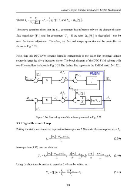
The above equations show that the
U
sx
component has influence only on the change of stator
flux magnitude
Ψ
s
, and the component
Ω
U
sy
– if the term
Ψs s
Ψ is decoupled – can be
used for torque adjustment. Therefore, the flux and torque quantities can be controlled as
shown in Fig. 5.26.
Note, that this DTC-SVM scheme formally corresponds to the stator flux oriented voltage
source inverter-fed drive induction motor. The block diagram of the DTC-SVM scheme with
two PI controllers is shown in Fig. 5.26 The dashed line represents the PMSM part [124,125].
Ψ s _ ref
Ψ s
_
R I
s
sx
U sx
R I
s
sx
∫
Ψ s
R I
s
sy
Ω Ψs
⊗
Ω
Ψ
Ψs s
M e _ ref
_
E sy
U sy
1 Isy
R s
3
2
p
b
Ψ
s _ ref
M e
M e
5.3.1 Digital flux control loop
Figure 5.26. Block diagram of the scheme presented in Fig. 5.27
Putting the stator x-axis current expression from equation 2.28a under the assumption Ld
= L
q
into equation (5.37) one can obtaines
U
I
sx
Ψs
−ΨPM
cos
= (5.39)
L
s
δ Ψ
Ψs −ΨPM cosδΨ
d Ψs R d Ψ
s s RsΨ
PM
= R ( ) + = Ψ + − cosδΨ
(5.40)
L dt L dt L
sx s s
s s s
Using Laplace transformation to equation 5.40 can be written as:
U
sx
Rs RsΨ
PM
=Ψ
s
( s+ ) − cosδ Ψ
. (5.41)
L L
s
s
89