Direct Torque Control with Space Vector Modulation (DTC-SVM) of ...

Direct Torque Control with Space Vector Modulation
PI controller
Time delay
G ( ) M
z
Dz ( )} Plant
M
e_ ref( z)
C ( ) M
z
U sy
z −1
AM
s
ZOH
2
s + B s+
C
M
M
M ( ) e
z
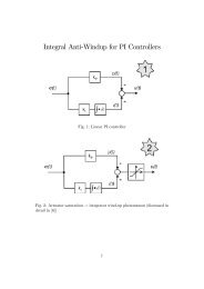
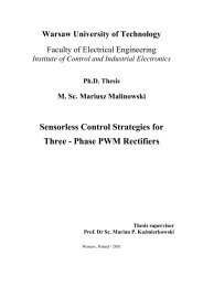
Figure 5.36. Block diagram of torque control loop in discrete domain.
Where: CM
( z)
- discrete transfer function for PI controller, Dz ( )
delay for voltage generation from PWM block (see Fig. 5.36).
1
z − - one sampling time
The discrete transfer function G ( z ) for voltage-torque relationship with zero order hold
(ZOH) can be calculated as:
M
G () s z −1
A
G z z Z Z
−1
M
M
M
( ) = (1 − ) [ ] = [ ]
2
s z s + BMs+
CM
⎡
⎤
⎡ ⎤ ⎢ ⎥
⎢ ⎥
z−1 AM
z−1
⎢ A
⎥
M
= Z ⎢
⎥ = Z
2
⎢
2
2
⎥ =
z ⎢⎛ B 2
M ⎞ B ⎥ z
M ⎢ B ⎛
M 2 B ⎞ ⎥
⎢⎜s+ ⎟ + CM
− ⎥
M
2 4 ⎢( s+ ) + CM
−
⎥
⎣⎝ ⎠ ⎦
⎢ 2 ⎜ 4 ⎟
⎣ ⎝ ⎠ ⎥⎦
.
⎡
⎤
2
⎢
B ⎥
M
CM
−
z −1 A ⎢
M
Z
4
⎥
= ⎢
2
2
⎥
z B 2
M
⎢
C B ⎛
M 2 B ⎞ ⎥
M
M
−
4
⎢( s+ ) + CM
−
⎥
⎢ 2 ⎜ 4 ⎟
⎣ ⎝ ⎠ ⎥⎦
(5.76)
Assuming that
have:
B
a = M
and
2
2
BM
b= CM
− , and using table of Z transformation [2] we
4
−aTs
⎡ b ⎤ ze sin( bTs
)
Z ⎢ 2 2 2 aTs
( s a) b
⎥ =
−
⎣ + + ⎦ z − 2 e (cos( bTs
)) z+
e
−2aTs
(5.77)
102