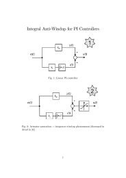
Linear Matrix Inequalities in Control
Linear Matrix Inequalities in Control
Linear Matrix Inequalities in Control

You also want an ePaper? Increase the reach of your titles
YUMPU automatically turns print PDFs into web optimized ePapers that Google loves.
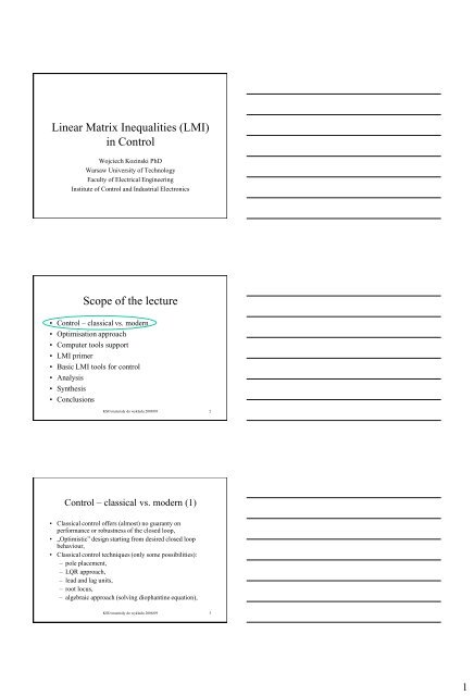
<strong>L<strong>in</strong>ear</strong> <strong>Matrix</strong> <strong>Inequalities</strong> (LMI)<br />
<strong>in</strong> <strong>Control</strong><br />
Wojciech Koz<strong>in</strong>ski PhD<br />
Warsaw University of Technology<br />
Faculty of Electrical Eng<strong>in</strong>eer<strong>in</strong>g<br />
Institute of <strong>Control</strong> and Industrial Electronics<br />
Scope of the lecture<br />
• <strong>Control</strong> – classical vs. modern<br />
• Optimisation approach<br />
• Computer tools support<br />
• LMI primer<br />
• Basic LMI tools for control<br />
• Analysis<br />
• Synthesis<br />
• Conclusions<br />
KSO materiały do wykładu 2008/09 2<br />
<strong>Control</strong> – classical vs. modern (1)<br />
• Classical control offers (almost) no guaranty on<br />
performance or robustness of the closed loop,<br />
• „Optimistic” design start<strong>in</strong>g from desired closed loop<br />
behaviour,<br />
• Classical control techniques (only some possibilities):<br />
– pole placement,<br />
– LQR approach,<br />
– lead and lag units,<br />
– root locus,<br />
– algebraic approach (solv<strong>in</strong>g diophant<strong>in</strong>e equation),<br />
KSO materiały do wykładu 2008/09 3<br />
1
<strong>Control</strong> – classical vs. modern (2)<br />
• Modern control techniques,<br />
– H analysis and synthesis,<br />
– H 2<br />
analysis and synthesis,<br />
– mixed criteria (+ pole placement),<br />
• They offer upper bounds estimates on performance and<br />
robustness of the closed loop,<br />
• They can tackle difficult problems,<br />
• Some disadvantages (high order controllers, a lot of<br />
mathematics, unable to solve some important problems).<br />
KSO materiały do wykładu 2008/09 4<br />
Scope of the lecture<br />
• <strong>Control</strong> – classical vs. modern<br />
• Optimisation approach<br />
• Computer tools support<br />
• LMI primer<br />
• Basic LMI tools for control<br />
• Analysis<br />
• Synthesis<br />
• Conclusions<br />
KSO materiały do wykładu 2008/09 5<br />
Optimisation approach (general)<br />
w<br />
p<br />
u<br />
Δ<br />
P<br />
K<br />
q<br />
y<br />
z<br />
x<br />
q<br />
y<br />
z<br />
u<br />
p<br />
Ax B1<br />
p B2w<br />
B3u<br />
C x D p D w D u<br />
q<br />
C x<br />
y<br />
Czx<br />
K y<br />
q<br />
D<br />
D<br />
q1<br />
y1<br />
z1<br />
p<br />
p<br />
q2<br />
D<br />
y2<br />
w<br />
D w D u<br />
z2<br />
q3<br />
z3<br />
f<strong>in</strong>d<br />
m<strong>in</strong><br />
K<br />
T<br />
zw p<br />
forall<br />
KSO materiały do wykładu 2008/09 6<br />
2
Optimisation approach (2)<br />
scalar signal norms<br />
L<br />
L 2<br />
norm - amplitude<br />
f ( t)<br />
sup f ( t)<br />
f<br />
t 0<br />
norm - energy<br />
1<br />
( d<br />
2<br />
2<br />
2<br />
f t)<br />
dt fˆ(<br />
)<br />
2<br />
0<br />
2<br />
KSO materiały do wykładu 2008/09 7<br />
Optimisation approach (3)<br />
system norm H<br />
System description (causal, with L 2 ga<strong>in</strong> γ>=0)<br />
x ( t)<br />
Ax(<br />
t)<br />
Bf ( t)<br />
y(<br />
t)<br />
Cx(<br />
t)<br />
Df ( t)<br />
H(<br />
s)<br />
C(<br />
sI<br />
Norm def<strong>in</strong>ition L 2 ga<strong>in</strong><br />
T<br />
T<br />
2<br />
2<br />
y(<br />
t)<br />
dt<br />
c<br />
0<br />
0<br />
H sup H(<br />
j<br />
R<br />
2<br />
f ( t)<br />
dt<br />
Norm <strong>in</strong>terpretation<br />
) H<br />
sup max<br />
R<br />
( H(<br />
j<br />
A)<br />
))<br />
1<br />
B<br />
D<br />
KSO materiały do wykładu 2008/09 8<br />
Optimisation approach (4)<br />
system norm H calculations<br />
Theorem<br />
Let A be a Hurwitz (stable) matrix. Then the L 2 ga<strong>in</strong> of the<br />
system is less than γ if and only if max(<br />
D)<br />
and the matrix<br />
F<br />
2<br />
A B(<br />
I<br />
T T<br />
C C C D(<br />
T 1 T<br />
D D)<br />
D C<br />
2 T 1 T<br />
I D D)<br />
D C<br />
2 T 1 T<br />
B(<br />
I D D)<br />
B<br />
T T 2 T<br />
A C D(<br />
I D D)<br />
1<br />
B<br />
does not have eigenvalues on the imag<strong>in</strong>ary axis.<br />
H<strong>in</strong>t : use bisection method.<br />
KSO materiały do wykładu 2008/09 9<br />
3
H<br />
2<br />
2<br />
Optimisation approach (5)<br />
– norm H 2<br />
If the <strong>in</strong>put <strong>in</strong>to system is white noise then output<br />
variance is called H 2 norm<br />
lim E y(<br />
t)<br />
t<br />
0<br />
2<br />
H<br />
If h(t) is impulse response matrix of the system, then<br />
T<br />
trace(<br />
h(<br />
t)<br />
h(<br />
t))<br />
dt<br />
2<br />
2<br />
1<br />
2<br />
T<br />
trace(<br />
H(<br />
j ) H(<br />
j )) d<br />
KSO materiały do wykładu 2008/09 10<br />
Optimisation approach (6)<br />
system norm calculations<br />
H 2<br />
Theorem:<br />
Let A be a Hurwitz matrix. The H 2 norm of the system is<br />
<strong>in</strong>f<strong>in</strong>ite if D 0.<br />
Otherwise, it equals:<br />
2<br />
T<br />
( ) trace T<br />
H trace CPC ( B QB)<br />
2<br />
Where P=P T and Q=Q T are the unique solutions of the<br />
Lapunov equations:<br />
AP<br />
T<br />
PA<br />
BB<br />
T<br />
T<br />
T<br />
0;<br />
A Q QA C C<br />
0<br />
KSO materiały do wykładu 2008/09 11<br />
Optimisation approach (7)<br />
<strong>L<strong>in</strong>ear</strong> Fractional Transformation (LFT)<br />
z1<br />
y1<br />
M<br />
l<br />
w1<br />
u1<br />
z1<br />
y<br />
u<br />
T<br />
1<br />
1<br />
zw1<br />
w1<br />
M<br />
u<br />
l<br />
y<br />
F<br />
1<br />
M<br />
M<br />
11<br />
21<br />
M<br />
M<br />
12<br />
22<br />
w1<br />
u<br />
1<br />
1<br />
l<br />
( M,<br />
l<br />
) M11<br />
M12<br />
l<br />
( I M22<br />
l<br />
) M21<br />
1<br />
z2<br />
y2<br />
u<br />
M<br />
u2<br />
w 2<br />
z2<br />
y<br />
u<br />
T<br />
2<br />
2<br />
zw2<br />
w2<br />
M<br />
u<br />
u<br />
F<br />
y<br />
2<br />
M<br />
M<br />
11<br />
21<br />
M<br />
M<br />
12<br />
22<br />
w2<br />
u<br />
2<br />
1<br />
u( M,<br />
u)<br />
M22<br />
M21<br />
u(<br />
I M11<br />
u)<br />
M12<br />
2<br />
KSO materiały do wykładu 2008/09 12<br />
4
Optimisation approach (8)<br />
Analysis - example<br />
w<br />
u<br />
e<br />
F C Go<br />
q<br />
Δ<br />
+<br />
p<br />
z<br />
-<br />
G<br />
0<br />
1<br />
; C<br />
2<br />
s<br />
F<strong>in</strong>d the largest<br />
2.35(1 s)<br />
;<br />
(1 0.1s<br />
)<br />
F<br />
1.2<br />
;<br />
s 1.2<br />
and ma<strong>in</strong>ta<strong>in</strong> stability<br />
KSO materiały do wykładu 2008/09 13<br />
Optimisation approach (9)<br />
Synthesis - example<br />
w<br />
-<br />
1<br />
s<br />
-<br />
10<br />
z<br />
Gi(s) G i<br />
( s)<br />
;<br />
2<br />
s as b<br />
x<br />
K a 1..3 ; b 8..12 ;<br />
For all plants G i (s) f<strong>in</strong>d stabilis<strong>in</strong>g<br />
static state space controller K.<br />
KSO materiały do wykładu 2008/09 14<br />
Optimisation approach (10)<br />
when the synthesis is well-posed?<br />
w<br />
u<br />
P(s)<br />
K(s)<br />
Closed loop description:<br />
cl<br />
y<br />
z<br />
x<br />
Ax B1w<br />
B2u<br />
z C1x<br />
D11w<br />
D12u<br />
y C x D w D u<br />
x f<br />
u<br />
2<br />
A x<br />
C x<br />
f<br />
f<br />
KSO materiały do wykładu 2008/09 15<br />
f<br />
f<br />
21<br />
D y<br />
22<br />
B y<br />
x A x B w x<br />
cl cl cl<br />
xcl<br />
z Cclxcl<br />
Dclw<br />
x<br />
f<br />
M<strong>in</strong>imize some measure ( T ) ( F ( P,<br />
K))<br />
w z<br />
l<br />
f<br />
f<br />
5
Optimisation approach (11)<br />
when the synthesis is well-posed?<br />
A<br />
C<br />
cl<br />
cl<br />
A B2D f<br />
C2<br />
B C<br />
C<br />
1<br />
f<br />
12<br />
2<br />
D D C<br />
f<br />
2<br />
B2C<br />
f<br />
A<br />
f<br />
D C ; D<br />
12<br />
; B<br />
f<br />
cl<br />
cl<br />
B1<br />
Df<br />
D<br />
B D<br />
D<br />
11<br />
f<br />
21<br />
12<br />
21<br />
D D D<br />
1. Simultanouos stabilisability of the pair (A,B 2 ) and observability of the pair<br />
(C 2 ,A).<br />
2. D-matrix conditions:<br />
1. D 22 =0,<br />
2. D cl =0 (if H 2 norm is used),<br />
3. often D 11 =0 required (Robust Toolbox),<br />
4. D 12 full column rank matrix,<br />
5. D 21 full row rank matrix.<br />
f<br />
21<br />
KSO materiały do wykładu 2008/09 16<br />
Optimisation approach (warn<strong>in</strong>g)<br />
• Many (all ?) control analysis and synthesis problems can be formulated<br />
as optimisation problems.<br />
• Only some of them can be transformed <strong>in</strong>to LMI (not BMI), solvable<br />
problems (e.g. there exists no general output controller synthesis for<br />
uncerta<strong>in</strong> plant – like LFT framework).<br />
• As LMI – the price is paid <strong>in</strong> large number of slack (Lapunov)<br />
variables.<br />
• Many <strong>in</strong>terest<strong>in</strong>g papers on BMI solvers and non-smooth, non-convex<br />
optimisation have been published recently. P.Apkarian ONERA-CERT,<br />
D. Noll Uni Toulouse, M.Overton, Uni of New York.<br />
KSO materiały do wykładu 2008/09 17<br />
Scope of the lecture<br />
• <strong>Control</strong> – classical vs. modern<br />
• Optimisation approach<br />
• Computer tools support<br />
• LMI primer<br />
• Basic LMI tools for control<br />
• Analysis<br />
• Synthesis<br />
• Conclusions<br />
KSO materiały do wykładu 2008/09 18<br />
6
Computer tools support<br />
• Matlab ® Robust <strong>Control</strong> Toolbox<br />
• Public doma<strong>in</strong> SDP-solvers (Matlab ® based):<br />
– SP (Boyd & Vanderberghe) –old,<br />
– SeDuMi (Sturm, now – McMaster University),<br />
• Public doma<strong>in</strong> preprocessors<br />
– YALMIP (Löfberg <strong>in</strong> ETH Zurich):<br />
• Many other possibilities (see YALMIP www<br />
page)<br />
KSO materiały do wykładu 2008/09 19<br />
Scope of the lecture<br />
• <strong>Control</strong> – classical vs. modern<br />
• Optimisation approach<br />
• Computer tools support<br />
• LMI primer<br />
• Basic LMI tools for control<br />
• Analysis<br />
• Synthesis<br />
• Conclusions<br />
KSO materiały do wykładu 2008/09 20<br />
F(<br />
x)<br />
LMI Primer (1) - def<strong>in</strong>ition<br />
LMI is a matrix dependent on vector x<br />
F<br />
0<br />
m<br />
i 1<br />
T<br />
z Fz<br />
x i<br />
F i<br />
0,<br />
z<br />
0<br />
where m<br />
x R , Fi<br />
Positive def<strong>in</strong>ite matrix F is such that<br />
0, z<br />
n<br />
R .<br />
n n<br />
If LMI has a solution (is feasible) then the solution is a<br />
non empty set. The solution set is convex.<br />
x|<br />
F(<br />
x)<br />
0<br />
KSO materiały do wykładu 2008/09 21<br />
R<br />
7
LMI Primer (2)<br />
There are many LMIs which have the same solution:<br />
Let M R<br />
n n<br />
; det( M)<br />
0 and x M z<br />
then by congruence can be obta<strong>in</strong>ed:<br />
T<br />
T T<br />
T<br />
A 0 x Ax 0 z M AMz 0 M AM<br />
An example:<br />
A B<br />
0<br />
C D<br />
0 I A B<br />
I 0 C D<br />
0 I<br />
0<br />
I 0<br />
D C<br />
0<br />
B A<br />
0<br />
KSO materiały do wykładu 2008/09 22<br />
LMI Primer (3)<br />
Multiple LMIs can be expressed as a s<strong>in</strong>gle LMI.<br />
Set def<strong>in</strong>ed by by q LMIs:<br />
F(<br />
x)<br />
1<br />
F ( x)<br />
2<br />
0; F ( x)<br />
An equivalent s<strong>in</strong>gle LMI:<br />
where<br />
q<br />
0;...; F ( x)<br />
m<br />
0<br />
xiFi<br />
x<br />
i 1<br />
F<br />
1 2<br />
q<br />
diag F ( x)<br />
F ( x)<br />
... F ( ) 0<br />
1 2<br />
q<br />
Fi diagFi<br />
Fi<br />
... Fi<br />
; i 0,1 ,..., m<br />
0<br />
KSO materiały do wykładu 2008/09 23<br />
LMI Primer (4)<br />
<strong>L<strong>in</strong>ear</strong> constra<strong>in</strong>ts can be expressed as an LMI:<br />
General l<strong>in</strong>ear constra<strong>in</strong>t:<br />
Ax<br />
b<br />
where<br />
n<br />
b R ,<br />
A<br />
R<br />
,<br />
n m<br />
x<br />
m<br />
R .<br />
can be converted to n scalar <strong>in</strong>equalities <strong>in</strong> LMI form<br />
m<br />
bi Aijx<br />
j<br />
0; i 1,...,<br />
n<br />
j 1<br />
and then <strong>in</strong>to s<strong>in</strong>gle LMI.<br />
KSO materiały do wykładu 2008/09 24<br />
8
LMI Primer (5)<br />
The Schur complement lemma:<br />
Converts convex nonl<strong>in</strong>ear <strong>in</strong>equality<br />
R(<br />
x)<br />
where<br />
0,<br />
Q(<br />
x)<br />
1 T<br />
S(<br />
x)<br />
R(<br />
x)<br />
S(<br />
x)<br />
T<br />
T<br />
Q( x)<br />
Q(<br />
x)<br />
, R(<br />
x)<br />
R(<br />
x)<br />
0 and S(<br />
x)<br />
<strong>in</strong>to the equivalent LMI<br />
Q(<br />
x)<br />
T<br />
S(<br />
x)<br />
S(<br />
x)<br />
R(<br />
x)<br />
Very important lemma!<br />
0<br />
0<br />
depend aff<strong>in</strong>ely on x<br />
KSO materiały do wykładu 2008/09 25<br />
The condition<br />
( A(<br />
x))<br />
1<br />
I<br />
A(<br />
x)<br />
T<br />
LMI Primer (6)<br />
Maximum s<strong>in</strong>gular value: is def<strong>in</strong>ed as:<br />
T<br />
( A(<br />
x))<br />
max(<br />
A(<br />
x)<br />
A(<br />
x)<br />
)<br />
where matrix A(x) depends aff<strong>in</strong>ely on x<br />
( A(<br />
x))<br />
1 can be expressed as a LMI<br />
A(<br />
x)<br />
A(<br />
x)<br />
A(<br />
x)<br />
0<br />
I<br />
T<br />
I I<br />
A(<br />
x)<br />
A(<br />
x)<br />
T<br />
0<br />
KSO materiały do wykładu 2008/09 26<br />
whereP<br />
LMI Primer (7)<br />
Algebraic Riccati <strong>in</strong>equality:<br />
T<br />
1 T<br />
A P PA PBR B P Q 0<br />
P<br />
T<br />
T<br />
0; Q Q ; R 0;<br />
can be expressed as a LMI<br />
T<br />
A P PA<br />
T<br />
B P<br />
Q<br />
PB<br />
R<br />
0;<br />
P<br />
0.<br />
KSO materiały do wykładu 2008/09 27<br />
9
LMI Primer (8)<br />
• Three types of LMI problems<br />
– feasibility problem LMIP,<br />
A(x) 0<br />
– eigenvalue problem EVP,<br />
m<strong>in</strong>imum c T x subject to A(x) 0<br />
– generalised eigenvalue problem GEVP,<br />
m<strong>in</strong>imum λ subject to A( x)<br />
B(<br />
x);<br />
B(<br />
x)<br />
0; C(<br />
x)<br />
where<br />
T<br />
T<br />
B ( x)<br />
B(<br />
x)<br />
0; A(<br />
x)<br />
A(<br />
x)<br />
0.<br />
KSO materiały do wykładu 2008/09 28<br />
Scope of the lecture<br />
• <strong>Control</strong> – classical vs. modern<br />
• Optimisation approach<br />
• Computer tools support<br />
• LMI primer<br />
• Basic LMI tools for control<br />
• Analysis<br />
• Synthesis<br />
• Conclusions<br />
KSO materiały do wykładu 2008/09 29<br />
Basic LMI tools for control (1)<br />
Stability<br />
Autonomous l<strong>in</strong>ear system<br />
x<br />
Ax<br />
T<br />
Lapunov function V( x)<br />
x Px 0 except x<br />
Condition on it’s derivative:<br />
dV(<br />
x)<br />
dt<br />
x Px<br />
T<br />
x Px<br />
T T<br />
x ( A P<br />
LMI for stability A T P PA<br />
0<br />
PA)<br />
x<br />
0<br />
P<br />
0<br />
T<br />
A P<br />
0<br />
PA<br />
0<br />
KSO materiały do wykładu 2008/09 30<br />
10
Basic LMI tools for control (2)<br />
Stability<br />
Equivalence between LMI def<strong>in</strong>ition and matrix formula<br />
p1<br />
p2<br />
Example for n=2 P<br />
0<br />
p p<br />
A T P PA<br />
2a<br />
p1<br />
a<br />
11<br />
12<br />
a12<br />
0<br />
a<br />
a<br />
11<br />
12<br />
a<br />
a<br />
21<br />
22<br />
11<br />
p1<br />
p<br />
2<br />
2<br />
2a21<br />
p2<br />
a a<br />
22<br />
p2<br />
p<br />
3<br />
3<br />
a11<br />
a<br />
2a<br />
12<br />
p1<br />
p<br />
2<br />
22<br />
p2<br />
p<br />
3<br />
a<br />
a<br />
11<br />
21<br />
0<br />
p3<br />
a<br />
21<br />
a<br />
a<br />
12<br />
22<br />
a<br />
2a<br />
21<br />
22<br />
KSO materiały do wykładu 2008/09 31<br />
Basic LMI tools for control (3)<br />
Stability<br />
Additional conditions on s-plane regions<br />
Guaranteed damp<strong>in</strong>g<br />
C stab<br />
{ s C | re(<br />
s)<br />
} s s 2 0<br />
Maximal damp<strong>in</strong>g and oscillation<br />
r s q<br />
C stab<br />
{ s C | s q r}<br />
0<br />
s q r<br />
Vertical strip<br />
( s s)<br />
2<br />
2<br />
0<br />
C stab<br />
{ s C |<br />
1<br />
re(<br />
s)<br />
2}<br />
0<br />
0 ( s s)<br />
2<br />
1<br />
KSO materiały do wykładu 2008/09 32<br />
Basic LMI tools for control (4)<br />
Stability<br />
Theorem:<br />
All eigenvalues of the real matrix A are <strong>in</strong> the region<br />
described by C<br />
stab<br />
{ s C|<br />
P Qs<br />
T<br />
Q s 0}<br />
with P<br />
T<br />
P<br />
if and only if there exists symmetric matrix X=X T >0<br />
p X<br />
p<br />
11<br />
k1<br />
X<br />
q11AX<br />
<br />
q AX<br />
k1<br />
T<br />
q11XA<br />
<br />
<br />
T<br />
q XA<br />
1k<br />
T<br />
p1<br />
k<br />
X q1<br />
k<br />
AX qk1XA<br />
<br />
T<br />
p X q AX q XA<br />
kk<br />
kk<br />
kk<br />
0<br />
Equivalent LMI us<strong>in</strong>g Kronecker multiplication:<br />
P X Q AX<br />
Q<br />
T<br />
XA<br />
T<br />
0<br />
KSO materiały do wykładu 2008/09 33<br />
11
Basic LMI tools for control (6)<br />
Stability – example - feasibility<br />
For given real matrix A check<br />
it its eigenvalues are <strong>in</strong>side<br />
the selected region:<br />
• usage of previously presented<br />
theorem,<br />
• feasibility type problem,<br />
r<br />
-4 -2<br />
q=-3<br />
Im<br />
1<br />
Re<br />
0<br />
-1<br />
KSO materiały do wykładu 2008/09 34<br />
Optimiser: SeDuMi<br />
Demo no.1<br />
Preprocesor: YALMIP<br />
Given is matrix A with eigenvalues -1 j1. If radius of the<br />
circle with orig<strong>in</strong> (-3,0) is greater then sqrt(5) the problem<br />
is feasible, otherwise unfeasible.<br />
KSO materiały do wykładu 2008/09 35<br />
Basic LMI tools for control (7)<br />
Stability of non-l<strong>in</strong>ear/time-vary<strong>in</strong>g<br />
Two admissible descriptions of autonomous non-l<strong>in</strong>ear<br />
or time vary<strong>in</strong>g system <strong>in</strong> form of convex hull of matrices:<br />
x t)<br />
A(<br />
t)<br />
x(<br />
t),<br />
A(<br />
t)<br />
Co{<br />
A,<br />
A ,... A }<br />
(<br />
1 2 L<br />
L<br />
x ( t)<br />
A(<br />
t)<br />
x(<br />
t),<br />
A(<br />
t)<br />
LMIs to prove stability:<br />
i<br />
A i<br />
i 1<br />
T<br />
P P 0<br />
T<br />
Ai P PAi<br />
0, i 1,...,<br />
L<br />
,<br />
i<br />
0,<br />
L<br />
i<br />
i 1<br />
1.<br />
KSO materiały do wykładu 2008/09 36<br />
12
Basic LMI tools for control (8)<br />
Bounded real lemma<br />
The system def<strong>in</strong>ition<br />
x Ax Bu<br />
G(<br />
s)<br />
sup ( G(<br />
s))<br />
sup ( G(<br />
j ))<br />
Re( s)<br />
0<br />
R<br />
y Cx Du<br />
x(0)<br />
0<br />
G(<br />
s)<br />
1<br />
C(<br />
sI A)<br />
B<br />
M<strong>in</strong>imize γ 2 subject to:<br />
T<br />
T<br />
T<br />
A P PA C C PB C D<br />
T T<br />
T 2<br />
B P D C D D I<br />
D<br />
F<strong>in</strong>d (the upper bound)<br />
0; P<br />
P<br />
T<br />
0<br />
KSO materiały do wykładu 2008/09 37<br />
Basic LMI tools for control (9)<br />
S-procedure (simplified)<br />
If there exist symmetric matrices T 0 ,...,T p and nonnegative<br />
numbers<br />
1<br />
0,...,<br />
p<br />
0 such that<br />
T<br />
0<br />
i<br />
p<br />
1<br />
iT i<br />
0<br />
T<br />
T<br />
then x T0 x 0; x 0if<br />
x Ti<br />
x 0; i 1, ,<br />
p.<br />
For p=1 the reverse is true.<br />
KSO materiały do wykładu 2008/09 38<br />
Basic LMI tools for control (10)<br />
S-procedure example<br />
There are two condtions given for P<br />
P<br />
T<br />
0,<br />
0 and any<br />
T<br />
T<br />
A P PA<br />
T<br />
B P<br />
PB<br />
0<br />
0<br />
T C T C<br />
T<br />
A P<br />
PA<br />
T<br />
B P<br />
T<br />
C C<br />
PB<br />
I<br />
0; P<br />
P<br />
T<br />
T .<br />
Us<strong>in</strong>g S-procedure one can obta<strong>in</strong> LMIs:<br />
0;<br />
0<br />
KSO materiały do wykładu 2008/09 39<br />
13
Basic LMI tools for control (11)<br />
H <strong>in</strong>f norm calculations<br />
For system:<br />
x<br />
y<br />
Ax<br />
Cx<br />
M<strong>in</strong>imize γ subject to:<br />
T<br />
A X XA<br />
T<br />
B X<br />
C<br />
XB<br />
I<br />
D<br />
T<br />
C<br />
T<br />
D<br />
I<br />
Bu<br />
Du<br />
0; X<br />
Variable γ is the upper bound of H <strong>in</strong>f<br />
0; whereX<br />
T<br />
X .<br />
KSO materiały do wykładu 2008/09 40<br />
Optimiser: SeDuMi<br />
Let<br />
G( s)<br />
2<br />
s<br />
10<br />
2s<br />
10<br />
Demo no.2<br />
The state space representation is<br />
A<br />
2<br />
8<br />
1.25<br />
; B<br />
0<br />
Preprocesor: YALMIP<br />
1<br />
; C<br />
0<br />
0 1.25; D 0.<br />
F<strong>in</strong>d norm H <strong>in</strong>f and compare it with the result of Matlab ®<br />
function.<br />
KSO materiały do wykładu 2008/09 41<br />
Basic LMI tools for control (12)<br />
H 2 norm calculations<br />
For system:<br />
x<br />
y<br />
Ax<br />
Cx<br />
Bu<br />
M<strong>in</strong>imize trace(Q) subject to:<br />
T T<br />
AP PA BB 0<br />
Q<br />
PC<br />
T<br />
whereP<br />
CP<br />
P<br />
T<br />
P , Q<br />
0; P<br />
0<br />
T<br />
Q .<br />
KSO materiały do wykładu 2008/09 42<br />
14
Optimiser: SeDuMi<br />
Demo no.3<br />
Preprocesor: YALMIP<br />
Let<br />
G( s)<br />
2<br />
s<br />
10<br />
2s<br />
10<br />
The state space representation is<br />
A<br />
2<br />
8<br />
1.25<br />
; B<br />
0<br />
1<br />
; C<br />
0<br />
0<br />
1.25; D<br />
0.<br />
F<strong>in</strong>d norm H 2 and compare it with the result of Matlab ®<br />
function.<br />
KSO materiały do wykładu 2008/09 43<br />
Scope of the lecture<br />
• <strong>Control</strong> – classical vs. modern<br />
• Optimisation approach<br />
• Computer tools support<br />
• LMI primer<br />
• Basic LMI tools for control<br />
• Analysis<br />
• Synthesis<br />
• Conclusions<br />
KSO materiały do wykładu 2008/09 44<br />
Analysis (1)<br />
Robustness problems<br />
1. Robust stability,<br />
2. Robust performance.<br />
Question: what is the biggest admissible Δ ?<br />
G G G 0<br />
( I )<br />
G 0<br />
Δ<br />
Δ<br />
G0<br />
G0<br />
KSO materiały do wykładu 2008/09 45<br />
15
Analysis (2)<br />
Uncerta<strong>in</strong>ity descriptions<br />
1. Norm-bounded uncerta<strong>in</strong>ity without structure<br />
1<br />
( s)<br />
W(<br />
s)<br />
2. Norm-bounded uncerta<strong>in</strong>ity with structure<br />
Δ partitioned <strong>in</strong>to blocks with their own bounds<br />
3. Sector-bounded uncerta<strong>in</strong>ity (dynamic or static)<br />
mapp<strong>in</strong>g : u L y L<br />
0<br />
( y(<br />
t)<br />
2<br />
T<br />
au(<br />
t))<br />
( y(<br />
t)<br />
2<br />
bu(<br />
t))<br />
dt<br />
1<br />
0<br />
KSO materiały do wykładu 2008/09 46<br />
Analysis (3)<br />
Robust stability – problem statement<br />
w<br />
p<br />
Δ<br />
P<br />
q<br />
z<br />
x<br />
q<br />
z<br />
p<br />
Ax B1<br />
p B2w<br />
C1x<br />
D11p<br />
D12w<br />
C2x<br />
D21p<br />
D22w<br />
q<br />
1<br />
Is the system stable for all admissible Δ?<br />
KSO materiały do wykładu 2008/09 47<br />
M<br />
1<br />
Analysis (3)<br />
Robust stability – LMIs<br />
T<br />
A P PA<br />
T<br />
B P<br />
PB<br />
0<br />
B<br />
B 1<br />
B 2<br />
M<br />
2<br />
C2<br />
0<br />
D<br />
0<br />
21<br />
T<br />
22<br />
D<br />
I<br />
I<br />
0<br />
0<br />
2<br />
I<br />
C2<br />
0<br />
D<br />
0<br />
21<br />
D<br />
I<br />
22<br />
M<br />
3<br />
C1<br />
D<br />
0 I<br />
11<br />
T<br />
D12<br />
I 0<br />
0 0 I<br />
C1<br />
D11<br />
D<br />
0 I 0<br />
m<strong>in</strong> s.<br />
t.(<br />
M1 M2<br />
M3<br />
0; P 0;<br />
12<br />
0)<br />
KSO materiały do wykładu 2008/09 48<br />
16
Analysis (4)<br />
Robust stability – example<br />
q Δ<br />
k<br />
w<br />
u<br />
e<br />
F C G o<br />
k<br />
p<br />
z<br />
2<br />
k<br />
q<br />
z<br />
2<br />
k G0C(<br />
I G0C)<br />
1<br />
k(<br />
I G C)<br />
0<br />
1<br />
kG0CF(<br />
I<br />
G CF(<br />
I<br />
0<br />
G0C)<br />
G C)<br />
0<br />
1<br />
1<br />
p<br />
w<br />
KSO materiały do wykładu 2008/09 49<br />
A<br />
C<br />
A<br />
Analysis (5)<br />
Robust stability – example<br />
G<br />
0<br />
C1<br />
C<br />
k max<br />
2<br />
0<br />
1<br />
; C<br />
2<br />
s<br />
B0Dr<br />
C<br />
BrC0<br />
0<br />
kC0<br />
C<br />
0<br />
0<br />
0.748<br />
B0Cr<br />
Ar<br />
0<br />
2.35(1 s)<br />
; F<br />
(1 0.1s<br />
)<br />
0 0<br />
; D<br />
0 0<br />
B0Dr<br />
C<br />
f<br />
BrC<br />
f<br />
A<br />
f<br />
D<br />
D<br />
11<br />
21<br />
; B<br />
D<br />
D<br />
12<br />
22<br />
1.2<br />
;<br />
s 1.2<br />
B0Dr<br />
k<br />
Brk<br />
0<br />
0<br />
k<br />
0<br />
0<br />
KSO materiały do wykładu 2008/09 50<br />
;<br />
B0Dr<br />
Df<br />
Br<br />
Df<br />
B<br />
f<br />
;<br />
Demo no.4<br />
Optimiser: SeDuMi<br />
Preprocesor: YALMIP<br />
Run the presented example with some simulations to<br />
confirm the result.<br />
KSO materiały do wykładu 2008/09 51<br />
17
Analysis (6)<br />
Integral Quadratic Constra<strong>in</strong>ts (IQC)<br />
Powerful method for <strong>in</strong>vestigat<strong>in</strong>g stability of uncerta<strong>in</strong> systems<br />
.<br />
Let pˆ and qˆ<br />
be Fourier Transforms of p and q signals.<br />
.<br />
IQC is def<strong>in</strong>ed by ( j ) where<br />
pˆ(<br />
j<br />
qˆ(<br />
j<br />
)<br />
)<br />
*<br />
( j<br />
pˆ(<br />
j<br />
)<br />
qˆ(<br />
j<br />
)<br />
d<br />
)<br />
0<br />
KSO materiały do wykładu 2008/09 52<br />
Analysis (7)<br />
Integral Quadratic Constra<strong>in</strong>ts (IQC)<br />
For autonomous system<br />
x<br />
( t)<br />
Ax(<br />
t)<br />
B p(<br />
t)<br />
q(<br />
t)<br />
p(<br />
t)<br />
C x(<br />
t)<br />
q<br />
q(<br />
t);<br />
p<br />
D p(<br />
t)<br />
qp<br />
01<br />
For small ε>0 it is true<br />
H(<br />
j )<br />
I<br />
*<br />
H(<br />
j )<br />
( j )<br />
I<br />
H(<br />
s)<br />
C ( sI<br />
1<br />
A)<br />
B<br />
KSO materiały do wykładu 2008/09 53<br />
q<br />
2 I for all<br />
Kalman-Yakubovich-Popov (KYP) lemma converts this<br />
condition <strong>in</strong>to LMI.<br />
R<br />
p<br />
D<br />
qp<br />
Analysis (8)<br />
Integral Quadratic Constra<strong>in</strong>ts (IQC)<br />
Kalman-Yakubovich-Popov (KYP) lemma:<br />
Let the pair of matrices (A,B) is stabilisable and matrix A has no<br />
eigenvalues on imag<strong>in</strong>ary axis. Then the statements are equivalent:<br />
( j<br />
1<br />
I A)<br />
B<br />
I<br />
T<br />
PA A P<br />
T<br />
B P<br />
*<br />
PB<br />
0<br />
( j<br />
1<br />
I A)<br />
B<br />
I<br />
0, P<br />
There is powerful Matlab ® toolbox called iqc-beta (from MIT).<br />
P<br />
T<br />
0,<br />
0<br />
0,<br />
KSO materiały do wykładu 2008/09 54<br />
18
Scope of the lecture<br />
• <strong>Control</strong> – classical vs. modern<br />
• Optimisation approach<br />
• Computer tools support<br />
• LMI primer<br />
• Basic LMI tools for control<br />
• Analysis<br />
• Synthesis<br />
• Conclusions<br />
KSO materiały do wykładu 2008/09 55<br />
Synthesis (1)<br />
What can be done with<strong>in</strong> LMI framework?<br />
• Design of static, state controller for uncerta<strong>in</strong><br />
plants with H 2 /H <strong>in</strong>f norm m<strong>in</strong>imization, pole<br />
placement,<br />
• Design of dynamic, output controller for nom<strong>in</strong>al<br />
plants with H 2 /H <strong>in</strong>f norm m<strong>in</strong>imization, pole<br />
placement,<br />
• Design of dynamic, output controller for uncerta<strong>in</strong><br />
plants with H 2 /H <strong>in</strong>f norm m<strong>in</strong>imization, pole<br />
placement, if uncerta<strong>in</strong>ity measurment is available<br />
(so called ga<strong>in</strong>-schedul<strong>in</strong>g).<br />
KSO materiały do wykładu 2008/09 56<br />
Synthesis (2)<br />
Typical strategy<br />
Pole placement and H <strong>in</strong>f +H 2 norms m<strong>in</strong>imisation,<br />
• Select the pole placement region and run the test to<br />
check, if it is feasible,<br />
• M<strong>in</strong>imise H <strong>in</strong>f norm to f<strong>in</strong>d the smallest possible one<br />
and controller,<br />
• For several, greater but fixed values of H <strong>in</strong>f norm<br />
m<strong>in</strong>imise H 2 norms,<br />
• Plot H 2 norms versus H <strong>in</strong>f fixed norms (Pareto like<br />
curve),<br />
• Select trade-off po<strong>in</strong>t or discard the design.<br />
KSO materiały do wykładu 2008/09 57<br />
19
Synthesis (3)<br />
Design of static, state controller<br />
w<br />
x<br />
z<br />
+<br />
u<br />
A x<br />
p<br />
C x<br />
p<br />
u Kx<br />
G<br />
K<br />
x<br />
B ( w<br />
p<br />
D ( w<br />
p<br />
z<br />
u)<br />
u)<br />
x<br />
z<br />
z<br />
z<br />
2<br />
w<br />
u<br />
KSO materiały do wykładu 2008/09 58<br />
P<br />
K<br />
x<br />
z2<br />
z<strong>in</strong>f<br />
z<br />
Ax Buu<br />
Bww<br />
C x D<br />
uu<br />
D<br />
ww<br />
C2x<br />
D2uu<br />
D2<br />
ww<br />
C x D u D w<br />
z<br />
zu<br />
zw<br />
2<br />
Synthesis (4)<br />
Design of static, state controller<br />
Norms def<strong>in</strong>itions (<strong>in</strong> signal terms)<br />
<strong>Matrix</strong> def<strong>in</strong>itions for general setup<br />
B<br />
C<br />
C<br />
C<br />
u<br />
z<br />
B ;<br />
p<br />
C ;<br />
Cp<br />
;<br />
0<br />
C ;<br />
p<br />
p<br />
B<br />
D<br />
w<br />
D<br />
D<br />
zu<br />
B ;<br />
u<br />
2u<br />
p<br />
D ;<br />
p<br />
D ;<br />
p<br />
Dp<br />
;<br />
1<br />
D<br />
zw<br />
D<br />
D<br />
w<br />
2w<br />
D ;<br />
p<br />
z w z;<br />
z2<br />
1 D ;<br />
p<br />
Dp<br />
;<br />
0<br />
z<br />
u<br />
KSO materiały do wykładu 2008/09 59<br />
Optimiser: SeDuMi<br />
G(<br />
s)<br />
1<br />
2<br />
s<br />
Demo no.5<br />
Preprocesor: YALMIP<br />
a) Pole placement and H <strong>in</strong>f m<strong>in</strong>imisation to obta<strong>in</strong> lower<br />
bound,<br />
b) Several runs – pole placement and H 2 m<strong>in</strong>imisation for<br />
fixed values H <strong>in</strong>f ,; generate Pareto-like curve,<br />
c) Pole placement and H <strong>in</strong>f + H 2 m<strong>in</strong>imisation.<br />
KSO materiały do wykładu 2008/09 60<br />
20
Synthesis (5)<br />
Design of static, state controller<br />
Analysis of the design (closed loop)<br />
x A x B w; x x; A A B K B B ;<br />
u<br />
z<br />
z<br />
z<br />
cl<br />
2<br />
cl<br />
cl<br />
cl<br />
K xcl;<br />
( C D<br />
uK)<br />
x<br />
( C2<br />
D2u<br />
K)<br />
xcl<br />
( C D K)<br />
x<br />
z<br />
zu<br />
cl<br />
If norm H 2 is used then<br />
cl<br />
cl<br />
D<br />
ww;<br />
D2<br />
ww;<br />
D w;<br />
D 2w<br />
zw<br />
0.<br />
cl<br />
;<br />
cl w<br />
KSO materiały do wykładu 2008/09 61<br />
u<br />
Synthesis (6)<br />
Design of static, state controller<br />
Another structure for uncerta<strong>in</strong> plants.<br />
w<br />
-<br />
e<br />
1/s<br />
v<br />
+<br />
u<br />
G<br />
K<br />
x<br />
z<br />
No problems with static ga<strong>in</strong>.<br />
KSO materiały do wykładu 2008/09 62<br />
Optimiser: SeDuMi<br />
Demo no.6<br />
10<br />
s)<br />
;<br />
s as b<br />
1..3 ; b 8..12 ;<br />
G i<br />
(<br />
2<br />
a<br />
Preprocesor: YALMIP<br />
Design state space controller for all „corner” plants<br />
us<strong>in</strong>g pole-placement.<br />
KSO materiały do wykładu 2008/09 63<br />
21
Synthesis (7)<br />
Design of dynamic, output controller<br />
w<br />
-<br />
u<br />
x Ax<br />
z Cx<br />
k<br />
x<br />
u<br />
Ak<br />
x<br />
C x<br />
k<br />
z<br />
G<br />
y<br />
Gk<br />
B(<br />
w u)<br />
D(<br />
w u)<br />
k<br />
k<br />
Bk<br />
y<br />
D y<br />
k<br />
w<br />
u<br />
P<br />
Gk<br />
z w z;<br />
z2<br />
y<br />
z<br />
u<br />
z2<br />
z<strong>in</strong>f<br />
z<br />
Design norms as an example<br />
KSO materiały do wykładu 2008/09 64<br />
Synthesis (8)<br />
Design of dynamic, output controller<br />
General design setup<br />
x<br />
Ax Buu<br />
Bww<br />
z C x D<br />
uu<br />
D<br />
ww<br />
z2<br />
C2x<br />
D2uu<br />
D2<br />
ww<br />
y C x D u D w<br />
z<br />
C x<br />
z<br />
y<br />
- H 2 norm<br />
yu<br />
D u<br />
D<br />
zu<br />
D D<br />
D<br />
yw<br />
zw<br />
w<br />
D<br />
2u<br />
k yw 2w<br />
D-matrix considerations:<br />
- well-posed feedback<br />
det( I D k<br />
Dyu)<br />
0<br />
- plant (usually) strictly proper<br />
D D yu<br />
0; D 0.<br />
0<br />
yw<br />
- well-posed optimization<br />
D w<br />
0;<br />
D2u<br />
0.<br />
- freedom to select<br />
0; D or D 0<br />
k<br />
0<br />
k<br />
KSO materiały do wykładu 2008/09 65<br />
Synthesis (9)<br />
Design of dynamic, output controller<br />
Structure of the closed loop and conversion rules:<br />
B B;<br />
B B;<br />
w<br />
z u<br />
w<br />
G<br />
C C;<br />
D D;<br />
D<br />
-<br />
u<br />
w<br />
u<br />
y C D<br />
Gk C2<br />
; D2u<br />
; D2<br />
w<br />
0 1<br />
Norms def<strong>in</strong>ed by:<br />
z w z;<br />
z2<br />
z<br />
u<br />
C<br />
C<br />
y<br />
z<br />
C;<br />
C;<br />
D<br />
D<br />
D;<br />
D;<br />
D;<br />
D;<br />
KSO materiały do wykładu 2008/09 66<br />
yu<br />
zu<br />
D<br />
D<br />
yw<br />
zw<br />
1;<br />
0<br />
0<br />
;<br />
22
Demo no.7<br />
Optimiser: SeDuMi<br />
Preprocesor: YALMIP<br />
1<br />
G(<br />
s)<br />
2<br />
s<br />
Design output, feedback controller us<strong>in</strong>g pole placement,<br />
and H <strong>in</strong>f + H 2 m<strong>in</strong>imisation.<br />
KSO materiały do wykładu 2008/09 67<br />
Synthesis (10)<br />
Design of dynamic, output controller<br />
Another closed loop structure and conversion rules<br />
w<br />
-<br />
y<br />
Gk<br />
u<br />
G<br />
Norms def<strong>in</strong>ed by:<br />
z w z;<br />
z2<br />
z<br />
u<br />
z<br />
Bu<br />
C<br />
C<br />
C<br />
C<br />
2<br />
y<br />
z<br />
B;<br />
Bw<br />
0;<br />
C;<br />
D<br />
C<br />
; D<br />
0<br />
C;<br />
D<br />
C;<br />
D<br />
zu<br />
u<br />
2u<br />
yu<br />
D;<br />
D<br />
D;<br />
D<br />
D;<br />
D<br />
zw<br />
2w<br />
yw<br />
w<br />
D<br />
; D<br />
1<br />
0;<br />
1;<br />
1;<br />
0<br />
;<br />
0<br />
KSO materiały do wykładu 2008/09 68<br />
Demo no.8<br />
Optimiser: SeDuMi<br />
Preprocesor: YALMIP<br />
G(<br />
s)<br />
1<br />
2<br />
s<br />
Design output, feedforward controller us<strong>in</strong>g pole placement,<br />
and H <strong>in</strong>f + H 2 m<strong>in</strong>imisation.<br />
KSO materiały do wykładu 2008/09 69<br />
23
Synthesis (11)<br />
H-<strong>in</strong>f loop shap<strong>in</strong>g<br />
z1<br />
W1<br />
w<br />
-<br />
y<br />
K<br />
u<br />
G<br />
d<br />
+<br />
W3<br />
z3<br />
z<br />
Basic idea:<br />
W1<br />
( s)<br />
S(<br />
s)<br />
W ( s)<br />
T(<br />
s)<br />
3<br />
1<br />
The sensitivity functions:<br />
L(<br />
s)<br />
S(<br />
s)<br />
T(<br />
s)<br />
G(<br />
s)<br />
K(<br />
s)<br />
( I<br />
( I<br />
G(<br />
s)<br />
K(<br />
s))<br />
1<br />
( I<br />
L(<br />
s))<br />
1<br />
G(<br />
s)<br />
K(<br />
s))<br />
G(<br />
s)<br />
K(<br />
s)<br />
I<br />
1<br />
S(<br />
s)<br />
( I<br />
1<br />
L(<br />
s))<br />
L(<br />
s)<br />
KSO materiały do wykładu 2008/09 70<br />
Optimisation setup:<br />
w<br />
m<strong>in</strong><br />
K<br />
u<br />
T<br />
P<br />
K<br />
w z<br />
Synthesis (12)<br />
H-<strong>in</strong>f loop shap<strong>in</strong>g<br />
y<br />
( s)<br />
z1<br />
z3<br />
z<br />
„Clever” selection of the<br />
z<strong>in</strong>f<br />
z1<br />
z3<br />
y<br />
x<br />
z<br />
y<br />
z<br />
w<br />
P<br />
u<br />
C x<br />
W1<br />
0<br />
I<br />
D u<br />
WG<br />
1<br />
W3G<br />
G<br />
Ax Buu<br />
Bww<br />
C x D<br />
uu<br />
D<br />
ww<br />
C x D u D w<br />
z<br />
y<br />
yu<br />
zu<br />
yw<br />
D w<br />
zw<br />
w<br />
u<br />
KSO materiały do wykładu 2008/09 71<br />
Demo no.9<br />
Optimiser: SeDuMi<br />
Preprocesor: YALMIP<br />
G ( s)<br />
1<br />
G ( s)<br />
2<br />
G ( s)<br />
3<br />
1 a<br />
2<br />
s ( s a)<br />
G0<br />
( I );<br />
1<br />
2 2<br />
2<br />
s ( s 2s<br />
)<br />
G0<br />
( I );<br />
1 s 1 b s<br />
e ;<br />
2<br />
2<br />
s s b s<br />
G0<br />
( I );<br />
filters W 1 and W 3<br />
1<br />
2<br />
2<br />
3<br />
KSO materiały do wykładu 2008/09 72<br />
( s)<br />
1<br />
( s)<br />
( s)<br />
3<br />
2<br />
s<br />
;<br />
s a<br />
2<br />
s 2s<br />
2<br />
s 2s<br />
2s<br />
;<br />
b s<br />
2<br />
;<br />
Design controller by the loop shap<strong>in</strong>g method tak<strong>in</strong>g <strong>in</strong>to<br />
account all possible neglected dynamics.<br />
24
Synthesis (13)<br />
Model predictive control (MPC)<br />
• For actual plant state x(k), f<strong>in</strong>d next M control u(k)<br />
steps (by optimisation), know<strong>in</strong>g next N (future)<br />
reference values. M
Demo no.10<br />
Optimiser: SeDuMi<br />
Preprocesor: YALMIP<br />
1. LQR control with control signal saturation<br />
(overshoot),<br />
2. MPC optimal control – no <strong>in</strong>put signal saturation,<br />
3. MPC control with <strong>in</strong>put signal saturation (LMI)<br />
KSO materiały do wykładu 2008/09 76<br />
Synthesis (16)<br />
Ga<strong>in</strong> Scheduled H-<strong>in</strong>f <strong>Control</strong>ler<br />
w<br />
p<br />
u<br />
?<br />
P(s)<br />
K(s)<br />
?<br />
y<br />
q<br />
z<br />
The plant description<br />
x<br />
A(<br />
) x B1<br />
( ) w B2<br />
( ) u<br />
z C1<br />
( ) x D11(<br />
) w D12(<br />
) u<br />
y C ( ) x D ( ) w<br />
A<br />
:<br />
R<br />
n<br />
2<br />
, D<br />
n<br />
1<br />
KSO materiały do wykładu 2008/09 77<br />
21<br />
p1<br />
m2<br />
12<br />
R ,<br />
<br />
T<br />
L<br />
D<br />
The unknown parametres form<br />
a hypercube<br />
( t)<br />
, t<br />
i<br />
i<br />
i<br />
0<br />
21<br />
R<br />
p2<br />
m1<br />
Synthesis (17)<br />
Ga<strong>in</strong> Scheduled H-<strong>in</strong>f <strong>Control</strong>ler<br />
w<br />
p<br />
u<br />
?<br />
P(s)<br />
K(s)<br />
?<br />
y<br />
q<br />
z<br />
F<strong>in</strong>d a dynamic controller<br />
x<br />
u<br />
K<br />
AK<br />
( ) x<br />
C ( ) x<br />
K<br />
K<br />
K<br />
BK<br />
( ) y<br />
D ( ) y<br />
which ensures <strong>in</strong>ternal stability<br />
and a guaranteed L 2<br />
-ga<strong>in</strong><br />
T<br />
0<br />
T<br />
z zd<br />
T<br />
2 T<br />
0<br />
K<br />
w wd ,<br />
T<br />
0<br />
KSO materiały do wykładu 2008/09 78<br />
26
Synthesis (18)<br />
Ga<strong>in</strong> Scheduled H-<strong>in</strong>f <strong>Control</strong>ler<br />
• Ga<strong>in</strong> scheduled H-<strong>in</strong>f controller can be<br />
calculated <strong>in</strong> three steps:<br />
1. After the application of elim<strong>in</strong>ation lemma one can<br />
obta<strong>in</strong> Lapunov matrices X and Y for all vertices of<br />
hypercube.<br />
2. For each vertex of hypercube calculate the vertex<br />
controller.<br />
3. For each value of parameter calculate the<br />
correspond<strong>in</strong>g controller and use it <strong>in</strong> the control.<br />
KSO materiały do wykładu 2008/09 79<br />
Synthesis (19)<br />
Elim<strong>in</strong>ation Lemma<br />
• Def<strong>in</strong>ition. An orthogonal complement of given<br />
matrix N is any maximal rank matrix, such that<br />
T<br />
N N 0 and N N 0.<br />
n k n m<br />
T n n<br />
• Lemma. Let M R , N R , H H R<br />
The follow<strong>in</strong>g statements are equivalent:<br />
m k<br />
1. There exists X R such that<br />
T T T<br />
NXM MX N H 0<br />
2. The follow<strong>in</strong>g two conditions hold<br />
N HN<br />
T<br />
M HM<br />
T<br />
0<br />
0<br />
KSO materiały do wykładu 2008/09 80<br />
Synthesis (20)<br />
Ga<strong>in</strong> Scheduled H-<strong>in</strong>f <strong>Control</strong>ler<br />
Step 1. Solve 2*2 L +1 LMIs for X and Y Lapunov matrices<br />
NX<br />
0<br />
0<br />
I<br />
T<br />
T<br />
XA A X<br />
T<br />
B1<br />
X<br />
C<br />
1<br />
XB1<br />
I<br />
D<br />
11<br />
T<br />
C1<br />
T<br />
D11<br />
I<br />
NX<br />
0<br />
0<br />
I<br />
0<br />
Where:<br />
N X<br />
null( C 2<br />
D21<br />
)<br />
)<br />
NY<br />
0<br />
0<br />
I<br />
T<br />
T<br />
YA AY<br />
C Y<br />
B<br />
1<br />
T<br />
1<br />
T<br />
YC1<br />
I<br />
D<br />
T<br />
11<br />
B1<br />
D11<br />
I<br />
NY<br />
0<br />
0<br />
I<br />
0<br />
N<br />
Y<br />
null<br />
T T<br />
( B2<br />
D12<br />
X<br />
I<br />
I<br />
Y<br />
0<br />
KSO materiały do wykładu 2008/09 81<br />
27
Synthesis (21)<br />
Ga<strong>in</strong> Scheduled H-<strong>in</strong>f <strong>Control</strong>ler<br />
Step 2. Calculate controller for each vertex of hypercube<br />
by solv<strong>in</strong>g LMI. Some constra<strong>in</strong>ts can be added.<br />
XCl<br />
0<br />
T<br />
T T<br />
XCl<br />
0<br />
P KQ Q K P<br />
0 I<br />
0 I<br />
0<br />
where:<br />
AK<br />
B I X Y I<br />
K<br />
K<br />
XCl<br />
T T<br />
C D 0 M N 0<br />
MN T I YX<br />
0<br />
K<br />
A0<br />
X<br />
Cl<br />
X<br />
Cl<br />
A0<br />
T<br />
B0<br />
X<br />
Cl<br />
C<br />
K<br />
XClB0<br />
I<br />
D<br />
NB: Not all symbols are def<strong>in</strong>ed (see next slide).<br />
11<br />
T<br />
C0<br />
T<br />
T<br />
D11<br />
; P B 0 D12<br />
; Q C D21<br />
I<br />
KSO materiały do wykładu 2008/09 82<br />
0<br />
Synthesis (22)<br />
Ga<strong>in</strong> Scheduled H-<strong>in</strong>f <strong>Control</strong>ler<br />
Step 2. (cont<strong>in</strong>ued)<br />
Extended plant parameters<br />
A 0 B1<br />
0<br />
A0<br />
; B0<br />
; B<br />
0 0 0 I<br />
D<br />
12<br />
0<br />
k<br />
D ; D<br />
12<br />
k<br />
21<br />
0<br />
D<br />
21<br />
Closed loop description<br />
A<br />
C<br />
Cl<br />
Cl<br />
B<br />
D<br />
Cl<br />
Cl<br />
A0<br />
C<br />
0<br />
B0<br />
D<br />
11<br />
;<br />
k<br />
B<br />
D<br />
12<br />
k<br />
B2<br />
; C0<br />
0<br />
A<br />
C<br />
K<br />
K<br />
BK<br />
D<br />
K<br />
C<br />
C<br />
1<br />
0 ; C<br />
D<br />
21<br />
0<br />
C<br />
2<br />
Ik<br />
k<br />
;<br />
0<br />
KSO materiały do wykładu 2008/09 83<br />
Synthesis (23)<br />
Ga<strong>in</strong> Scheduled H-<strong>in</strong>f <strong>Control</strong>ler<br />
Step 3. <strong>Control</strong>ler for given value of parameter.<br />
Case of one parameter:<br />
( t)<br />
, t<br />
There are two controllers<br />
0<br />
K and K<br />
For given value of parameter θ<br />
;<br />
0<br />
1<br />
K (1 )K<br />
K<br />
Extension for multiparameter case. Possible simplifications.<br />
KSO materiały do wykładu 2008/09 84<br />
28
Optimiser: SeDuMi<br />
Demo no.11<br />
Preprocesor: YALMIP<br />
For the plant with measurable, time-vary<strong>in</strong>g parameter a<br />
design the ga<strong>in</strong> schedul<strong>in</strong>g controller.<br />
1<br />
G( s)<br />
; a 1.0 <br />
s(<br />
s a)<br />
1.0<br />
KSO materiały do wykładu 2008/09 85<br />
Scope of the lecture<br />
• <strong>Control</strong> – classical vs. modern<br />
• Optimisation approach<br />
• Computer tools support<br />
• LMI primer<br />
• Basic LMI tools for control<br />
• Analysis<br />
• Synthesis<br />
• Conclusions<br />
KSO materiały do wykładu 2008/09 86<br />
Conclusions<br />
• New (~15 years old) control analysis and control synthesis<br />
tool,<br />
• Active field of research with many unsolved problems:<br />
– BMI as natural formulation of control problems,<br />
but not convex,<br />
– suboptimal, low order controllers, controllers with structure (nonsmooth,<br />
non-convex algorithms).<br />
– output controllers for uncerta<strong>in</strong> plants,<br />
– synthesis for systems with delays, saturations,<br />
KSO materiały do wykładu 2008/09 87<br />
29
Thank you for your attention!<br />
KSO materiały do wykładu 2008/09 88<br />
30


![[TCP] Opis układu - Instytut Sterowania i Elektroniki Przemysłowej ...](https://img.yumpu.com/23535443/1/184x260/tcp-opis-ukladu-instytut-sterowania-i-elektroniki-przemyslowej-.jpg?quality=85)