An Introduction to Surface Wave Analysis Michael E. Pasyanos - IRIS
An Introduction to Surface Wave Analysis Michael E. Pasyanos - IRIS
An Introduction to Surface Wave Analysis Michael E. Pasyanos - IRIS

Create successful ePaper yourself
Turn your PDF publications into a flip-book with our unique Google optimized e-Paper software.
<strong>An</strong> <strong>Introduction</strong> <strong>to</strong> <strong>Surface</strong> <strong>Wave</strong> <strong>An</strong>alysis<br />
ADVANCED STUDIES COURSE IN JOINT INVERSION<br />
OF RECEIVER FUNCTIONS AND SURFACE WAVE DISPERSION<br />
Kuwait City, KUWAIT<br />
21 January, 2013<br />
<strong>Michael</strong> E. <strong>Pasyanos</strong><br />
Lawrence Livermore National Labora<strong>to</strong>ry<br />
LLNL-PRES-609981<br />
Lawrence Livermore National Labora<strong>to</strong>ry, P. O. Box 808, Livermore, CA 94551!<br />
This work performed under the auspices of the U.S. Department of Energy by Lawrence Livermore National Labora<strong>to</strong>ry under Contract DE-AC52-07NA27344
Outline<br />
Section 1 – Background on <strong>Surface</strong> <strong>Wave</strong>s<br />
- Basics, Applications, Results, Mideast<br />
Section 2 – <strong>Surface</strong> <strong>Wave</strong> <strong>An</strong>alysis<br />
– Measurement, Tomography, Inversion<br />
Section 3 – Model and Access Tool<br />
Section 4 - Using <strong>Surface</strong> <strong>Wave</strong>s <strong>to</strong> Build a Global Model<br />
- LITHO1.0 model
Section 1 – Background on <strong>Surface</strong> <strong>Wave</strong>s<br />
The Basics of <strong>Surface</strong> <strong>Wave</strong>s<br />
• <strong>Surface</strong> <strong>Wave</strong>s vs. Body <strong>Wave</strong>s<br />
• Group Velocity vs. Phase Velocity<br />
• Rayleigh <strong>Wave</strong>s vs. Love <strong>Wave</strong>s<br />
• Higher Mode <strong>Surface</strong> <strong>Wave</strong>s<br />
• His<strong>to</strong>rical Background<br />
• Variations due <strong>to</strong> crustal thickness, sediments thickness, etc.<br />
• Sensitivity Kernels<br />
Applications<br />
Results<br />
Examples from the Middle East
<strong>Surface</strong> <strong>Wave</strong>s<br />
<strong>Surface</strong> waves refer <strong>to</strong> seismic waves that travel along the earth’s surface,<br />
as opposed <strong>to</strong> body waves, which travel through the earth’s interior<br />
<strong>Surface</strong><br />
<strong>Wave</strong>s
Group Velocity vs. Phase Velocity<br />
<strong>Surface</strong> waves are dispersive, which gives the characteristic that their<br />
velocities are a function of frequency (period) and that their group<br />
velocities are generally not equal <strong>to</strong> their phase velocities.<br />
Group Velocity (U = dω/dk) is the velocity in which the wave energy moves<br />
Phase Velocity (C = ω/k) is the velocity that a peak or trough moves<br />
red dot = phase velocity<br />
green dot = group velocity
Group Velocity vs. Phase Velocity<br />
For typical earth profiles, the phase<br />
velocity is generally faster than the<br />
group velocity.<br />
While the group velocity can increase or<br />
decrease with increasing period, phase<br />
velocities are mono<strong>to</strong>nically increasing.<br />
If the group velocities are constant over a<br />
wide period range, then they can<br />
produce a high-amplitude body-wave<br />
looking pulse that is called an Airy<br />
phase
Rayleigh <strong>Wave</strong>s<br />
Designated LR = “Long-period Rayleigh”<br />
Also referred <strong>to</strong> as “ground roll” in refraction/reflection surveys and other<br />
applications<br />
They are sensitive <strong>to</strong> P-SV<br />
Produce retrograde motion on Z (vertical) and R (radial) components
Love <strong>Wave</strong>s<br />
Designated LQ = “Long-period Querwellen” (German for transverse waves)<br />
Sensitive <strong>to</strong> SH (horizontally propagating shear waves)<br />
Shear motion on T (transverse) component
Rayleigh <strong>Wave</strong>s vs. Love <strong>Wave</strong>s<br />
Unrotated – LHE,LHN,LHZ Rotated – LHR,LHT,LHZ
Higher Mode <strong>Surface</strong> <strong>Wave</strong>s<br />
So far, we have been talking about fundamental mode surface waves.<br />
There exists an infinite number of higher mode solutions
Higher Modes<br />
Higher mode exist, but are more difficult <strong>to</strong> measure<br />
From Levshin et al. (2005)
Some His<strong>to</strong>rical Results<br />
<strong>Surface</strong> wave studies have been around for a long time in seismology<br />
From Oliver (1962)
Dispersion Variations: Crustal Thickness<br />
Oceanic crust typically has crustal thicknesses of < 10 km<br />
Continental crust has crustal thickness that ranges between 15 and 80 km,<br />
but typically around 35 km
Dispersion Variations: Sediments Thickness<br />
Sediment thicknesses range from 0 km <strong>to</strong> over 20 km.
Sensitivity kernels<br />
Sensitivity kernels show the relationship between dispersion velocities and<br />
earth structure.<br />
They are calculated by taking the partial<br />
derivative of the dispersion velocities<br />
with respect <strong>to</strong> other parameters,<br />
such as shear-wave velocity. For<br />
instance, δU/δβ is often shown here.<br />
With increasing period, surface waves<br />
become sensitive <strong>to</strong> deeper velocity<br />
structures.<br />
They are themselves dependent on the<br />
velocity structure, so it is non-linear.<br />
Sensitivity kernels are used <strong>to</strong> invert the<br />
dispersion curves for layered velocity<br />
structure.
Sensitivity kernels<br />
Rayleigh waves and Love waves have different sensitivity kernels<br />
The longer the period, the deeper the structure sampled
Applications<br />
Joint inversion of surface waves and receiver functions (Julia et al., 2000)<br />
mostly<br />
receiver<br />
function<br />
mostly<br />
surface<br />
waves
Applications<br />
Example of joint inversion results in Oman (Al-Hashmi et al., 2011)<br />
- red lines show results from different starting models, influence parameters<br />
(p=0.3,0.5,0.7), and layering smoothness <strong>to</strong> show range<br />
Al-Hashmi, S., R. Gök, K. Al-Toubi, Y. Al-Shijbi, I. El-Hussain, and A.J. Rodgers (2011). Seismic velocity structure at the southeastern margin of the<br />
Arabian Peninsula, Geophys. J. Int., DOI: 10.1111/j.1365-246X.2011.05067.x
Recent Tec<strong>to</strong>nic His<strong>to</strong>ry of Middle East Region<br />
- closure of the Tethys Ocean<br />
- assembly of terranes in southern Eurasia prior<br />
<strong>to</strong> the collision of Africa and India<br />
- orogeny and plateau building along Tethys<br />
collision zone<br />
- continuing subduction in the Mediterranean<br />
and in the Makran<br />
65 Ma<br />
35 Ma<br />
20 Ma<br />
50 Ma<br />
Figures courtesy of Ron Blakey, Northern Arizona University
Quick tec<strong>to</strong>nic overview<br />
• Convergence between Arabian and Eurasia<br />
Plates producing the continued uplift of the<br />
Zagros Mts. and Turkish and Iranian<br />
Plateaus<br />
• Rifting along axes of Afar Triple Junction<br />
creating Red Sea, Gulf of Aden, and East<br />
African Rift Zone<br />
• Remnant oceanic crust in Black and<br />
Caspian Seas<br />
• Subduction of oceanic crust in the<br />
Mediterranean Sea and along the Makran<br />
• Large strike-slip faults along the Dead Sea<br />
Fault, East <strong>An</strong>a<strong>to</strong>lian Fault, and North<br />
<strong>An</strong>a<strong>to</strong>lian Fault<br />
• Very deep sedimentary basins along the<br />
Persian/Arabian Gulf, Mesopotamian<br />
Foredeep, eastern Mediterranean and<br />
Caspian Sea.<br />
• Precambrian Arabian-Nubian Shield<br />
Simplified tec<strong>to</strong>nic map<br />
from Seber et al. (2000)
<strong>Surface</strong> <strong>Wave</strong> Results for the Middle East<br />
Model from Ma et al. (2012) in preparation<br />
Upper Mantle<br />
Velocity<br />
Crustal<br />
Thickness<br />
Sedimentary<br />
Thickness
Summary<br />
§<br />
§<br />
§<br />
§<br />
<strong>Surface</strong> waves are a well-known and well-unders<strong>to</strong>od way of studying<br />
the earth<br />
<strong>Surface</strong> waves are effective at sampling aseismic regions.<br />
The differing sensitivities of Love and Rayleigh wave phases, and for<br />
different periods, allows us <strong>to</strong> sample the depth profile of the earth.<br />
We will use them in conjunction with receiver functions <strong>to</strong> develop<br />
more robust models.
Section 2 - <strong>Surface</strong> <strong>Wave</strong> <strong>An</strong>alysis – Measurement and<br />
Tomography<br />
<strong>Surface</strong> <strong>Wave</strong> Measurements (Dispersion along Paths)<br />
• Event Based, Ambient Noise, Clustering<br />
Seismic Tomography (Lateral Dispersion)<br />
• System of equations, Damping<br />
Layered Velocity Inversion (Dispersion <strong>to</strong> Velocity)<br />
• Inversion vs. Grid Search
Multiple-Filter <strong>An</strong>alysis<br />
Multiple-Filter <strong>An</strong>alysis – a narrow-band Gaussian filter is applied over<br />
many different periods (e.g. Dziewonski, et al., 1969; Herrmann, 1973)<br />
FTAN (Frequency-Time <strong>An</strong>alysis) – Levshin et al., 1972<br />
Dziewonski, A., S. Bloch, and M. Landisman (1969). A technique for the analysis of transient seismic signals, Bull. Seism.<br />
Soc. Amer., 59, 427-444.<br />
Herrmann, R.B. (1973). Some aspects of bandpass filtering of surface waves, Bull. Seism. Soc. Amer., 63, 663-671.<br />
Levshin, A.L., V.F. Pisarenk, G.A. Pogrebin (1972), Frequency-time analysis of oscillations, <strong>An</strong>nales de Geophysique, 28, 211
Multiple-Filter <strong>An</strong>alysis<br />
PGSWMFA = PGplot <strong>Surface</strong> <strong>Wave</strong> Multiple Filter <strong>An</strong>alysis<br />
uses PGPLOT plotting package
Ambient Noise <strong>An</strong>alysis<br />
Algorithms developed by the University of Colorado group (and detailed in<br />
Bensen et al., 2007)<br />
Bensen, G.D., M.H. Ritzwoller, M.P. Barmin, A.L. Levshin, F. Lin, M.P. Moschetti, N.M. Shapiro, and Y. Yang (2007),<br />
Processing seismic ambient noise data <strong>to</strong> obtain reliable broad-band surface wave dispersion measurements, Geophys. J.<br />
Int., (169), 1239–1260.
Ambient Noise <strong>An</strong>alysis<br />
Has the potential <strong>to</strong> produce very high<br />
resolution models where station coverage is<br />
dense<br />
Lin, F.-C., M.P. Moschetti, and M.H. Ritzwoller (2008). <strong>Surface</strong> wave<br />
<strong>to</strong>mography of the western United States from ambient seismic noise:<br />
Rayleigh and Love wave phase velocity maps, Geophys. J. Int. doi: 10.1111/<br />
j.1365-246X.2008.03720.x
<strong>Surface</strong> wave model developed using cluster analysis<br />
We have developed a new, very large global<br />
surface wave dataset build using a new,<br />
efficient measurement technique that employs<br />
cluster analysis<br />
distance<br />
envelope functions for Rayleigh 20mHz<br />
time<br />
grouped by similarity<br />
cluster trees<br />
Measurement algorithm<br />
§ “Undisperse” using a 1-D phase velocity curve<br />
§ Correct for source phase and amplitude<br />
§ Correct for predicted phase shift from 3D<br />
structure using a nominal phase velocity map<br />
Ma et al. (2012) in preparation<br />
Rayleigh 10mHz
Consistency between group and phase velocity maps is achieved<br />
through cubic splines<br />
Relationship between group<br />
velocity U and phase velocity c<br />
1<br />
U = ∑ B (ω)a i i<br />
ω<br />
c = [ ω<br />
B( ω #)d<br />
ω#<br />
ω 0<br />
∑ ∫ ]a i<br />
+ a 0<br />
1<br />
U = 1 c + ω d<br />
dω<br />
or<br />
where B i (ω) are b spline functions, B i ’(ω) are the<br />
derivatives and a i are the coefficients<br />
1<br />
c<br />
1<br />
c = ∑ B i(ω)a i<br />
1<br />
U = ∑ [ω B#<br />
i(ω)+ B i<br />
(ω)]a i<br />
Ma et al. (2012) in preparation
Phase Velocity Measurements<br />
Single station (event-station)<br />
• Need <strong>to</strong> know the source phase ϕ 0 ,<br />
2π indeterminacy<br />
Mechanism and depth needed <strong>to</strong> determine<br />
source phase ϕ 0 .<br />
Unwrapping the phase by working from<br />
long periods.<br />
u(x, t) = 1 π<br />
AMPLITUDE<br />
∞<br />
∫<br />
0<br />
PHASE<br />
& ω<br />
û(ω, x)× cos ωt −<br />
c(ω) x + φ (ω) )<br />
(<br />
0 + dω<br />
'<br />
*<br />
φ(ω) = φ 0<br />
(ω)− ωx 1<br />
+ 2πN + ωt<br />
c(ω)<br />
ψ 1<br />
(ω) = ωt 1<br />
+ φ o<br />
(ω)− ωx 1<br />
c(ω) + 2πN
Phase Velocity Measurements<br />
Two-station method (event-event)<br />
• Source phase ϕ 0 cancels<br />
• Still have 2π indeterminacy<br />
ψ 1<br />
(ω)− ψ 2<br />
(ω) = ω(t 1<br />
− t 2<br />
)−<br />
c(ω) =<br />
ω<br />
c(ω) (x − x 1 2<br />
)+ 2πM<br />
x 1<br />
− x 2<br />
(t 1<br />
− t 2<br />
)+ T[M − (1/ 2π)(ψ 1<br />
(ω)− ψ 2<br />
(ω))]<br />
Two-plane method (Forsyth, 1998)<br />
§<br />
uses the sum of two plane waves, each<br />
with initially unknown amplitude, initial<br />
phase, and propagation direction <strong>to</strong><br />
represent the nonplanar incoming<br />
wavefield, i.e., a <strong>to</strong>tal of six parameters<br />
<strong>to</strong> describe the incoming wavefield.<br />
U(ω) = A 1<br />
(ω) exp(-iφ 1<br />
) + A 2<br />
(ω) exp(-iφ 2<br />
)<br />
φ 1<br />
= φ 1 0 + ω[r cos(ψ - θ 1<br />
) - x]/c(ω) + ω(τ-τ 0<br />
)<br />
φ 2<br />
= φ 2 0 + ω[r cos(ψ - θ 2<br />
) - x]/c(ω) + ω(τ-τ 0<br />
)
Seismic Tomography<br />
Tomography is an imaging method widely used in seismology for the<br />
derivation of bulk earth properties such as velocity and attenuation from<br />
measured properties along paths.<br />
It is analogous <strong>to</strong> <strong>to</strong>mography methods used in medical imaging, such as<br />
CT scans, but generally with much poorer coverage of the study region.<br />
t = A x<br />
We use it <strong>to</strong> invert dispersion measurements for spatially varying dispersion<br />
values.<br />
There are many methods <strong>to</strong> solve the inversion. We will be using a<br />
program that uses the conjugate gradient method.
Seismic Tomography – Importance of Damping<br />
λ=0.5 λ=1.0 λ=2.0<br />
λ=5.0 λ=10.0 λ=20.0
Layered Velocity Inversion<br />
Inverting group velocities and phase velocities for layered earth structure is<br />
both:<br />
§ Non-unique (many possible models can fit the same dispersion data)<br />
§ Non-linear (the sensitivity kernels used <strong>to</strong> invert for the earth structure<br />
itself depend on the earth structure)<br />
I usually employ a grid-search method <strong>to</strong> estimate the layered velocity<br />
structure.<br />
One advantage is that one doesn’t actually perform an inversion, just a<br />
series of forward calculations. This allows us <strong>to</strong> explore the model space.
Getting from dispersion maps and dispersion curves <strong>to</strong> layered<br />
velocity structure<br />
Period (s)<br />
Velocity (km/s)<br />
Period (s)<br />
Group velocity maps<br />
Phase velocity maps
Sensitivity kernels<br />
Sensitivity kernels show the relationship between dispersion velocities and<br />
earth structure.<br />
They are calculated by taking the partial<br />
derivative of the dispersion velocities<br />
with respect <strong>to</strong> other parameters,<br />
such as shear-wave velocity. For<br />
instance, δU/δβ is often shown here.<br />
With increasing period, surface waves<br />
become sensitive <strong>to</strong> deeper velocity<br />
structures.<br />
They are themselves dependent on the<br />
velocity structure, so it is non-linear.<br />
We will be using them later when we<br />
invert our dispersion curves for<br />
layered velocity structure.
Inversion vs. grid search<br />
The inverse problem can be conceptually formulated as follows:<br />
Data → Model parameters<br />
The inverse problem is considered the "inverse" <strong>to</strong> the forward<br />
problem which relates the model parameters <strong>to</strong> the observed data:<br />
Model parameters → Data<br />
A grid search performs an inversion by calculating the forward<br />
problem multiple times and comparing the predicted data <strong>to</strong> the<br />
observed data.
Example of inverting surface wave dispersion maps for<br />
1-D shear-velocity profile
Results can be combined <strong>to</strong> produce 3-D structural<br />
models<br />
Examples of structure derived from surface waves<br />
Bensen et al, 2009<br />
<strong>Pasyanos</strong> and Nyblade, 2007<br />
Yao et al, 2008
Inversion vs. Grid-Search<br />
Inversion<br />
Issues:<br />
- Invert for layer thickness<br />
- Invert for layer velocity<br />
- Starting model<br />
- Non-linear inversion<br />
- Layer smoothing<br />
Grid Search<br />
Issues:<br />
- Fewer inversion parameters<br />
- Usually slower<br />
- Unique dispersion curve for each trial model<br />
- Can be used <strong>to</strong> map out model space<br />
Programs<br />
Computer Programs in Seismology (Bob Herrmann, SLU) is a nice package<br />
of software <strong>to</strong> enable inversion of dispersion measurements (and a lot more)<br />
MINOS (Woodhouse, Masters) is a comprehensive package that computes<br />
surface wave dispersion by summing normal modes
Tradeoffs among various parameters<br />
<strong>Pasyanos</strong>, M.E. and W.R. Walter (2002). Crust and upper-mantle<br />
structure of North Africa, Europe and the Middle East from inversion of<br />
surface waves, Geophys. J. Int. 149, 463-481.<br />
Adding other types of data (for example,<br />
receiver functions) can help reduce these<br />
tradeoffs
Inversion Parameters<br />
Possible inversion parameters<br />
- Sediment thickness<br />
- Crustal thickness<br />
- Crustal velocity<br />
- Crustal Vp/Vs<br />
- Upper mantle velocity<br />
- Upper mantle Vp/Vs<br />
- Upper mantle anisotropy<br />
- Lithospheric thickness
One approach employed in <strong>Pasyanos</strong> and Nyblade (2007)<br />
and <strong>Pasyanos</strong> (2010)<br />
Grid search<br />
• fix sediments from Laske sediment profile<br />
1<br />
1<br />
2<br />
3<br />
4<br />
5<br />
• solve for v p /v s , 2 crustal thickness, 3 p n /s n ,<br />
lithospheric thickness 5<br />
• asthenosphere 6 has lower Vp and higher<br />
Poisson’s ratio (σ=0.29)<br />
4<br />
6<br />
7<br />
• upper mantle is transitioned in<strong>to</strong> ak135<br />
model (Kennett et al., 1995)<br />
7<br />
NOT solving for<br />
• detailed variations in velocity or Poisson’s<br />
ratio in crust or lid<br />
<strong>Pasyanos</strong>, M.E. and A.A. Nyblade (2007), A <strong>to</strong>p <strong>to</strong> bot<strong>to</strong>m lithospheric study of<br />
Africa and Arabia, Tec<strong>to</strong>nophysics, 444, 27-44, doi:10.1016/j.tec<strong>to</strong>.<br />
2007.07.008.<br />
<strong>Pasyanos</strong>, M.E. (2010). Lithospheric thickness modeled from long-period<br />
surface wave dispersion, Tec<strong>to</strong>nophys., 481, 38-50.
Inversion Tests<br />
from <strong>Pasyanos</strong> et al. (2010)
Summary<br />
§<br />
§<br />
§<br />
§<br />
§<br />
The analysis of seismic surface waves are a well-established method<br />
of estimating earth structure.<br />
There are several ways of measuring seismic dispersion<br />
Seismic <strong>to</strong>mography can be used <strong>to</strong> invert those values for lateral<br />
variations in dispersion<br />
<strong>An</strong>other inversion must be used <strong>to</strong> determine what velocity structure is<br />
consistent with the observed dispersion<br />
Profiles over broad regions can be combined <strong>to</strong> produce 3-D structural<br />
models.
Section 3 – Model and Access Tool<br />
We have provided a <strong>to</strong>ol <strong>to</strong> retrieve dispersion information from the global<br />
surface wave model of Ma et al. (2012).
<strong>Surface</strong> <strong>Wave</strong> Model - Coverage<br />
Paths at each frequency<br />
Frequency (mHz) 5 7.5 10 12.5 15 17.5 20 22.5 25 27.5 30 32.5 35 37.5 40<br />
Rayleigh<br />
Love<br />
Phase 305k 502k 582k 609k 603k 595k 400k 525k 414k 489k 320k 403k 282k () ()<br />
Group 316k 353k 331k 299k 316k 334k 322k 199k 210k 203k 214k 109k 110k 113k<br />
Phase 140k 198k 246k 175k 222k 145k 219k 152k 194k 108k<br />
Group 189k 182k 166k 180k 171k 176k 166k 77k 76k
<strong>Surface</strong> <strong>Wave</strong> Model - Results
Examples<br />
get_dispersion 23.522499 45.503201<br />
Getting dispersion values from surface wave model<br />
lat = 23.5224990000000 lon = 45.5032010000000<br />
avg nblk= 1<br />
nfreq = 15 10<br />
RAYLEIGH<br />
Freq (mHz) Period (s) Group Vel (km/s) Phase Vel (km/s)<br />
5.0000 200.0000 -99.0000 0.0400 4.5560 0.0300<br />
7.5000 133.3333 3.6787 0.0400 4.1909 0.0300<br />
10.0000 100.0000 3.7663 0.0400 4.0654 0.0300<br />
12.5000 80.0000 3.7896 0.0400 4.0049 0.0300<br />
15.0000 66.6667 3.8010 0.0400 3.9687 0.0300<br />
17.5000 57.1429 3.7885 0.0400 3.9434 0.0300<br />
20.0000 50.0000 3.6876 0.0400 3.9173 0.0300<br />
22.5000 44.4444 3.6096 0.0400 3.8846 0.0300<br />
25.0000 40.0000 3.5748 0.0400 3.8535 0.0300<br />
27.5000 36.3636 3.4627 0.0400 3.8212 0.0300<br />
30.0000 33.3333 3.3749 0.0400 3.7834 0.0300<br />
32.5000 30.7692 3.3130 0.0400 3.7456 0.0300<br />
35.0000 28.5714 3.2361 0.0400 3.7075 0.0300<br />
37.5000 26.6667 3.1533 0.0400 3.6684 0.0300<br />
40.0000 25.0000 3.0424 0.0400 3.6269 0.0300<br />
LOVE<br />
Freq (mHz) Period (s) Group Vel (km/s) Phase Vel (km/s)<br />
7.5000 133.3333 -99.0000 0.0600 4.6965 0.0400<br />
10.0000 100.0000 4.2473 0.0600 4.5931 0.0400<br />
12.5000 80.0000 4.0981 0.0600 4.5036 0.0400<br />
15.0000 66.6667 4.0472 0.0600 4.4231 0.0400<br />
17.5000 57.1429 3.9942 0.0600 4.3620 0.0400<br />
20.0000 50.0000 3.9145 0.0600 4.3057 0.0400<br />
22.5000 44.4444 3.8609 0.0600 4.2554 0.0400<br />
25.0000 40.0000 3.7287 0.0600 4.2044 0.0400<br />
27.5000 36.3636 3.6923 0.0600 4.1535 0.0400<br />
30.0000 33.3333 3.7505 0.0600 4.1119 0.0400<br />
get_dispersion 29.17556 47.69333<br />
Getting dispersion values from surface wave model<br />
lat = 29.1755600000000 lon = 47.6933300000000<br />
avg nblk= 1<br />
nfreq = 15 10<br />
RAYLEIGH<br />
Freq (mHz) Period (s) Group Vel (km/s) Phase Vel (km/s)<br />
5.0000 200.0000 -99.0000 0.0400 4.5539 0.0300<br />
7.5000 133.3333 3.8017 0.0400 4.2537 0.0300<br />
10.0000 100.0000 3.9035 0.0400 4.1443 0.0300<br />
12.5000 80.0000 3.9397 0.0400 4.1014 0.0300<br />
15.0000 66.6667 3.8425 0.0400 4.0644 0.0300<br />
17.5000 57.1429 3.7577 0.0400 4.0246 0.0300<br />
20.0000 50.0000 3.7232 0.0400 3.9861 0.0300<br />
22.5000 44.4444 3.6562 0.0400 3.9517 0.0300<br />
25.0000 40.0000 3.5130 0.0400 3.9121 0.0300<br />
27.5000 36.3636 3.3422 0.0400 3.8624 0.0300<br />
30.0000 33.3333 3.1968 0.0400 3.8045 0.0300<br />
32.5000 30.7692 3.0621 0.0400 3.7428 0.0300<br />
35.0000 28.5714 2.8974 0.0400 3.6751 0.0300<br />
37.5000 26.6667 2.7815 0.0400 3.6040 0.0300<br />
40.0000 25.0000 2.6532 0.0400 3.5327 0.0300<br />
LOVE<br />
Freq (mHz) Period (s) Group Vel (km/s) Phase Vel (km/s)<br />
7.5000 133.3333 -99.0000 0.0600 4.7466 0.0400<br />
10.0000 100.0000 4.4932 0.0600 4.6999 0.0400<br />
12.5000 80.0000 4.2743 0.0600 4.6317 0.0400<br />
15.0000 66.6667 4.0344 0.0600 4.5447 0.0400<br />
17.5000 57.1429 3.8634 0.0600 4.4478 0.0400<br />
20.0000 50.0000 3.7098 0.0600 4.3528 0.0400<br />
22.5000 44.4444 3.5095 0.0600 4.2558 0.0400<br />
25.0000 40.0000 3.4041 0.0600 4.1586 0.0400<br />
27.5000 36.3636 3.2392 0.0600 4.0659 0.0400<br />
30.0000 33.3333 3.1273 0.0600 3.9727 0.0400
Tools<br />
get_dispersion is a <strong>to</strong>ol which retrieves the surface wave dispersion at any given location<br />
<strong>Surface</strong> wave data is from the model of Ma, Masters, Laske (UCSD Scripps) and <strong>Pasyanos</strong><br />
(LLNL)<br />
Rayleigh/Love<br />
group/phase<br />
5 - 40mHz (200 – 25 sec period)<br />
get_dispersion [lat] [lon]<br />
get_dispersion 23.522499 45.503201
Tools<br />
Comparing between dispersion at KBD and RAYN.<br />
Phase velocities somewhat similar, but group<br />
velocities, which sample shallower structure<br />
(especially at high frequencies) are very different.
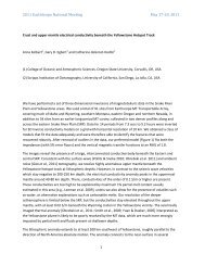
Section 4 – Using <strong>Surface</strong> <strong>Wave</strong>s <strong>to</strong> Build a Global Model<br />
We present an example from a current research project:<br />
“LITHO1.0 – <strong>An</strong> updated crust and lithospheric model<br />
of the Earth developed using multiple data constraints”<br />
<strong>Michael</strong> E. <strong>Pasyanos</strong> (LLNL)<br />
Guy Masters, Gabi Laske and Zhitu Ma (IGPP, UC San Diego)<br />
This section is a modified version of a talk that we gave at the Fall 2012<br />
AGU Meeting in San Francisco
<strong>Introduction</strong><br />
Crustal models like CRUST5.1 (Mooney et al., 1998) and successor models like CRUST2.0<br />
(Bassin et al., 2000) have been well-utilized in the seismological and geophysical communities<br />
(e.g. CRUST5.1 has 474 citations in Web of Science 11/2012)<br />
Useful <strong>to</strong> varied sections of the communities<br />
• global <strong>to</strong>mography in order <strong>to</strong> remove the crustal “noise” <strong>to</strong> see the mantle “signal”<br />
• smaller scale crustal studies as starting model or comparison model<br />
Downsides<br />
• Poor predic<strong>to</strong>r of travel times<br />
• Resolution poor for many applications<br />
• Model is of questionable quality in many poorly-covered regions<br />
We are creating a 1 degree model of the crust and upper mantle that is consistent with<br />
• Our extensive knowledge on sedimentary basins<br />
• Improved information on crustal thickness<br />
• Upper mantle velocities from regional travel times (e.g. Pn, Sn)<br />
• High-resolution surface wave models across a broad frequency band<br />
Our goal is <strong>to</strong> develop a higher-resolution model that extends deeper in<strong>to</strong> the<br />
mantle <strong>to</strong> include the lithospheric lid. This is the LITHO1.0 model
Method<br />
Our philosophy is <strong>to</strong> test a large series of models which are perturbations of a starting model<br />
which is consistent with other information about crust and upper mantle structure (e.g. tec<strong>to</strong>nic<br />
regions, crustal thickness from receiver functions and other information, upper mantle velocities<br />
from travel time models, thermo-tec<strong>to</strong>nic information, etc.)<br />
There is a balance between honoring prior information and allowing enough variation <strong>to</strong> fit the<br />
surface wave data<br />
Starting model<br />
- Honors prior information<br />
- Model may be poor<br />
- Doesn’t allow sufficient variations<br />
- Often doesn’t fit surface wave data<br />
<strong>Surface</strong> <strong>Wave</strong>s<br />
- Provides varied models<br />
- More sensitive <strong>to</strong> bulk properties, rather<br />
than discontinuities<br />
- Doesn’t honor prior information<br />
- Important for global <strong>to</strong>mography models
Parameterization<br />
Lateral Parameterization is achieved through tessellated nodes<br />
Depth parameterization through the thickness and associated parameters of layers<br />
Layer Layer Name Associated Parameters<br />
W Water/Ice thick, vp, vs, density, Qp, Qs<br />
S1 Sediment Layer 1 thick, vp, vs, density, Qp, Qs<br />
S2 Sediment Layer 2 thick, vp, vs, density, Qp, Qs<br />
S3 Sediment Layer 3 thick, vp, vs, density, Qp, Qs<br />
C1 Upper Crust thick, vp, vs, density, Qp, Qs<br />
C2 Middle Crust thick, vp, vs, density, Qp, Qs<br />
Level 1 = 12 nodes at ~60° resolution<br />
Level 2 = 42 nodes at ~30° resolution<br />
Level 3 = 162 nodes at ~15° resolution<br />
Level 4 = 642 nodes at ~8° resolution<br />
Level 5 = 2562 nodes at ~4° resolution<br />
Level 6 = 10,242 nodes at ~2° resolution<br />
Level 7 = 40,962 nodes at ~1° resolution<br />
C3 Lower Crust thick, vp, vs, density, Qp, Qs<br />
M1 Lithospheric Lid thick, vp, vs, density, Qp, Qs<br />
M2 Asthenosphere thick, vp, vs, density, Qp, Qs<br />
M3 Upper Mantle thick, vp, vs, density, Qp, Qs
Building the starting model<br />
CRUST1.0 pro<strong>to</strong>type<br />
- Modified CRUST2.0 crustal model at higher resolution<br />
- Full three-layer sediment model (Laske and Masters, 1997)<br />
- Updated crustal thickness map<br />
Upper mantle velocities from LLNL-G3Dv3 derived from<br />
regional and teleseismic travel times (Simmons et al., 2012)<br />
Lithospheric thickness from the regression of long period<br />
dispersion and lithospheric thickness estimates from heat flow<br />
(continents) and lithospheric cooling (oceans) (<strong>Pasyanos</strong>, 2005)<br />
Transitioned in<strong>to</strong> ak135 model (Kennett et al., 1995) at depth<br />
U80s (km/s)<br />
Lithospheric thickness (km)
Varying the starting model<br />
After creating an initial model, we perturb a number of model parameters (crustal<br />
velocities, mantle velocities, crustal thickness, lid thickness) <strong>to</strong> create a suite of<br />
about 10,000 models.<br />
Water/ice/sediment structure – fixed<br />
Crustal velocity stack – perturbed (±5%)<br />
Crustal thickness – varied (±1.5 σ)<br />
Upper mantle velocity – perturbed (±3%)<br />
Lithospheric thickness – varied (±1.5 σ)<br />
Transitioned in<strong>to</strong> ak135 model<br />
v p /v s fixed in seds/crust from CRUST1.0<br />
set for lid, astheno<br />
fixed from ak135 in mantle<br />
The dispersion values predicted by each model are then calculated using MINOS<br />
and compared <strong>to</strong> the observed dispersion from our high-resolution global surface<br />
wave model.<br />
We select the model that fits the observed dispersion the best
Example – node 14675<br />
The range of models covers the parameter<br />
space in both depth space and dispersion<br />
space<br />
For this node, we are able <strong>to</strong> fit the surface<br />
waves with a faster crust, a slightly faster<br />
mantle, a thicker crust, and a thinner<br />
lithospheric thickness
We assemble the results <strong>to</strong> construct the full model –<br />
Global, low-resolution, starting model<br />
Tessellation Level 5<br />
(~4°)
We assemble the results <strong>to</strong> construct the full model –<br />
Global, low-resolution, inverted model<br />
Tessellation Level 5<br />
(~4°)
High-resolution regional results for the Middle East<br />
Tessellation Level 7<br />
(~1°)
Depth slices through the model<br />
5 km<br />
10 km<br />
25 km
Depth slices through the model<br />
50 km<br />
75 km<br />
100 km
Close relationship between surface wave model and LITHO1.0<br />
100 s Rayleigh wave group vel<br />
75 km depth slice
High-resolution regional results for Siberia<br />
Tessellation Level 7<br />
(~1°)<br />
Constraints on lithospheric thickness can be used <strong>to</strong><br />
provide information on the Siberian Shield and study<br />
the nature of this diffuse plate boundary between<br />
the Eurasia and North American Plates and the<br />
interaction with the Amur and Okhotsk Plates
High-resolution regional results for North America<br />
PACIFIC<br />
OCEAN<br />
COAST<br />
RANGES<br />
GREAT<br />
BASIN<br />
COLORADO<br />
PLATEAU<br />
GREAT<br />
PLAINS<br />
This is a fully 3D model with<br />
parameters at all points in the<br />
model
The resulting model recovers the dispersion signal over a wide<br />
frequency range<br />
Starting model Inverted Model Data<br />
Rayleigh wave<br />
Phase Velocity<br />
20 mHz / 50 sec<br />
Starting model Inverted Model Data<br />
Rayleigh wave<br />
Group Velocity<br />
30 mHz / ~33 sec
LITHO1.0 - Summary and Future Work<br />
The LITHO1.0 model appears <strong>to</strong> both fit the surface wave data and be consistent<br />
with other geophysical information and tec<strong>to</strong>nic structure<br />
We would like <strong>to</strong> validate this more rigorously with travel time, waveform, and<br />
other data<br />
Finish the model<br />
§ We may still need <strong>to</strong> tweak the inversion <strong>to</strong> make crustal thickness changes<br />
smaller or convince ourselves that they are real<br />
§ We will incorporate anisotropy by allowing for a transversely isotropic mantle<br />
(in lid and asthenosphere)<br />
§ Make the runs at Tessellation Level 7 (~ 1°) globally<br />
Make the model and interfaces available<br />
§ Create model in other formats (e.g. regular lat/lon grid, spherical harmonics?)<br />
from native tessellation format <strong>to</strong> be usable <strong>to</strong> the widest array of users<br />
§ Supply interfaces <strong>to</strong> provide depth profiles at arbitrary lat/lon locations and<br />
parameters (e.g. V P , V S , etc.) at arbitrary lat/lon/depth points.