USP Analysis of Biological Assays - IPQ

1
2
3
4
5
6
7
8
9
10
11
12
13
14
15
16
17
18
19
20
21
22
23
24
25
26
27
28
29
30
31
32
33
34
35
36
37
38
39
40
41
42
43
44
45
46
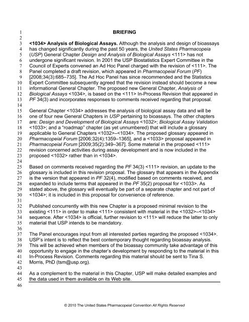
BRIEFING
Analysis of Biological Assays. Although the analysis and design of bioassays
has changed significantly during the past 50 years, the United States Pharmacopeia
(USP) General Chapter Design and Analysis of Biological Assays has not
undergone significant revision. In 2001 the USP Biostatistics Expert Committee in the
Council of Experts convened an Ad Hoc Panel charged with the revision of . The
Panel completed a draft revision, which appeared in Pharmacopeial Forum (PF)
[2008;34(3):685–735]. The Ad Hoc Panel has since recommended and the Statistics
Expert Committee subsequently agreed that the revision instead should become a new
informational General Chapter. The proposed new General Chapter, Analysis of
Biological Assays , is based on the In-Process Revision that appeared in
PF 34(3) and incorporates responses to comments received regarding that proposal.
General Chapter addresses the analysis of biological assay data and will be
one of four new General Chapters in USP pertaining to bioassays. The other chapters
are: Design and Development of Biological Assays ; Biological Assay Validation
; and a “roadmap” chapter (as yet unnumbered) that will include a glossary
applicable to General Chapters –. The proposed glossary appeared in
Pharmacopeial Forum [2006;32(4):1359–1365], and a proposal appeared in
Pharmacopeial Forum [2009;35(2):349–367]. Some material in the proposed
revision concerned activities during assay development and is now included in the
proposed rather than in .
Based on comments received regarding the PF 34(3) revision, an update to the
glossary is included in this revision proposal. The glossary that appears in the Appendix
is the version that appeared in PF 32(4), modified based on comments received, and
expanded to include terms that appeared in the PF 35(2) proposal for . As
stated above, the glossary will eventually be part of a separate chapter and not part of
; it is included in this proposal for convenience of reference.
Published concurrently with this new Chapter is a proposed minimal revision to the
existing in order to make consistent with material in the –
sequence. After is official, further revision to will reduce the latter to only
material that USP intends to be mandatory.
The Panel encourages input from all interested parties regarding the proposed .
USP’s intent is to reflect the best contemporary thought regarding bioassay analysis.
This will be achieved when members of the bioassay community take advantage of this
opportunity to engage in the chapter’s development by responding to the material in this
In-Process Revision. Comments regarding this material should be sent to Tina S.
Morris, PhD (tsm@usp.org).
As a complement to the material in this Chapter, USP will make detailed examples and
the data used in them available on its Web site.
© 2010 The United States Pharmacopeial Convention All Rights Reserved

47
48
49
50
51
52
53
54
55
56
57
58
59
60
61
62
63
64
65
66
67
68
69
70
71
72
73
74
75
76
77
78
79
80
81
82
83
84
85
86
87
88
89
90
91
92
ANALYSIS OF BIOLOGICAL ASSAYS
1. INTRODUCTION
Although advances in chemical characterization have reduced the reliance on
bioassays for many products, bioassays are still essential for the determination of
potency and the assurance of activity of many proteins, vaccines, cell therapy, gene
therapy, and complex mixtures, as well as for their role in monitoring the stability of
biological products. The intended scope of General Chapter Analysis of Biological
Assays includes guidance for the analysis of results both of bioassays
described in the United States Pharmacopeia (USP), and of non-USP bioassays that
seek to conform to the qualities of bioassay analysis recommended by USP. Note the
emphasis on analysis—design and validation are addressed in complementary chapters
( and , respectively).
Topics addressed in include statistical concepts and methods of analysis for the
calculation of potency and confidence intervals for a variety of relative potency
bioassays, including those referenced throughout USP. Chapter is intended for
use primarily by those who do not have extensive training or experience in statistics and
by statisticians who are not experienced in the analysis of bioassays. Sections that are
primarily conceptual require only minimal statistics background. Most of the Chapter
and all the methods sections require that the nonstatistician be comfortable with
statistics at least at the level of USP General Chapter Analytical Data—Interpretation
and Treatment and with linear regression. Most of Sections 3.4 and 3.6 require
more extensive statistics background and thus are intended primarily for statisticians. In
addition, introduces selected complex methods, the implementation of which
requires the guidance of an experienced statistician.
Approaches in are recommended, recognizing the possibility that alternative
procedures may be employed. Additionally, the information in is presented
assuming that computers and suitable software will be used for data analysis. This view
does not relieve the analyst of responsibility for the consequences of choices pertaining
to bioassay design and analysis.
2. OVERVIEW OF ANALYSIS OF BIOASSAY DATA
Following is a set of steps that will help guide the analysis of a bioassay. This Section
presumes that decisions were made following a similar set of steps during development,
checked during validation, and then not required routinely. Those steps and decisions
are covered in General Information Chapter Design and Development of Biological
Assays . Section 3 provides details for the various models considered.
(1) As a part of the chosen analysis, select the subset of data to be used in the
determination of the relative potency using the prespecified scheme. Exclude
only data known to result from technical problems such as contaminated wells,
non-monotonic concentration–response curves, etc.
© 2010 The United States Pharmacopeial Convention All Rights Reserved

93
94
95
96
97
98
99
100
101
102
103
104
105
106
107
108
109
110
111
112
113
114
115
116
117
118
119
120
121
122
123
124
125
126
127
128
129
130
131
132
133
134
135
136
137
(2) Fit the statistical model for detection of potential outliers, as chosen during
development, including any weighting and transformation. This is done first
without assuming similarity of the Test and Standard curves but should include
important elements of the design structure, ideally using a model that makes
fewer assumptions about the functional form of the response than the model
used to assess similarity.
(3) Determine which potential outliers are to be removed and fit the model to be
used for suitability assessment. Usually, an investigation of outlier cause takes
place before outlier removal. Some assay systems can make use of a statistical
(noninvestigative) outlier removal rule, but removal on this basis should be rare.
(4) Assess system suitability. System suitability assesses whether the assay
Standard preparation and any controls behaved in a manner consistent with past
performance of the assay. If an assay (or a run) fails system suitability, the entire
assay (or run) is discarded and no results are reported other than that the assay
(or run) failed. Assessment of system suitability usually includes adequacy of the
fit of the model used to assess similarity. For linear models, adequacy of the
model may include assessment of the linearity of the Standard curve. If the
suitability criterion for linearity of the Standard is not met, the exclusion of one or
more extreme concentrations may result in the criterion’s being met. Examples of
other possible system suitability criteria include background, positive controls,
max/min, max/background, slope, EC 50 (or ED 50 ), and variation around the fitted
model.
(5) Assess sample suitability for each Test sample. This is done to confirm that the
data for each Test sample satisfy necessary assumptions. If a Test sample fails
sample suitability, results for that sample are reported as “Fails.” Relative
potencies for other Test samples in the assay may still be reported. Most
prominent of sample suitability criteria is similarity, whether parallelism for
parallel models or equivalence of intercepts for slope-ratio models. For nonlinear
models, similarity assessment involves all curve parameters other than ED 50 (or
IC 50 ).
(6) For those Test samples in the assay that meet the criterion for similarity to the
Standard (i.e., sufficiently similar concentration–response curves or similar
straight-line subsets of concentrations), calculate relative potency estimates
assuming similarity between Test and Standard, i.e., assuming exactly parallel
lines or curves or equal intercepts.
(7) A single assay is often not sufficient to achieve a reportable value, and potency
results from multiple assays can be combined into a single potency estimate.
Repeat steps 1–6 multiple times, as specified in the assay protocol or
monograph, before determining a final estimate of potency and a confidence
interval.
(8) Construct a variance estimate and confidence interval for the estimated potency
of the analyte. See Section 4.
A step that is not shown concerns replacement of missing data. Most modern statistical
methodology (and software) does not require equal numbers at each combination of
© 2010 The United States Pharmacopeial Convention All Rights Reserved

138
139
140
141
142
143
144
145
146
147
148
149
150
151
152
153
154
155
156
157
158
159
160
161
162
163
164
165
166
167
168
169
170
171
172
173
174
175
176
177
178
179
180
181
182
183
concentration and sample. Thus, unless otherwise directed by a specific monograph,
analysts generally do not need to replace missing values.
3. ANALYSIS MODELS
A number of mathematical functions can be successfully used to describe a
concentration–response relationship. The first consideration in choosing a model is the
form of the assay response. Is it a number, a count, or a category such as dead/alive?
The form will identify the possible models that can be considered.
Other considerations in choosing a model include the need to incorporate design
elements in the model and the possible benefits of means models compared to
regression models. For purposes of presenting the essentials of the model choices,
Section 3 assumes a completely randomized design so that there are no design
elements to consider and presents the models in their regression form. See examples
on the USP Web site that incorporate design elements and contrast means models to
regression models.
3.1 Quantitative and Qualitative Assay Responses
The terms quantitative and qualitative refer to the nature of the response of the assay
used in constructing the concentration–response model. Assays with either quantitative
or qualitative responses can be used to quantify product potency. Note that the
responses of the assay at the concentrations measured are not the relative potency of
the bioassay. Analysts should understand the differences among responses,
concentration–response functions, and relative potency.
A quantitative response results in a number on a continuous scale. Common examples
include spectrophotometric and luminescence responses, body weights and
measurements, and data calculated relative to a standard curve (e.g., cytokine
concentration). Models for quantitative responses can be linear or nonlinear (see
Sections 3.2–3.5).
A qualitative measurement results in a categorical response. For bioassay, qualitative
responses are most often quantal, meaning they entail two possible categories such as
Positive/Negative, 0/1, or Dead/Alive. Quantal responses may be reported as
proportions (e.g., the proportion of animals in a group displaying a property). Quantal
models are presented in Section 3.6. Qualitative responses can have more than two
possible categories, such as end-point titer assays. Models for more than two
categories are not considered in this General Chapter.
Assay responses can also be counts, such as number of plaques or colonies. Integer
responses are sometimes treated as quantitative, sometimes as qualitative, and
sometimes models specific to integers are used. The choice is often based on the range
of counts. If the count is mostly 0 and rarely greater than 1, the assay may be analyzed
as quantal and the response is Any/None. If the counts are large and cover a wide
© 2010 The United States Pharmacopeial Convention All Rights Reserved

184
185
186
187
188
189
190
191
192
193
194
195
196
197
198
199
200
201
202
203
204
205
206
207
208
209
210
211
212
213
214
215
216
217
218
219
220
221
222
223
224
225
226
227
228
range, such as 500 to 2500, then the assay may be analyzed as quantitative, possibly
after transformation of the counts. A square root transformation of the count is often
helpful in such analyses to better satisfy homogeneity of variances. If the range of
counts includes or is near 0 but 0 is not the preponderant value, it may be preferable to
use a model specific for integer responses. Poisson regression and negative binomial
regression models are often good options. Models specific to integers will not be
discussed further in this General Chapter.
Assays with quantitative responses may be converted to quantal responses. For
example, what may matter is whether some defined threshold is exceeded. The model
could then be quantal—threshold exceeded or not. In general, assay systems have
more precise estimates of potency if the model uses all the information in the response.
Using above or below a threshold, rather than the measured quantitative responses, is
likely to degrade the performance of an assay.
3.2 Overview of Models for Quantitative Responses
In quantitative assays, the measurement is a number on a continuous scale. Optical
density values from plate-based assays are such measurements. Models for
quantitative assays can be linear or nonlinear. Although the two display an apparent
difference in levels of complexity, parallel-line (linear) and parallel-curve (nonlinear)
models share many commonalities. Because of the different form of the equations,
slope-ratio assays are considered separately (Section 3.5).
Assumptions. The basic parallel-line, parallel-curve, and slope-ratio models share
some assumptions. All include a residual term, e, which is assumed to be independent
from measurement to measurement and to have constant variance from concentration
to concentration. Often the residual term is assumed to have a normal distribution as
well. The assumptions of independence and equal variances are commonly violated, so
the goal in analysis is to incorporate the lack of independence and the unequal
variances into the statistical model or the method of estimation.
Lack of independence often arises because of the design or conduct of the assay. For
example, if the assay consists of responses from multiple plates, observations from the
same plate are likely to share some common influence that is not shared with
observations from other plates. This is an example of intraplate correlation. A simple
approach for dealing with this lack of independence is to include a block term in the
statistical model for plate. With three or more plates this should be a random effects
term so that we obtain an estimate of plate-to-plate variability.
In general, the model needs to closely reflect the design. The basic model equations
given in Sections 3.3–3.5 apply only to completely randomized designs. Any other
design will mean additional terms in the statistical model. For example, if plates or
portions of plates are used as blocks, one will need terms for blocks.
© 2010 The United States Pharmacopeial Convention All Rights Reserved

229
230
231
232
233
234
235
236
237
238
239
240
241
242
243
244
245
246
247
248
249
250
251
252
253
254
255
256
257
258
259
260
261
262
263
264
265
266
267
268
269
270
271
272
273
274
Calculation of potency. A primary assumption underlying methods used for the
calculation of relative potency is that of similarity. Two preparations are similar if they
contain the same effective constituent or same effective constituents in the same
proportions. If this condition holds, the Test preparation behaves as a dilution (or
concentration) of the Standard preparation. Similarity can be represented
mathematically as follows. Let F T be the concentration–response function for the Test,
and let F S be the concentration–response function for the Standard. The underlying
mathematical model for similarity is:
F T (z) = F S (ρ z), [3.1]
where z represents the concentration and ρ represents the relative potency of the Test
sample relative to the Standard sample.
Methods for estimating ρ in some common concentration–response models are
discussed below. For linear models, the distinction between parallel-line models
(Section 3.3) and slope-ratio models (Section 3.5) is based on whether a straight-line fit
to log concentration or concentration yields better agreement between the model and
the data over the range of concentrations of interest.
3.3 Parallel-line Models for Quantitative Responses
In this section, a linear model refers to a concentration–response relationship, which is
a straight-line (linear) function between the logarithm of concentration, X, and the
response, Y. Y may be the response in the scale as measured or a transformation of
the response. The functional form of this relationship is Y = a + bX. Straight-line fits may
be used for portions of nonlinear concentration–response curves, although doing so
requires a method for selecting the concentrations to use for each of Standard and Test
samples (see ).
Means models vs regression. A linear concentration–response model is (outside
bioassay) most often analyzed with ordinary least squares regression. Such an analysis
results in estimates of the unknown coefficients (intercepts and slope) and their
standard errors, as well as measures of the goodness of fit [e.g., R 2 or root-meansquare
error (RMSE)].
Linear regression works best where all concentrations can be used and there is
negligible curvature in the concentration–response data. Another statistical method for
analyzing linear concentration–response curves is the means model. This is an analysis
of variance (ANOVA) method that offers some advantages, particularly when one or
more concentrations from one or more samples are not used to estimate potency.
Because a means model uses all observations to measure variation, it will capture the
variance in the bioassay system better than a regression model does. A means model
contains a saturated model for samples crossed with concentrations, where
concentrations are treated as a categorical variable (class or factor) rather than as a
regression predictor. That is, the model includes a term for each combination of
concentration and sample. With a means model, straight lines are fit to test and
reference using linear combinations of the fitted means.
© 2010 The United States Pharmacopeial Convention All Rights Reserved

275
276
277
278
279
280
281
282
283
284
285
Parallel-line concentration–response models. If the general concentration–response
model (3.1) can be made linear in x = log(z), the resulting equation is then:
y = α + β log(z) + e = α + βx + e,
where the intercept, α, and slope, β, will differ between Test and Standard. With the
parallelism (equal slopes) assumption, the model becomes
yS
=α+β log(z) + e =α
S
+β x + e
[3.2]
y =α+βlog( ρ z) + e = [ α+βlog( ρ )] +β x + e =α +β x + e
T
where S denotes Standard, T denotes Test, α S = α is the y-intercept for the Standard,
and α T = α + βlog(ρ) is the y-intercept for the Test (see Figure 3.1).
Figure 3.1. Example of parallel-line model
T
Assay Response
Standard
286
287
288
289
290
291
292
293
294
295
296
297
298
299
300
301
302
303
304
305
log 10 Concentration
Where concentration–response lines are parallel, as shown in Figure 3.1, a separation
or horizontal shift in one line indicates a difference in the level of biological activity being
assayed. This horizontal difference is numerically log(ρ), the logarithm of the relative
potency, and is found as the vertical distance between the lines α T and α S divided by
the slope, β. The relative potency is then
⎛ αT
−αS
⎞
ρ= antilog ⎜ ⎟
⎝ β ⎠
Estimation of parallel-line models. Parallel-line models are fit by the method of least
squares. If the equal variance assumption holds, the parameters of [3.2] are chosen to
minimize
2
y − αˆ −δˆT −βˆx [3.3]
∑
( S )
where the carets denote estimates. This is a linear regression with two independent
variables, T and x, where T is a variable that equals 1 for observations from the Test
and 0 for observations from the Standard. The summation in [3.3] is over all
observations of the Test and Standard. If the equal variance assumption does not hold
but the variance is known to be inversely proportional to a value, w, that does not
depend on the current responses, the y’s, and can be determined for each observation,
then the method is weighted least squares
2
w y − αˆ −δˆT −βˆx [3.4]
∑
( S )
© 2010 The United States Pharmacopeial Convention All Rights Reserved

306
307
308
309
310
311
312
313
314
315
316
317
318
319
320
321
322
323
324
325
326
327
328
329
330
331
332
333
334
335
336
337
338
339
340
341
342
343
344
345
Equation 3.4 is appropriate only if the weights are determined without using the
response, the y’s, from the current data (see for guidance in determining
weights). In [3.3] and [3.4] β is the same as the β in [3.2] and δ = α T – α S = β log ρ. So,
the estimate of the relative potency, ρ, is
⎛ δ ⎞
ρ= ˆ antilog
ˆ
⎜
β
⎟
⎝
ˆ
⎠
Commonly available statistical software and spreadsheets provide routines for least
squares. Not all software can provide weighted analyses.
Measurement of nonparallelism. Parallelism for linear models is assessed by
considering the difference or ratio of the two slopes. For the difference, this is can be
done by fitting the regression model,
y = α S + δT + β S x + γxT + e
where δ = α T − α S , γ = β T − β S , and T = 1 for Test data and T = 0 for Standard data. Then
use the standard t-distribution confidence interval for γ. For the ratio of slopes, fit
y = α S + δT + β S x + β T x + e
and use Fieller’s Theorem [4.3] to obtain a confidence interval for β T /β S .
3.4 Nonlinear Models for Quantitative Responses
Nonlinear concentration–response models are typically S-shaped functions. They occur
when the range of concentrations is wide enough so that responses are constrained by
upper and lower asymptotes. The most common of these models is the four-parameter
logistic function as given below.
Let y denote the observed response and z the concentration. One form of the fourparameter
logistic model is
A−
D
y = D+ + e
B
z
1+
One alternative, but equivalent, form is
d
y = a0
+ + e
1+ antilog⎡⎣M ( logz −b)
⎤⎦
The two forms correspond as follows:
Lower asymptote: D = a 0
Upper asymptote: A = a 0 + d
Steepness: B = M (related to the slope of the curve at the EC 50 )
Effective concentration 50% (EC 50 ): C = antilog(b) (may also be termed ED 50 ).
Any convenient base for logarithms is suitable; it is often convenient to work in log base
2, particularly when concentrations are twofold apart.
The four-parameter logistic curve is symmetric around the EC 50 when plotted against
log concentration because the rates of approach to the upper and lower asymptotes are
the same (see Figure 3.2). For assays where this symmetry does not hold, a number of
( )
C
[3.5]
© 2010 The United States Pharmacopeial Convention All Rights Reserved

346
347
348
349
models for sigmoid curves are asymmetric, and these models are not considered further
in this General Chapter.
Figure 3.2. Examples of symmetric (four-parameter logistic) and asymmetric sigmoids
Symmetric
Asymmetric
350
351
352
353
354
355
356
357
358
359
360
361
362
363
364
365
366
367
368
369
370
371
372
373
In many assays the analyst has a number of strategic choices. For example, the
responses could be modeled using a transformed response fit to a four-parameter
logistic curve, or the responses could be weighted and fit to an asymmetric sigmoid
curve. Also, it is often important to include terms in the model (often random effects) to
address variation in the responses (or parameters of the response) associated with
blocks or experimental units in the design of the assay. For simple assays where
observations are independent, these strategic choices are fairly straightforward. For
assays performed with grouped dilutions (as with multichannel pipettes), assays with
serial dilutions, or assay designs that include blocks (as with multiple plates/assay), it is
usually a more serious violation of the statistical assumptions to ignore the design
structure than to use a transformation that approximates a solution to nonconstant
variance and asymmetry. Additionally, for these more complex assays, such
transformation is superior to imposing a weighted fit to an asymmetric model.
Parallel-curve Concentration–Response Models. The concept of parallelism is not
restricted to linear models. For nonlinear curves, parallel or similar means the
concentration–response curves can be superimposed following a horizontal
displacement of one of the curves, as shown in Figure 3.3 for four-parameter logistic
curves. In terms of the parameters of [3.5], this means the values of A, D, and B for the
Test are the same as for the Standard.
© 2010 The United States Pharmacopeial Convention All Rights Reserved

374
Figure 3.3. Example of parallel curves from a nonlinear model
Assay Response
375
376
377
378
379
380
381
382
383
384
385
386
387
388
389
390
391
392
393
394
log 10 Concentration
The equations corresponding to the figure (with error term, e, added) are
A−
D
yS
= D+ + e
B
z
1+
( )
A−
D
yT
= D+ + e
B
1+
or
A−
D
yS
= D+ + e
1+ antilog⎡⎣M ( logz −b)
⎤⎦
A−
D
yT
= D+ + e
1+ antilog⎡⎣M ( logz − b + logρ)
⎤⎦
Log ρ is the log of the relative potency and the horizontal distance between the two
curves, just as for the parallel-line model. Because the EC50 of the standard is
antilog(b) and that of the Test is antilog(b – log ρ) = antilog(b)/ρ, the relative potency is
the ratio of EC50’s (standard over Test) when the parallel-curve model holds.
Estimation of parallel-curve models. Estimation of nonlinear, parallel-curve models is
similar to that for parallel-line models, possibly after transformation of the response and
possibly with weighting. For the four-parameter logistic model, the parameter estimates
are found by minimizing:
without weighting, or
∑
C
ρz
( C )
⎛
⎞
⎜ Aˆ
− Dˆ
y−Dˆ
−
⎟
⎜
1+ antilog⎡Mˆ ( logz − bˆ + rT ˆ ) ⎤ ⎟
⎝
⎣
⎦ ⎠
⎛
⎞
⎜ Aˆ
− Dˆ
− −
⎟
∑ w y Dˆ
[3.6]
⎜
1+ antilog⎡Mˆ ( logz − bˆ + rT ˆ ) ⎤ ⎟
⎝
⎣
⎦ ⎠
with weighting. (As for Equation 3.4, [3.6] is appropriate only if the weights are
determined without using the responses, y’s, from the current data.) In either case, the
2
2
© 2010 The United States Pharmacopeial Convention All Rights Reserved

395
396
397
398
399
400
401
402
403
404
405
406
407
408
409
410
411
412
413
414
415
416
417
418
419
420
421
422
423
424
425
426
427
428
429
430
431
432
estimate of r is the estimate of the log of the relative potency. For some software, it may
be easier to work with a 0 = A – D.
The parameters of the four-parameter logistic function and those of the asymmetric
sigmoid models cannot be found with ordinary (linear) least squares regression
routines. Computer programs with nonlinear estimation techniques must be used.
Analysts should not use the nonlinear regression fit to assess parallelism or estimate
potency if any of the following are present: a) inadequate asymptote information is
available; or b) a comparison of pooled error(s) from nonlinear regression to pooled
error(s) from a means model shows that the nonlinear model does not fit well; or c)
other appropriate measures of goodness of fit show that the nonlinear model is not
appropriate (e.g., residual plots show evidence of a “hook”).
Measurement of nonparallelism. Assessment of parallelism for a four-parameter
logistic model means assessing the slope parameter and the two asymptotes. During
development (see ), a decision should be made regarding which parameters are
important and how to measure nonparallelism. As discussed in , the measure of
nonsimilarity may be a composite measure that considers all parameters together in a
single measure or may consider each parameter separately. In the latter case, the
measure may be functions of the parameters, such as an asymptote divided by the
difference of asymptotes. For each parameter (or function of parameters), confidence
intervals can be computed by bootstrap or likelihood profile methods. These methods
are not presented in this General Chapter.
3.5 Slope-ratio Concentration–Response Models
If a straight-line regression fits the nontransformed concentration–response data well, a
slope-ratio model may be used. The equations for the slope-ratio model assuming
similarity are then:
yS
=α+β x+ e=α+β Sx+
e
[3.7]
y
T
=α+βρ ( x) + e = α+βSρ x+ e=α+β Tx+
e
An identifying characteristic of a slope-ratio concentration–response model that can be
seen in the results of a ranging study is that the lines for different potencies from a
ranging study have the same intercept and different slopes. Thus, a graph of the
ranging study resembles a fan. Figure 3.4 shows an example of a slope-ratio
concentration–response model. Note that the common intercept need not be the origin.
© 2010 The United States Pharmacopeial Convention All Rights Reserved

433
Figure 3.4. Example of slope ratio model
Assay Response
Standard
Test
434
435
436
437
438
439
440
441
442
443
444
445
446
447
448
449
450
451
452
453
454
455
456
457
458
459
460
461
462
463
Concentration
An assay with a slope-ratio concentration–response model for measuring relative
potency consists, at a minimum, of one Standard sample and one Test sample, each
measured at one or more concentrations and, usually, a measured response with no
sample (zero concentration). Because the concentrations are not log transformed, they
are typically equally spaced on the original, rather than log, scale. The model consists of
one common intercept, a slope for the Test sample results, and a slope for the Standard
sample results as in [3.7]. The relative potency is then found from the ratio of the
slopes:
Test sample slope βρ
Relative Potency = = =ρ
Standard sample slope β
Assumptions for and estimation of slope-ratio models. The assumptions for the
slope-ratio model are the same as for parallel-line models: The residual terms are
independent, have constant variance, and may need to have a normal distribution. The
method of estimation is also least squares. This may be implemented either with or
without weighting, as demonstrated in equations [3.8] and [3.9], respectively.
2
y −α−β ˆ ˆ x(1−T) −βˆ
xT [3.8]
∑
∑
( S
T )
( −α−βˆ
S
− −βˆ
T )
2
w y ˆ x(1 T) xT [3.9]
Equation 3.9 is appropriate only if the weights are determined without using the
response, the y’s, from the current data. This is a linear regression with two
independent variables, x(1 – T) and xT, where T = 1 for Test data and T = 0 for
Standard data. βT
ˆ is the estimated slope for the Test, βS
ˆ the estimated slope for the
βˆ
Standard, and then the estimate of relative potency is R =
T
βˆ
.
Because the slope-ratio model is a linear regression model, most statistical packages
and spreadsheets can be used to obtain the relative potency estimate. In some assay
systems, it is sometimes appropriate to omit the zero concentration and at times one or
more of the high concentrations. The discussion about using a means model and
S
© 2010 The United States Pharmacopeial Convention All Rights Reserved

464
465
466
467
468
469
470
471
472
473
474
475
476
477
478
479
480
481
482
483
484
485
486
487
488
489
490
491
492
493
494
495
496
497
498
499
selecting subsets of concentrations for straight parallel-line bioassays applies to sloperatio
assays as well.
Measurement of nonsimilarity. For slope-ratio models, statistical similarity
corresponds to equal intercepts for the Standard and Test. To assess the similarity
assumption it is necessary to have at least two nonzero concentrations for each sample.
If the intercepts are not equal, [3.7] becomes
y S = α S + β S x + e
y T = α T + β T x + e
Departure from similarity is typically measured by the difference of intercepts, α T − α S .
An easy way to obtain a confidence interval is to fit the model,
y = α S + δT + β S x(1 – T) + β T xT + e,
where δ = α T − α S and use the standard t-distribution–based confidence interval for δ.
3.6 Dichotomous (Quantal) Assays
For quantal assays the assay measurement has a dichotomous or binary outcome, e.g.,
in animal assays the animal is dead or alive or a certain physiologic response is or is
not observed. For cellular assays, the quantal response may be whether there is or is
not a response beyond some threshold in the cell. In cell-based viral titer or colonyforming
assays, the quantal response may be a limit of integer response such as an
integer number of particles or colonies. When one can readily determine if any particles
are present—but not their actual number—then the assay can be analyzed as quantal.
Note that if the reaction can be quantitated on a continuous scale, as with an optical
density, then the assay is not quantal.
Models for quantal analyses. The key to models for quantal responses is to work with
the probability of a response (e.g., probability of death), in contrast to quantitative
responses for which the model is the response itself. For each concentration, d, a
treated animal, as an example, has a probability of responding to that concentration,
P(d). Often the curve P(d) can be approximated by a sigmoid when plotted against the
logarithm of concentration, as shown in Figure 3.5. This curve shows that the probability
of responding increases with concentration. The concentration that corresponds to a
probability of 0.5 is the ED 50 .
Figure 3.5. Example of sigmoid for P(d)
500
© 2010 The United States Pharmacopeial Convention All Rights Reserved

501
502
503
504
505
506
507
508
509
510
511
512
513
514
515
516
517
518
519
520
521
522
523
524
525
526
527
528
529
530
531
532
533
534
The sigmoid curve is usually modeled based on the normal or logistic distribution. If the
normal distribution is used, the resulting analysis is termed probit analysis, and if the
logistic is used the analysis is termed logit or logistic analysis. The probit and logit
models are practically indistinguishable, and either is an acceptable choice. The choice
may be based on the availability of software that meets the laboratory’s analysis and
reporting needs. Because software is more commonly available for logistic models
(often under the term logistic regression) this discussion will focus on the use and
interpretation of logit analysis. The considerations discussed in this section for logit
analysis (using a logit transformation) apply as well to probit analysis (using a probit
transformation).
Logit model. The logit model for the probability of response, P(d), can be expressed in
two equivalent forms. For the sigmoid,
1
P(d) =
1 + antilog[ −β −β log(d)]
1
=
+
1
1 d ED50
( ) −β
0 1
where log(ED50) = −β 0 /β 1 . An alternative form shows the relationship to linear models:
⎛ P ⎞
logit transform of P = log⎜
⎟=β 0
+β1log(d)
[3.10]
⎝1−
P⎠
The linear form is usually shown using natural logs and is a useful reminder that many
of the considerations, in particular linearity and parallelism, discussed for parallel-line
models in Section 3.3 apply to quantal models as well.
For a logit analysis with Standard and Test preparations, let T be a variable that takes
the value 1 for animals receiving the Test preparation and 0 for animals receiving the
Standard. Assuming parallelism of the Test and Standard curves, the logit model for
estimating relative potency is then:
⎛ P ⎞
log⎜
⎟= β
0
+β
1log(d) +β2T
⎝1−
P⎠
The log of the relative potency of the Test compared to the Standard preparation is then
β 2 /β 1 . The two curves in Figure 3.6 show parallel Standard and Test sigmoids. (If the
corresponding linear forms [3.10] were shown, they would be two parallel straight lines.)
The log of the relative potency is the horizontal distance between the two curves, in the
same way as for the linear and four-parameter logistic models given for quantitative
responses (Sections 3.4 and 3.5).
© 2010 The United States Pharmacopeial Convention All Rights Reserved

535
Figure 3.6. Example of Parallel Sigmoid Curves
Test
Standard
536
537
538
539
540
541
542
543
544
545
546
547
548
549
550
551
552
553
554
555
556
557
558
559
560
561
562
563
564
565
566
567
568
569
Estimating the model parameters and relative potency. Two methods are available
for estimating the parameters of logit and probit models: maximum likelihood and
weighted least squares. The difference is not practically important, and the laboratory
can accept the choice made by its software. The following assumes a general logistic
regression software program. Specialized software should be similar.
Considering the form of 3.10, one observes a resemblance to linear regression. There
are two independent variables, log(d) and T. For each animal, there is a yes/no
dependent variable, often coded as 1 for yes or response and 0 for no or no response.
Although bioassays are often designed with equal numbers of animals per
concentration, that is not a requirement of analysis. Utilizing the parameters estimated
by software, which include β 0 , β 1 , and β 2 and their standard errors, one obtains the
estimate of the natural log of the relative potency:
)
β
Estimate of log of relative potency = ) 2
β
1
Substituting the parameter estimates and their standard errors into Fieller’s Theorem
(see Section 4.3), one can calculate the model-based confidence interval for the log of
relative potency. The confidence interval for the relative potency is then
[antilog(L), antilog(U)], where [L, U] is the confidence interval for the log relative
potency.
Assumptions. In most cases, quantal analyses assume a standard binomial model with
independence of results from animal to animal. The binomial is a common choice of
distribution for dichotomous data. The key assumptions of the binomial are that at a
given concentration each animal treated at that concentration has the same probability
of responding and the results for any animal are independent from those of all other
animals. This basic set of assumptions can be violated in many ways. Foremost among
them is the presence of litter effects, where animals from the same litter tend to respond
more alike than do animals from different litters. Cage effects, in which the
environmental conditions or care rendered to any specific cage makes the animals from
that cage more or less likely to respond to experimental treatment, violates the same
equal-probability assumption. These assumption violations and others like them (that
could be a deliberate design choice) do not preclude the use of logit or probit models.
© 2010 The United States Pharmacopeial Convention All Rights Reserved

570
571
572
573
574
575
576
577
578
579
580
581
582
583
584
585
586
587
588
589
590
591
592
593
594
595
596
597
598
599
600
601
602
603
604
605
606
607
608
609
610
611
612
613
614
Still, they are indications that a more complex approach to analysis than that presented
here may be required (see ).
Checking assumptions. To assess parallelism, equation [3.10] may be modified as
follows:
⎛ P ⎞
log⎜
⎟=β 0
+β
1log(d) +β
2T +β3T * log(d)
⎝1−
P⎠
Here, β 3 is the difference of slopes between Test and Standard and should be
sufficiently small. [The T*log(d) term is known as an interaction term in statistical
terminology.] The measure of nonparallelism may also be expressed in terms of the
ratio of slopes, (β 1 +β 3 )/β 1 . For model-based confidence intervals for these measures of
nonparallelism, bootstrap or profile likelihood methods are recommended. These
methods are not covered in this General Chapter.
To assess linearity, it is good practice to start with a graphical examination. In
accordance with [3.10], this would be a plot of log[(y + 0.5)/(n − y + 0 .5)] against
log(concentration), where y is the total number of responses at the concentration and n
is the number of animals at that concentration. (The 0.5 corrections improve the
properties of this calculation as an estimate of log(P/(1 – P)).)The lines for Test and
Standard should be parallel straight lines as for the linear model in quantitative assays.
If the relationship is monotonic but does not appear to be linear, then the model in [3.10]
can be extended with other terms. For example, a quadratic term in log(concentration)
could be added: [log(concentration)] 2 . If concentration needs to be transformed to
something other than log concentration, then the quantal model analogue of slope-ratio
assays is an option. The latter is possible but sufficiently unusual that it will not be
discussed further in this General Chapter.
Outliers. Assessment of outliers is more difficult for quantal assays than for quantitative
assays. Because the assay response can be only yes or no, no individual response can
be unusual. What may appear to fall into the outlier category is a single response at a
low concentration or a single no-response at a high concentration. Assuming that there
has been no cause found (e.g., failure to properly administer the drug to the animal),
there is no statistical basis for distinguishing an outlier from a rare event.
Alternative methods. Alternatives to the simple quantal analyses outlined here may be
acceptable, depending on the nature of the analytical challenge. One such challenge is
a lack of independence among experimental units, as may be seen in litter effects in
animal assays. Some of the possible approaches that may be employed are
Generalized Estimating Equations (GEE), generalized linear models, and generalized
linear mixed-effects models. A GEE analysis will yield standard errors and confidence
intervals whose validity does not depend on the satisfaction of the independence
assumption.
There are also methods that make no particular choice of the model equation for the
sigmoid. A commonly seen example is the Spearman–Kärber method.
© 2010 The United States Pharmacopeial Convention All Rights Reserved

615
616
617
618
619
620
621
622
623
624
625
626
627
628
629
630
631
632
633
634
635
636
637
638
639
640
641
642
643
644
645
646
647
648
649
650
651
652
653
654
655
656
657
658
659
4. CONFIDENCE INTERVALS
A report of an assay result should include a measure of the uncertainty of that result.
This can be a standard error or a confidence interval. An interval (c, d) is a 95%
confidence interval for a parameter (e.g., relative potency) if 95% of such intervals upon
repetition of the experiment would include the actual value of the parameter. A
confidence interval may be interpreted as indicating values of the parameter that are
consistent with the data. This interpretation of a confidence interval requires that
various assumptions be satisfied. The interval width is sometimes used as a suitability
criterion without the confidence interpretation. In such cases the assumptions need not
be satisfied.
Confidence intervals can either be model-based or sample-based. A model-based
interval is based on the standard errors for each of the one or more estimates of log
relative potency that come from the analysis of a particular statistical model. Modelbased
intervals should be avoided if sample-based intervals are possible. Model-based
intervals require that the statistical model correctly incorporate all the effects and
correlations that influence the model’s estimate of precision. These include but are not
be limited to serial dilution and plate effects. Section 4.3 describes Fieller’s Theorem, a
commonly used model-based interval.
Sample-based methods combine independent estimates of log relative potency. Multiple
assays may arise because this was determined to be required during development and
validation or because the assay procedure fixes a maximum acceptable width of the
confidence interval and two or more independent assays may be needed to meet the
specified width requirement. Some sample-based methods do not require that the
statistical model correctly incorporate all effects and correlations. However, this should
not be interpreted as dismissing the value of addressing correlations and other factors
that influence within-assay precision. The within-assay precision is used in similarity
assessment and is a portion of the variability that is the basis for the sample-based
intervals. Thus minimizing within-assay variability to the extent practical is important.
Sample-based intervals are covered in Section 4.2.
4.1 Combining Results from Multiple Assays
In order to mitigate the effects of variability, analysts often find it necessary to replicate
independent bioassays and to combine their results to obtain a single reportable value.
During assay development and validation, analysts should evaluate whether it is useful
to combine the results of such assays and, if so, in what way to proceed.
There are two primary questions to address when considering how to combine results
from multiple assays:
Are the assays mutually independent?
© 2010 The United States Pharmacopeial Convention All Rights Reserved

660
661
662
663
664
665
666
667
668
669
670
671
672
673
674
675
676
677
678
679
680
681
682
683
684
685
686
687
688
689
690
691
692
693
694
695
696
697
698
699
700
701
702
703
704
705
A set of assays may be regarded as mutually independent when the responses
of one do not in any way depend on the distribution of responses of any of the
others. This implies that the random errors in all essential factors influencing the
result (for example, dilutions of the standard and of the preparation to be
examined or the sensitivity of the biological indicator) in one assay must be
independent of the corresponding random errors in the other assays. Assays on
successive days using the original and retained dilutions of the Standard,
therefore, are not independent assays. Similarly, if the responses, particularly the
potency, depend on other reagents that are shared by assays (e.g., cell
preparations), the assays may not be independent.
Assays need not be independent in order for analysts to combine results.
However, methods for independent assays are much simpler. Also, combining
dependent assay results may require assumptions about the form of the
correlation between assay results that may be, at best, challenging to verify.
Statistical methods are available for dependent assays, but they are not
presented in this General Chapter.
Are the results of the assays homogeneous?
Homogeneous results differ only because of random within-assay errors. Any
contribution from factors associated with intermediate precision precludes
homogeneity of results. Intermediate precision factors are those that vary
between assays within a laboratory and can include analyst, equipment, and
environmental conditions. There are statistical tests for heterogeneity, but lack of
statistically significant heterogeneity is not properly taken as assurance of
homogeneity and so no test is recommended. If analysts use a method that
assumes homogeneity, homogeneity should be assessed during development,
documented during validation, and monitored during ongoing use of the assay.
Additionally, before results from assays can be combined, analysts should consider the
scale on which that combination is to be made. In general, the combination should be
done on the scale for which the parameter estimates are approximately normally
distributed. Thus, for relative potencies based on a parallel-line or parallel-curve
method, the relative potencies are combined in the logarithm scale.
4.2 Combining Independent Assays (Sample-based Confidence Interval Methods)
Analysts can use several methods for combining the results of independent assays. A
simple method described below (Method 1) assumes a common distribution of relative
potencies across the assays and is recommended. A second procedure is provided and
may be useful if homogeneity of relative potency across assays can be documented. A
third alternative is useful if the assumptions for Methods 1 and 2 are not satisfied.
Another alternative, analyzing all assays together using a linear or nonlinear mixedeffects
model, is not discussed in this General Chapter.
© 2010 The United States Pharmacopeial Convention All Rights Reserved

706
707
708
709
710
711
712
713
714
715
716
717
718
719
720
721
722
723
724
725
726
727
728
729
730
731
732
733
734
735
736
737
738
739
740
741
742
743
744
Method 1—independent assay results from a common assay distribution. The
following is a simple method that assumes independence of assays. It is assumed that
the individual assay results (logarithms of relative potencies) are from a common normal
distribution with some nonzero variance. This common distribution assumption requires
that all assays to be combined used the same design and laboratory procedures.
Implicit is that the relative potencies may differ between the assays. This method thus
captures interassay variability in relative potency. Note that the individual relative
potencies should not be rounded before combining results.
Let R i denote the logarithm of the relative potency of the i th assay of N assay results to
be combined. To combine the N results, the mean, standard deviation, and standard
error of the R i are calculated in the usual way:
Mean R = R /N
i=
1
N
1
Standard Deviation S = ∑(Ri
−R)
N−
1
Standard Error SE = S / N
A 100(1 – α)% confidence interval is then found as
R t SE,
N
∑
i
± N − 1, α /2
where t N – 1,α/2 is the upper α/2 percentage point of a t-distribution with N – 1 degrees of
freedom. The quantity t N – 1,α/2 SE is the expanded uncertainty of R . The number, N, of
assays to be combined is usually small, and hence the value of t is usually large.
Because the results are combined in the logarithm scale, the combined result can be
reported in the untransformed scale as a confidence interval for the geometric mean
potency, estimated by antilog(R) ,
i=
1
antilog(R − t SE), antilog(R + t SE) .
N−1, α/2 N−1, α/2
Method 2—independent assay results, homogeneity assumed. This method can be
used provided the following conditions are fulfilled:
(1) The individual potency estimates form a homogeneous set with regard to the
potency being estimated. Note that this means documenting (usually during
development and validation) that there are no contributions to between-assay
variability from intermediate precision factors. The individual results should
appear to be consistent with homogeneity. In particular, differences between
them should be consistent with their standard errors.
(2) The potency estimates are derived from independent assays.
(3) The number of degrees of freedom of the individual residual errors is not small.
This is required so that the weights are well determined.
When these conditions are not fulfilled, this method cannot be applied and Method 1,
Method 3, or some other method should be used. Further note that Method 2 (because
it assumes no inter-assay variability) often results in narrower confidence intervals than
2
© 2010 The United States Pharmacopeial Convention All Rights Reserved

745
746
747
748
749
750
751
752
753
754
755
756
757
758
759
760
761
762
763
764
765
766
767
768
769
770
771
772
773
774
775
776
777
778
779
780
Method 1, but this is not sufficient justification for using Method 2 absent satisfaction of
the conditions listed above.
Calculation of weighting coefficients. It is assumed that the results of each of the N
assays have been analyzed to give N values of log potency with associated confidence
limits. For each assay, i, the logarithmic confidence interval for the log potency or log
relative potency and a value L i are obtained by subtracting the lower confidence limit
from the upper. (This formula, using the L i , accommodates asymmetric confidence
intervals such as from Fieller’s Theorem, Section 4.3.) A weight W i for each value of
the log relative potency, R i , is calculated as follows, where t i has the same value as that
used in the calculation of confidence limits in the i th assay:
2
4ti
W =
[4.1]
L
i 2
i
Calculation of the weighted mean and confidence limits. The products W i R i are
formed for each assay, and their sum is divided by the total weight for all assays to
give the weighted mean log relative potency and its standard error as follows:
N
∑
∑
Mean R = WR / W
i i i
i= 1 i=
1
∑
Standard Error SE = 1/ W
A 100(1 – α)% confidence interval in the log scale is then found as
R t SE [4.2]
± k, α / 2
where t k,α/2 is the upper α/2 percentage point of a t-distribution with degrees of freedom,
k, equal to the sum of the number of degrees of freedom for the error mean squares in
the individual assays. This confidence interval can then be transformed back to the
original scale as for Method 1.
Method 3–independent assay results, common assay distribution not assumed.
Method 3 is an approximate method that may be considered if the conditions for Method
1 (common assay distribution) or Method 2 (homogeneity) are not met.
The observed variation then has two components:
2
• the intra-assay variation for assay i: si
= 1/W
i
• the inter-assay variation: = ∑
N
− − ∑
N
1 1
s
B
(Ri R) si
N−1 N
N
N
i=
1
2 2 2
i= 1 i=
1
For each assay, a weighting coefficient is then calculated as
1
Wi′=
s
2 2
+ s
which replaces W i in Formula 4.1 and where t in [4.2] is often approximated by the
value 2.
i
B
i
© 2010 The United States Pharmacopeial Convention All Rights Reserved

781
782
783
784
785
786
787
788
789
790
791
792
793
794
795
796
797
798
799
800
801
802
803
804
805
806
807
808
809
810
811
812
813
814
815
816
817
818
4.3 Model-based Methods
Many confidence intervals are of the form:
Confidence interval = value ± k times the standard error of that value.
For such cases, as long as the multiplier k can be easily determined (e.g., from a table
of the t-distribution), reporting the standard error and the confidence interval are largely
equivalent because the confidence interval is then easily determined from the standard
error. However, the logarithms of relative potencies for parallel-line models and some
parameterizations of nonlinear models and the relative potencies from slope-ratio
models are ratios. In such cases, the confidence intervals are not symmetric around the
estimated log relative potency or potency, and Fieller’s Theorem is needed. For these
asymmetric cases the confidence interval should be reported because the standard
error by itself does not capture the asymmetry.
Fieller’s Theorem is the formula for the confidence interval for a ratio. Let R = a/b be the
ratio for which we need a confidence interval. For the estimates of a and b, we have
their respective standard errors, SE a and SE b , and a covariance between them, denoted
Cov. (The covariance is a measure of the degree to which a and b are related and is
proportional to the correlation between a and b.) The covariance may be 0, as for
standard parallel-line analyses, but it need not be. The confidence interval for R then is
as follows:
⎧
2
⎪ gCov t ⎫
2 2 2
gCov ⎪
⎨R ˆ − ± ( 1− g)
SEa
+ Rˆ SEb
− 2RCov ˆ +
2 2 ⎬
⎪⎩
SEb
bˆ
SEb
⎪⎭
( R,R
L U)
=
1−
g
where
2 2
tSEb
g =
2 ˆb
and t is the appropriate t deviate value that will depend on the sample size and
confidence level chosen (usually 95%). If g > 1, it means that the denominator, ˆb , is not
statistically significantly different from 0 and the use of the ratio is not sensible for those
data.
For those cases where the estimates of a and b are statistically uncorrelated (Cov = 0),
the confidence interval formula simplifies to
⎧ t
2 2 2⎫
⎨R ˆ ± ( 1− g)
SEa
+ Rˆ
SEb⎬
⎩
⎭
( R,R
L U)
=
ˆb
[4.3]
1−
g
5. LITERATURE
A variety of statistical methods can be used to analyze bioassay data. This chapter
presents several methods, but many other similar methods could also be employed.
© 2010 The United States Pharmacopeial Convention All Rights Reserved

819
820
821
822
823
824
825
826
827
828
829
830
831
832
833
834
835
836
837
838
839
840
841
842
843
844
845
846
847
848
849
850
851
852
853
854
855
856
857
858
859
860
861
862
863
864
Additional information and alternative procedures can be found in the references listed
below and other sources.
Bliss CI. The Statistics of Bioassay. New York: Academic Press; 1952.
Bliss CI. Analysis of the biological assays in U.S.P. XV. Drug Stand. 1956;24:33–67.
Böhrer A. One-sided and two-sided critical values for Dixon’s outlier test for sample
sizes up to n = 30. Econ Quality Control. 2008;23:5–13.
Brown F, Mire-Sluis A, eds. The Design and Analysis of Potency Assays for
Biotechnology Products. New York: Karger; 2002.
Callahan JD, Sajjadi NC. Testing the null hypothesis for a specified difference—the right
way to test for parallelism. Bioprocessing J. 2003:2;71–78.
DeLean A, Munson PJ, Rodbard D. Simultaneous analysis of families of sigmoidal
curves: application to bioassay, radioligand assay, and physiological dose–response
curves. Am J Physiol. 1978;235:E97–E102.
European Directorate for the Quality of Medicines. European Pharmacopoeia, Chapter
5.3, Statistical Analysis. Strasburg, France: EDQM; 2004:473–507.
Finney DJ. Probit Analysis. 3rd ed. Cambridge: Cambridge University Press; 1971.
Finney DJ. Statistical Method in Biological Assay. 3rd ed. London: Griffin; 1978.
Govindarajulu Z. Statistical Techniques in Bioassay. 2nd ed. New York: Karger; 2001.
Hauck WW, Capen RC, Callahan JD, et al. Assessing parallelism prior to determining
relative potency. PDA J Pharm Sci Technol. 2005;59:127–137.
Hewitt W. Microbiological Assay for Pharmaceutical Analysis: A Rational Approach.
New York: Interpharm/CRC; 2004.
Higgins KM, Davidian M, Chew G, Burge H. The effect of serial dilution error on
calibration inference in immunoassay. Biometrics. 1998;54:19–32.
Hurlbert, SH. Pseudo replication and the design of ecological field experiments.
Ecological Monogr. 1984;54:187–211.
Iglewicz B, Hoaglin DC. How to Detect and Handle Outliers. Milwaukee, WI: Quality
Press; 1993.
Nelder JA, Wedderburn RWM. Generalized linear models. J Royal Statistical Soc,
Series A. 1972;135:370–384.
© 2010 The United States Pharmacopeial Convention All Rights Reserved

865
866
867
868
869
870
871
872
873
874
875
876
877
878
879
880
881
882
883
884
885
886
887
888
889
890
891
892
893
894
895
896
897
898
899
900
901
902
903
904
905
906
907
908
909
Rorabacher DB. Statistical treatment for rejection of deviant values: critical values of
Dixon’s “Q” parameter and related subrange ratios at the 95% confidence level. Anal
Chem. 1991;63:39–48.
APPENDIX–GLOSSARY
Note: This glossary is included as an aid in reading and reviewing proposed
Chapters , , and . It will not be part of the final .
Instead it will be part of another chapter and will be applicable to all of ,
, , and .
GLOSSARY
The following is a glossary pertinent to biological assays. For some of this document’s
terms, the derivation may be clear. Rather than claiming originality, the authors seek to
associate with this work a compendial perspective that will broadly provide clarity going
forward; consistency with previous authoritative usage; and a useful focus on the
bioassay context. In many cases the terms cited here have common usages or are
defined in USP General Chapter , Validation of Compendial Procedures
, and the International Conference on Harmonization (ICH) Guideline Q2(R1),
Text on Validation of Analytical Procedures (1). In such cases, the authors seek to be
consistent, and they have made notes where a difference arose due to the bioassay
context. Definitions from and ICH Q2 are identified as “1225” if taken without
modification or “adopted from 1225” if taken with minor modification for application to
bioassay. (Q2 and agree on definitions.) Most definitions are accompanied by
notes that elaborate on the bioassay context.
I. General Terms Related to Bioassays
Analytical procedure (adopted from Q2A)—detailed description of the steps
necessary to perform the assay.
Notes: 1. The description may include but is not limited to the sample, the reference
standard and the reagents, use of the apparatus, generation of the standard curve, use
of the formulae for the calculation, etc. 2. An FDA Guidance provides a list of
information that typically should be included in the description of an analytical procedure
(2).
Assay—analysis (as of a drug) to determine the quantity of one or more components or
the presence or absence of one or more components.
Notes: 1. Assay often is used as a verb synonymous with to determine, as in, “I will
assay the material for impurities.” In this glossary, assay is a noun and is synonymous
© 2010 The United States Pharmacopeial Convention All Rights Reserved

910
911
912
913
914
915
916
917
918
919
920
921
922
923
924
925
926
927
928
929
930
931
932
933
934
935
936
937
938
939
940
941
942
943
944
945
946
947
948
949
950
951
952
953
954
955
with the analytic procedure (protocol) 2. The phrase “to run the assay” means to
perform the analytical procedure(s) as specified.
Assay data set—the set of data used to determine a single potency or relative potency
for all samples included in the bioassay.
Notes: 1. The definition of an assay data set can be subject to interpretation as
necessarily a minimal set. It is important to understand that it may be possible to
determine a potency or relative potency from a set of data but not to do this well. It is
not the intent of this definition to mean that an assay data set is the minimal set of data
that can be used to determine a relative potency. In practice, an assay data set should
include, at least, sufficient data to assess similarity (q.v.). It also may include sufficient
data to assess other assumptions. 2. It is also not an implication of this definition that
assay data sets used together in determining a reportable value (q.v.) are necessarily
independent from one another, although it may be desirable that they be so. When a
run (q.v.) consists of multiple assay data sets, independence of assay sets within the
run must be evaluated.
Bioassay, biological assay (these terms are interchangeable)—analysis (as of a drug)
to quantify the biological activity/activities of one or more components by determining its
capacity for producing an expected biological activity, expressed in terms of units.
Notes: 1. Typically a bioassay involves controlled administration of the drug substance
to living matter, in vivo or in vitro, followed by observation and assessment of the extent
to which the expected biological activity has been manifested. 2. The description of a
bioassay includes the analytic procedure, which should include the statistical design for
collecting data and the method of statistical analysis that eventually yields the estimated
potency or relative potency. 3. Bioassays can be either direct or indirect.
Direct bioassays measure the concentration of a substance that is required to elicit
a specific response. For example, the potency of digitalis can be directly estimated
from the concentration required to stop a cat’s heart. In a direct assay, the response
must be distinct and unambiguous. The substance must be administered in such a
manner that the exact amount (threshold concentration) needed to elicit a response
can be readily measured and recorded.
Indirect bioassays compare the magnitude of responses for nominally equal
concentrations of reference and test preparations rather than test and reference
concentrations that are required to achieve a specified response. Most biological
assays in USP are indirect assays that are based on either quantitative or quantal
(yes/no) responses.
Potency—[21 CFR 600.3(s)] the specific ability or capacity of the product, as indicated
by appropriate laboratory tests or by adequately controlled clinical data obtained
through the administration of the product in the manner intended, to effect a given
result.
© 2010 The United States Pharmacopeial Convention All Rights Reserved

956
957
958
959
960
961
962
963
964
965
966
967
968
969
970
971
972
973
974
975
976
977
978
979
980
981
982
983
984
985
986
987
988
989
990
991
992
993
994
995
996
997
998
999
1000
1001
Notes: 1. A wholly impotent sample has no capacity to produce the expected specific
response, as a potent sample would. Equipotent samples produce equal responses at
equal dosages. Potency is typically measured relative to a reference standard or
preparation that has been assigned a single unique value (e.g., 100%) for the assay;
see relative potency. At times, additional qualifiers are used to indicate the physical
standard employed (e.g., “international units”). 2. Some biological products have
multiple uses and multiple assays. For such products there may be different reference
lots that do not have consistently ordered responses across a collection of different
relevant assays. 3. [21 CFR 600.10] Tests for potency shall consist of either in vitro or in
vivo tests, or both, which have been specifically designed for each product so as to
indicate its potency in a manner adequate to satisfy the interpretation of potency given
by the definition in 21 CFR 600.3(s).
Relative potency—a measure obtained from the comparison of a Test to a Standard
drug substance on the basis of capacity to produce the expected biological activity.
Notes: 1. A frequently invoked perspective is that relative potency is the degree to which
the test preparation is diluted or concentrated relative to the standard. 2. Relative
potency is unitless and is given definition, for any test material, solely in relation to the
reference material and the assay.
Reportable value—the potency or relative potency estimate of record that is intended
to achieve such measurement accuracy and precision as are required for use.
Notes: 1. The reportable value is the value that will be compared to a product
specification. The specification may be in the USP monograph, or it may be set by the
company, e.g., for product release. 2. The term reportable value is inextricably linked to
the “intended use” of an analytical procedure. Tests are performed on samples in order
to yield results that can be used to evaluate some parameter of the sample in some
manner. One type of test may be configured in two different ways because the resulting
data will be used for two different purposes (e.g., lot release vs stability). The reportable
value would likely be different even if the mechanics of the test itself were identical.
Validation is required to support the properties of each type of reportable value. In
practice there may be one physical document that is the analytical procedure used for
more than one application, but each application must be detailed separately within that
document. Alternatively, there may be two separate documents for the two applications.
3. When the inherent variability of a biological response, or that of the log potency,
precludes a single assay data set’s attaining a value sufficiently accurate and precise to
meet an assay specification, the assay may consist of multiple blocks or complete
replicates, as necessary. The number of blocks or complete replicates needed depends
on the assay’s inherent accuracy and precision and on the intended use of the reported
value. It is practical to improve the precision of a reported value by reporting the
geometric mean potency from multiple assays. The number of assays used is
determined by the relationship between the precision required for the intended use and
the inherent precision of the assay system.
© 2010 The United States Pharmacopeial Convention All Rights Reserved

1002
1003
1004
1005
1006
1007
1008
1009
1010
1011
1012
1013
1014
1015
1016
1017
1018
1019
1020
1021
1022
1023
1024
1025
1026
1027
1028
1029
1030
1031
1032
1033
1034
1035
1036
1037
1038
1039
1040
1041
1042
1043
1044
1045
1046
Run—that performance of the analytical procedure that can be expected to have
consistent precision and trueness; usually, the assay work that can be accomplished by
a laboratory team in a set time with a given unique set of assay factors (e.g., standard
preparations).
Notes: 1. There is no necessary relationship of run to assay data set (q.v.). The term
run is laboratory specific and relates to the physical capability of a team and its physical
environment. An example of a run is given by one analyst’s simultaneous assay of
several samples in one day’s bench work. During the course of a single run, it may be
possible to determine multiple reportable values. Conversely, a single assay or
reportable value may include data from multiple runs. 2. From a statistical viewpoint, a
run is one realization of the factors associated with intermediate precision (q.v.). It is
good practice to associate runs with factors that are significant sources of variation in
the assay. For example, if cell passage number is an important source of variation in the
assay response obtained, then each change in cell passage number initiates a new run.
If the variance associated with all factors that could be assigned to runs is negligible,
then the influence of runs can be ignored in the analysis and the analysis can focus on
combining independent analysis data sets. 3. When a run contains multiple assays,
caution is required regarding the independence of the assay results. Factors that are
typically associated with runs and that cause lack of independence include cell
preparations, groups of animals, analyst, day, a common preparation of reference
material, and analysis with other data from the same run. Even though a strict sense of
independence may be violated because some elements are shared among the assay
sets within a run, the degree to which independence is compromised may have
negligible influence on the reportable values obtained. This should be verified and
monitored.
Similar preparations (similarity)—the property that the Test and Standard contain the
same effective constituent, or the same effective constituents in fixed proportions, and
all other constituents are without effect.
Notes: 1. Similarity is often summarized as the property that the Test behaves as a
dilution (or concentration) of the Standard. 2. Similarity is fundamental to methods for
determination of relative potency. Bioassay similarity requires that the reference and
test samples should be sufficiently similar for legitimate calculation of relative potency.
Given demonstration of similarity, a relative potency can be calculated, reported, and
interpreted. Relative potency is valuable in assessing consistency and also intra- and
intermanufacturer comparability in the presence of change. In the absence of similarity,
a meaningful relative potency cannot be reported or interpreted. 3. The practical
consequence of similarity is a comparable form of dose and/or concentration–response
behavior. 4. Failure to statistically demonstrate dissimilarity between a reference and a
test sample does not amount to demonstration of similarity. To assess similarity it is not
sufficient to fail to find evidence that a reference and a test sample are not similar.
© 2010 The United States Pharmacopeial Convention All Rights Reserved

1047
1048
1049
1050
1051
1052
1053
1054
1055
1056
1057
1058
1059
1060
1061
1062
1063
1064
1065
1066
1067
1068
1069
1070
1071
1072
1073
1074
1075
1076
1077
1078
1079
1080
1081
1082
1083
1084
1085
1086
1087
1088
1089
1090
1091
1092
II. Terms Related to Performing a Bioassay
Configuration, assay (also known as assay format)—the arrangement of
experimental units (q.v.) by number, position, location, temporal treatment, etc. and the
corresponding test, control, or reference sample dilution that will be applied to each.
Notes: 1. The assay configuration must be specified in the formalized assay protocol. 2.
Assay configuration can include nested dimensions like plate design, multiple plates per
day, single plates on multiple days, etc. The configuration will depend on what the
variance analysis (performed during assay development) reveals regarding sources of
variability on assay response.
Out of specification—The property of a measurement in which it falls outside its
acceptable range.
Sample suitability—a sample is suitable (may be described as having a potency) if its
response curve satisfies certain properties defined in the protocol.
Note: Most significant of these properties is that of similarity to the standard response
curve. If this property of similarity is satisfied, then the sample is suitable for the assay
and can be described via a relative potency estimate.
System suitability—the provision of assurance that the laboratory control procedure is
capable of providing legitimate measurements as defined in the validation report.
Notes: 1. System suitability may be thought of as an assessment of current validity
achieved at the time of assay performance. An example is provided by positive and
negative controls giving values within their normal ranges, ensuring that the assay
system is working properly. 2. As described in USP General Chapter Validation of
Compendial Methods and ICH Q2, system suitability testing is an integral part
of many analytical procedures. The tests are based on the concept that the equipment,
electronics, analytical operations, and samples to be analyzed constitute an integral
system that can be evaluated as such. System suitability test parameters to be
established for a particular procedure depend on the type of procedure being validated.
USP–NF is a source of many system suitability tests.
III. Terms Related to Precision and Accuracy
Accuracy (1225)—an expression of the closeness of agreement between the value that
is accepted either as a conventional true value or an accepted reference value and the
value found.
Notes: 1. ICH and ISO give the same definition of accuracy. However, ISO specifically
regards accuracy as having two components, bias and precision (3). That is, to be
accurate as used by ISO, a measurement must be both “on target” (have low bias) and
precise. In contrast, ICH Q2 says that accuracy is sometimes termed “trueness” but
© 2010 The United States Pharmacopeial Convention All Rights Reserved

1093
1094
1095
1096
1097
1098
1099
1100
1101
1102
1103
1104
1105
1106
1107
1108
1109
1110
1111
1112
1113
1114
1115
1116
1117
1118
1119
1120
1121
1122
1123
1124
1125
1126
1127
1128
1129
1130
1131
1132
1133
1134
1135
1136
1137
1138
does not define trueness. ISO defines trueness as the “closeness of agreement
between the average value obtained from a large series of test results and an accepted
reference value” and indicates that “trueness is usually expressed in terms of bias.” The
2001 FDA guidance on Bioanalytical Method Validation defines accuracy in terms of
“closeness of mean test results” (emphasis added) and is thus consistent with the ICH
usage. This glossary adopts the USP/ICH approach. That is, it uses the phrase
“accurate and precise” to indicate low bias (accurate) and low variability (precise). 2.
Considerable caution is needed when using or reading the term accuracy. In addition to
the inconsistency between USP/ICH and ISO, common usage is not consistent.
Error, types of—Two sources of uncertainty that affect the results of a biological assay
are systematic and random error.
A systematic error is one that happens with similar magnitude and
consistent direction repeatedly. This introduces a bias in the determination.
Effective experimental design, including randomization and/or blocking, can
reduce systematic error.
A random error is one whose magnitude and direction vary without pattern.
Random error is an inherent variability or uncertainty of the determination.
Transformation of systematic into random error will increase the robustness of
a biological assay and allow a comparatively simple analysis of assay data.
Format (configuration) variability—predicted variability for a particular assay format.
Geometric standard deviation (%GSD)—the variability of the log-transformed values
of a log normal response expressed as a percent in the untransformed scale.
Note: For example, if the standard deviation of log potency is σ using log base 2, the
%GSD of potency is 100 * (2 σ –1).
Intermediate precision (adopted from 1225)—expresses within-laboratory precision
associated with changes in operating conditions.
Notes: 1. Factors contributing to intermediate precision involve anything that can
change within a given laboratory and that may affect the assay, including different days,
different analysts, different equipment, etc. Intermediate precision is thus “intermediate”
in scope between the extremes of repeatability and reproducibility. 2. Any statement of
intermediate precision should include clarification about which factors varied. For
example, “The intermediate precision associated with changing equipment and
operators is …” 3. There can also be value in separately identifying the precision
associated with each source, e.g., interanalyst precision. This may be part of assay
development and validation when there is value in identifying which are the important
contributors to intermediate precision. 4. When reporting intermediate precision,
particularly for individual sources, analysts should take care to distinguish between
intermediate precision variance and components of that variance. The variance includes
© 2010 The United States Pharmacopeial Convention All Rights Reserved

1139
1140
1141
1142
1143
1144
1145
1146
1147
1148
1149
1150
1151
1152
1153
1154
1155
1156
1157
1158
1159
1160
1161
1162
1163
1164
1165
1166
1167
1168
1169
1170
1171
1172
1173
1174
1175
1176
1177
1178
1179
1180
1181
1182
1183
1184
repeatability and thus must be necessarily at least as large as the repeatability variance.
A variance component, e.g., for analyst, is also a part of the intermediate precision
variance for analyst, but it could be negligible and need not be larger in magnitude than
the repeatability variance.
Precision (1225)—the closeness of agreement (degree of scatter) between a series of
measurements obtained from multiple sampling of the same homogeneous sample
under the prescribed conditions.
Notes: 1. Precision may be considered at three levels: repeatability (q.v.), intermediate
precision (q.v.), and reproducibility (q.v.). 2. Precision should be investigated using
homogeneous, authentic samples. However, if it is not possible to obtain a
homogeneous sample, precision may be investigated using artificially prepared samples
or a sample solution. 3. Precision is usually expressed as the variance, standard
deviation, or coefficient of variation.
Relative bias—degree of difference from the true value expressed as a percent.
Repeatability (1225)—the expression of the precision under the same operating
conditions over a short interval of time.
Notes: 1. ICH Q2A says that repeatability is also termed “intra-assay” precision. In the
bioassay context, the better term is “intra-run,” and a “short interval of time” is meant to
connote “within-run.” 2. The idea of a “short interval of time” can be problematic with
bioassay. If a run takes multiple weeks and consists of a single assay set, then intra-run
precision cannot be determined. Alternatively, if a run consists of two assay data sets
and a run can be done in a single day, repeatability of the relative potency
determination can be assessed. 3. Operating conditions include, but not limited to,
equipment and analyst.
Reproducibility (1225)—expresses the precision between laboratories.
Notes: 1. Reproducibility includes contributions from repeatability and all factors
contributing to intermediate precision, as well as any additional contributions from
interlaboratory differences. 2. Reproducibility applies to collaborative studies such as
those for standardization or portability of methodology. Depending on the design of the
collaborative study, it may be possible to separately describe variance components
associated with intra- and interlaboratory sources of variability.
Specificity (1225)—the ability to assess unequivocally the analyte in the presence of
components that may be expected to be present.
Note: Typically these components may include impurities, degradants, matrix, etc.
IV. Terms Related to Validation
© 2010 The United States Pharmacopeial Convention All Rights Reserved

1185
1186
1187
1188
1189
1190
1191
1192
1193
1194
1195
1196
1197
1198
1199
1200
1201
1202
1203
1204
1205
1206
1207
1208
1209
1210
1211
1212
1213
1214
1215
1216
1217
1218
1219
1220
1221
1222
1223
1224
1225
1226
1227
1228
1229
1230
Detection limit (adopted from 1225)—the lowest amount of analyte in a sample that
can be detected but not necessarily quantified or quantified to any given level of
precision and accuracy.
Linearity, dilutional (adopted from 1225)—the ability (within a given range) of a
bioassay to obtain log relative potencies that are directly proportional to the log relative
potency of the sample.
Notes: 1. Dilutional linearity, sometimes called bioassay linearity, is demonstrated
across a range of known relative potency values by considering a plot of true log
potency vs observed log potency. If that plot yields an essentially straight line with a y-
intercept of 0 and a slope of 1, the assay has direct proportionality. If that plot yields an
essentially straight line but either the y-intercept is not 0 or the slope is not 1 (or both),
the assay has a proportional linear response. 2. To assess whether the slope is (near)
1.0 requires an a priori equivalence or indifference interval. It is not proper statistical
practice to test the null hypothesis that the slope is 1.0 against the alternative that it is
not 1.0 and conclude a slope of 1.0 if this is not rejected. Assay linearity is separate
from consideration of the shape of the concentration–response curve. Linearity of
concentration–response is not a requirement of assay linearity.
Quantitation limits (adopted from 1225)—the limits of true relative potencies between
which the assay has suitable precision and accuracy.
Note: This applies to assay results (log potency) rather than the reportable value.
Range (adopted from 1225)—the interval between the upper and lower relative
potencies for which the bioassay is demonstrated to have a suitable level of precision,
accuracy, and assay linearity.
Note: This applies to assay results (log potency) rather than the reportable value.
Robustness (1225)—a measure of an analytical procedure’s capacity to remain
unaffected by small but deliberate variations in method parameters.
Notes: 1. Robustness is an indication of a bioassay’s reliability during normal usage. For
example, a cell culture assay system that is robust to the passage number of the cells
would provide potency values with equivalent accuracy and precision across a
consistent range of passage numbers. 2. ICH Q2 states:
the evaluation of robustness should be considered during the development
phase and depends on the type of procedure under study. It should show the
reliability of an analysis with respect to deliberate variations in method
parameters. If measurements are susceptible to variations in analytical
conditions, the analytical conditions should be suitably controlled, or a
precautionary statement should be included in the procedure. One consequence
of the evaluation of robustness should be that a series of system suitability [q.v.]
© 2010 The United States Pharmacopeial Convention All Rights Reserved

1231
1232
1233
1234
1235
1236
1237
1238
1239
1240
1241
1242
1243
1244
1245
1246
1247
1248
1249
1250
1251
1252
1253
1254
1255
1256
1257
1258
1259
1260
1261
1262
1263
1264
1265
1266
1267
1268
1269
1270
1271
1272
1273
1274
1275
1276
parameters is established to ensure that the validity of the analytical procedure is
maintained whenever used.
Validation, assay—a formal, archived demonstration of the analytical capacity of an
assay that provides justification for use of the assay for an intended purpose and a
range of acceptable potency values.
Note: Formal validations are conducted prospectively according to a written, approved
plan.
V. Terms Related to Statistical Design and Analysis
Analysis of variance (ANOVA)—a statistical tool used to assess contributions of
variability from experimental factors.
Blocking—the grouping of related experimental units in experimental designs.
Notes: 1. Blocking is often used to reduce the variability of a measure of interest. 2.
Blocks may consist of groups of animals (a cage, a litter, or a shipment), individual 96-
well plates, sections of 96-well plates, or whole 96-well plates grouped by analyst, day,
or batch of cells. 3. The goal is to isolate a systemic effect, such as cage, so that it does
not obscure the effects of interest.
A complete block design occurs when all levels of a treatment factor (in a
bioassay, the primary treatment factors are sample and concentration) can be
applied to experimental units for that factor within a single block. Note that the
two treatment factors, sample and concentration, may have different
experimental units. For example, if the animals within a cage are all assigned
the same concentration but are assigned unique samples, then the
experimental unit for concentration is cage and the experimental unit for
sample is animal; cage is a blocking factor for sample.
An incomplete block design occurs when the number of levels of a
treatment factor exceeds the number of experimental units for that factor
within the block.
Confidence interval—a statistical interval expressing the likely value of a parameter.
Confounded design—two factors are confounded if their levels vary together (they are
not crossed).
Notes: 1. For example, in a bioassay validation experiment in which one analyst
performs assays on a set of samples for three days using cells from one passage
number, then another analyst performs assays on the same set of samples for another
three days using cells from a different passage number, the passage number of the
cells and the analysts are confounded. [Also note that days are nested (q.v.) within
© 2010 The United States Pharmacopeial Convention All Rights Reserved

1277
1278
1279
1280
1281
1282
1283
1284
1285
1286
1287
1288
1289
1290
1291
1292
1293
1294
1295
1296
1297
1298
1299
1300
1301
1302
1303
1304
1305
1306
1307
1308
1309
1310
1311
1312
1313
1314
1315
1316
1317
1318
1319
1320
1321
1322
analyst and cell passage number.] When factors are confounded one cannot tell which
of the factors has caused an observed experimental difference. 2. Fractional factorial
designs (q.v.), in which factors are only partially crossed, also are partially confounded.
A full factorial design also can be confounded if the number of treatment combinations
(sample and concentration) is greater than the block size.
Crossed (and partially crossed)—two factors are crossed (or fully crossed) if each
level of each factor appears with each level of the other factor. Two factors are partially
crossed when they are not fully crossed but multiple levels of one factor appear with a
common level of the other factor.
Notes: 1. For example, in a bioassay in which all samples appear at all dilutions,
samples and dilutions are (fully) crossed. In a bioassay validation experiment in which
two of four analysts each perform assays on the same set of samples on each of six
days and a different pair of analysts is used on each day the analysts are partially
crossed with days. 2. Each factor may be applied to different experimental units, and
the factors may be both fully crossed and nested (q.v.), creating a split-unit or split-plot
design (q.v.). 3. Experiments with factors that are partially crossed require particular
care for proper analysis. 4. A randomized complete block design (RCBD) (q.v.) is a
design in which the block factor (which often is treated as a random effect) is crossed
with the treatment factor (which is usually treated as a fixed effect).
Design of experiments (DOE)—a systematic approach for studying multiple factors.
Note: DOE is used in bioassay development and validation; see and .
Equivalence test—a test of conformance to interval-based target acceptance criteria.
Notes: 1. An equivalence test differs from most common statistical tests in the nature of
the statistical hypotheses. For most common tests, the statistical null hypothesis is no
difference and the alternative is that there is some difference, without regard to the
magnitude or importance of the difference. In equivalence testing the alternative
hypothesis is that the difference is sufficiently small so there is no important difference.
2. A common statistical procedure used for equivalence tests is the two one-sided test
(TOST) procedure.
Expected mean square—a mathematical expression of variances estimated by an
ANOVA mean square.
Experimental design—the structure of assigning treatments to experimental units.
Notes: 1. Blocking (q.v.), randomization (q.v.), replication (q.v.), and specific choice of
design (cf. General Chapter Design of Biological Assays ) are some aspects of
experimental design. 2. Important components of experimental design include the
number of samples, the number of concentrations, and how samples and
concentrations are assigned to experimental units and are grouped into blocks. 3. The
© 2010 The United States Pharmacopeial Convention All Rights Reserved

1323
1324
1325
1326
1327
1328
1329
1330
1331
1332
1333
1334
1335
1336
1337
1338
1339
1340
1341
1342
1343
1344
1345
1346
1347
1348
1349
1350
1351
1352
1353
1354
1355
1356
1357
1358
1359
1360
1361
1362
1363
1364
1365
1366
1367
experimental design influences which statistical methodology should be used to achieve
the analytical objective.
Experimental unit—the smallest unit to which a distinct level of a treatment is randomly
allocated.
Notes: 1. Randomization of treatment factors to experimental units is essential in
bioassays. 2. Different treatment factors can be applied to different experimental units.
For example, samples may be assigned to rows on a 96 well plate while dilutions are
assigned to columns on the plate. In this case, rows are the experimental units for
samples, columns are the experimental units for concentrations, and wells are the
experimental units for the interaction of sample and concentration. 3. An experimental
unit needs to be distinguished from a sampling unit, the smallest unit on which a distinct
measurement is recorded (e.g., a well). Because the sampling unit is often smaller than
the experimental unit, it is an easy mistake to treat sampling units as if they are
experimental units. This mistake is called pseudoreplication (q.v.).
Factor—an assay design element that may affect assay response and that varies in an
experiment.
Note: In a bioassay there will be at least two treatment factors—sample and
concentration.
A fixed factor (fixed effect) is a factor that is deliberately set at specific levels in an
experiment. Inference is made only to the levels used in the experiment. In a
bioassay, sample and concentration are both fixed factors.
A random factor (random effect) is one for which its levels represent a sample of
ways in which that factor might vary. In a bioassay, the test organisms, plate, and
day often are considered random factors.
Factorial design—one in which there are multiple factors and the factors are partially
or fully crossed.
In a full factorial design, each level of a factor appears with each combination of
levels of all other factors. For example, if factors are sample (test and reference),
concentration, and analyst, for a full factorial design each analyst must analyze all
combinations of sample and concentration.
A fractional factorial design is one in which some factors are deliberately partially
confounded with interactions associated with other combinations of factors.
General linear model—A statistical linear model that relates study factors, which can
be continuous or discrete, to experimental responses.
© 2010 The United States Pharmacopeial Convention All Rights Reserved

1368
1369
1370
1371
1372
1373
1374
1375
1376
1377
1378
1379
1380
1381
1382
1383
1384
1385
1386
1387
1388
1389
1390
1391
1392
1393
1394
1395
1396
1397
1398
1399
1400
1401
1402
1403
1404
1405
1406
1407
1408
1409
1410
1411
1412
1413
Independence—For two measurements or observations A and B (raw data, assay sets,
or relative potencies) to be independent, values for A must be unaffected by B’s
responses and vice versa.
Note: A consequence of nonrecognition of lack of independence is poor characterization
of variance. In practice this means that if two potency or relative potency measurements
share a common factor that might influence assay outcome such as analyst, cell
preparation, incubator, group of animals, or aliquot of Standard samples, then the
correct initial assumption is that these relative potency measurements are not
independent. As assay experience is gained an empirical basis may be established so
that it is reasonable to treat potency measures as independent even if they share a
common level of a factor. The same concern for lack of independence holds if the two
potency or relative potency measurements are estimated together from the same model
or are in any way associated without including in the model some term that captures
that there are two or more potency measurements.
Interaction—two factors are said to interact if the effect of one factor depends on the
level of the other factor.
Level—a location on the scale of measurement of a factor.
Notes: 1. Factors have two or more distinct levels. For example, if a bioassay contains
two samples, test and reference, then there are two levels for the factor sample. 2.
Levels of a factor in a bioassay may be quantitative, such as concentration, or
categorical, such as sample (i.e., test and reference).
Log normal distribution—a skewed distribution characterized by increased variability
with increased level of response.
Note: A normal distribution is generated by taking the log of the response.
Mean square -- A calculation in ANOVA representing the variability associated with an
experimental factor.
Mixed-effects model -- a statistical model including both fixed and random effects.
Modeling, statistical—the mathematical specification of the concentration–response
relationship and important sources of variation in the bioassay.
Notes: 1. Modeling includes methods to capture the dependence of the response on the
samples, concentration, and groups or blocking factors in the assay configuration. 2.
Modeling of bioassay data includes making many choices, some of which are driven by
data. For continuous data there is a choice between linear and nonlinear models. For
discrete data there is a choice among logit/log models within a larger family of
generalized linear models. In limiting dilution assays there is published literature
advocating Poisson models and Markov chain binomial models. One can use either
© 2010 The United States Pharmacopeial Convention All Rights Reserved

1414
1415
1416
1417
1418
1419
1420
1421
1422
1423
1424
1425
1426
1427
1428
1429
1430
1431
1432
1433
1434
1435
1436
1437
1438
1439
1440
1441
1442
1443
1444
1445
1446
1447
1448
1449
1450
1451
1452
1453
1454
1455
1456
1457
1458
1459
fixed-effects models or mixed-effects models for bioassay data. The fixed-effects
models are more widely available in software and are somewhat less demanding for
statisticians to set up. On the other hand, mixed models have advantages over fixed
ones. The former are more accommodating of missing data and, more importantly, can
allow each block to have different slopes, asymptotes, median effective concentrations
required to induce a 50% effect (EC 50 ), or relative potencies. Particularly when the
analyst is using straight-line models fit to nonlinear responses or in assay systems in
which the concentration–response curve varies from block to block, the mixed model
captures the behavior of the assay system in a much more realistic and interpretable
way. 3. It is essential that any modeling approach for bioassay data use all available
data simultaneously to estimate the variation (or, in a mixed model, each of several
sources of variation). It may be necessary to transform the observations before this
modeling; to include a variance model; or to fit a “means” model (in which there is a
predicted effect for each combination of sample and concentration) to get pooled
estimate(s) of variation.
Multiplicity—the property of compound risk with multiple independent events, all with
fixed risk.
Nested—a factor A is nested within another factor B if the levels of A are different for
every level of B.
Notes: 1. For example, in a bioassay validation experiment two analysts may perform
assays on the same set of samples on each of six days when no analyst performs the
assay on more than one day (this requires 12 analysts who are qualified to perform the
assay); these analysts are nested within days. 2. Nested factors have a hierarchical
relationship. 3. For two factors to be nested they must satisfy the following: a) be
applied to different-sized experiment units; b) the larger experimental unit contains more
than one of the smaller experimental units; and c) the factor applied to the smaller
experimental unit is not fully crossed with the factor applied to the larger experimental
unit. When conditions (a) and (b) are satisfied and the factors are partially crossed, then
the experiment is partially crossed and partially nested. Experiments with this structure
require particular care for proper analysis.
Parallelism (of concentration–response curves)—the concentration–response
curves of the test and standard are identical in shape and differ only in a constant
horizontal difference.
Notes: 1. When test and reference preparations are similar (q.v.) and assay responses
are plotted against log concentrations, the resulting curve for the test preparation will be
the same as that for the standard but shifted horizontally by an amount that is the
logarithm of the relative potency. Because of this relationship, similarity (q.v.) is
generally referred to as parallelism. Note that similarity is the primary concept and that
parallelism is not necessary for similarity. See slope-ratio models in General Chapter
Analysis of Biological Assays in which samples with similar concentration–
response relationships have a common (or nearly common) y-intercept but may differ in
© 2010 The United States Pharmacopeial Convention All Rights Reserved

1460
1461
1462
1463
1464
1465
1466
1467
1468
1469
1470
1471
1472
1473
1474
1475
1476
1477
1478
1479
1480
1481
1482
1483
1484
1485
1486
1487
1488
1489
1490
1491
1492
1493
1494
1495
1496
1497
1498
1499
1500
1501
1502
1503
1504
1505
their slopes. 2. In practice, it is not possible to demonstrate that the shapes of two
curves are exactly the same. Instead, the two curves are shown to be sufficiently similar
(equivalent) in shape. Note that similar should be interpreted as “we have evidence that
the two values are close enough” rather than “we don’t have evidence that the two
values are different.” 3. The assessment of parallelism depends on the type of function
used to fit the response curve. Parallelism for a nonlinear assay using a four-parameter
logistic fit means that: a) the slopes of the rapidly changing parts of the sample and
reference standard curves (that is, slope at tangent to the curve, where the first
derivative is at a maximum) should be similar; and b) the upper and lower asymptotes of
the response curves (plateaus) should be similar. For straight-line analysis, the slopes
of the lines should be similar.
Point estimate –—A single-value estimate obtained from statistical calculations.
Note: Examples are the average, standard deviation, and relative potency.
P-value (significance probability)—A statistical calculation representing the
probability associated with observing an experimental outcome that is different from
expectation.
Notes: 1. The P-value is the probability of observing what was seen or something more
extreme under the assumption that the statistical null hypothesis is true. “More extreme”
means further from the null hypothesis. 2. Commonly, P < 0.05 is taken as indicating
statistical significance, though any value may be used.
Randomization—a process of assignment of treatment to experimental units based on
chance so that all equal-sized groups of units have an equal chance of receiving a given
treatment.
Notes: 1. The chance mechanism may be an unbiased physical process (rolling
unbiased dice, flipping coins, drawing from a well-mixed urn), random-number tables, or
computer-generated randomized numbers. Care must be taken in the choice and use of
method. Good practice is to use a validated computerized random-number generator. 2.
The use of randomization results in systematic error becoming random error not
associated with particular samples or a dilution pattern but distributed throughout the
assay. In 96-well bioassays, plate effects can be substantial and cause bias or trending,
particularly in assays involving long-term cell culturing or multiple addition and wash
steps. In animal studies, a variety of factors associated with individual animals can
influence responses. If extraneous factors that influence either plate assays or animal
assays are not routinely demonstrated to have been eliminated or minimized to be
negligible, randomization is essential to obtain unbiased data required for the
calculation of true potency. Randomization is central to the experimental design and
analysis of data obtained from most biological assays.
Replication—a process in which multiple independent experimental units receive the
same level of a treatment factor.
© 2010 The United States Pharmacopeial Convention All Rights Reserved

1506
1507
1508
1509
1510
1511
1512
1513
1514
1515
1516
1517
1518
1519
1520
1521
1522
1523
1524
1525
1526
1527
1528
1529
1530
1531
1532
1533
1534
1535
1536
1537
1538
1539
1540
1541
1542
1543
1544
1545
1546
1547
1548
1549
1550
Notes: 1. The purpose of replication is to minimize the effects of uncontrollable sources
of random variability. 2. Replication can occur either completely at random or across
blocks. Generally, replication within blocks is pseudoreplication (see below).
True Replicates—samples based on independent experimental units.
Pseudoreplication is the identification of samples from experimental units as
independent and thus true replicates when they are actually not independent.
Notes: 1. Pseudoreplication results in wrong inferences and the appearance of more
replicates than are actually present. 2. Pseudoreplication is dangerous because it is
an easy mistake to make, it is easy to overlook, and the consequences can be
serious. For example, pseudoreplicates commonly arise when analysts are making a
dilution series for each sample in tubes (the dilution series can be made with serial
dilutions, by single-point dilutions, or with any convenient dilution scheme). The
analyst then transfers each dilution of each sample to several wells on one or more
assay plates. The wells are then pseudoreplicates because they are simply aliquots
of a single dilution process. 3. In general, pseudoreplication should be avoided
because, unless it is properly addressed in the analysis, it leads to underestimation
of replicate variance. 4. The simple way to analyze data from pseudoreplicates is to
average over the pseudoreplicates (if a transformation of the observed data is used,
the transformation should be applied before averaging over pseudoreplicates) before
fitting any sort of concentration–response model. In many assay systems averaging
over pseudoreplicates will leave the assay without any replication. A more complex
way to use data containing pseudoreplicates is to use a mixed model that treats the
pseudoreplicates as a separate random effect. The only case in which
pseudoreplication is useful is when the pseudoreplicate (i.e., well-to-well) variation is
very large compared to the variation associated with replicates and the cost of
pseudoreplicates is much lower than the cost of replicates.
Standard error of estimate—the variability associated with an estimate of a reportable
value or other parameter.
Note: The standard error is also known as the standard uncertainty.
Statistical process control (SPC)—a set of statistical tools used to monitor for shifts
and trends in a process.
Type I error (α)—the error made in judging data analysis, wherein the alternative
hypothesis is accepted when it is false.
Type II error (β)—the error made in judging data analysis, wherein the alternative
hypothesis is rejected when it is true.
© 2010 The United States Pharmacopeial Convention All Rights Reserved

1551
1552
1553
1554
1555
1556
1557
1558
1559
1560
1561
1562
1563
1564
1565
1566
1567
1568
1569
Variance component analysis—a statistical analysis that divides total variability into
its component parts.
GLOSSARY REFERENCES
1. ICH. Q2(R1): Text on Validation of Analytical Procedures: Text and Methodology.
2005. Available at: www.ich.org/LOB/media/MEDIA417.pdf. Accessed 15 February
2010.
2. FDA. Guidance for Industry. Analytical Procedures and Methods Validation:
Chemistry, Manufacturing, and Controls Documentation. 2000. Available at:
http://www.fda.gov/downloads/Drugs/GuidanceComplianceRegulatoryInformation/Guida
nces/UCM070489.pdf. Accessed 15 February 2010.
3. ISO. International Standard 5725-1. Accuracy (Trueness and Precision) of
Measurement Methods and Results—Part 1: General Principles and Definitions.
Geneva, Switzerland; 1994.
© 2010 The United States Pharmacopeial Convention All Rights Reserved