Development and implementation of a Discrete Global Grid ... - ESA

DEVELOPMENT AND IMPLEMENTATION OF A DISCRETE GLOBAL GRID SYSTEM
FOR SOIL MOISTURE RETRIEVAL USING THE METOP ASCAT SCATTEROMETER
Zoltan Bartalis (1) , Richard Kidd (1) , Klaus Scipal (1)
(1) Institute of Photogrammetry and Remote Sensing, Vienna University of Technology,
Gusshausstr. 27-29/E122, A-1040 Wien, Austria,
zb@ipf.tuwien.ac.at, rk@ipf.tuwien.ac.at, ks@ipf.tuwien.ac.at
ABSTRACT/RESUME
Over the last years, the Institute of Photogrammetry
and Remote Sensing (I.P.F., Vienna University of
Technology) has been putting in practice the retrieval
of soil moisture from ERS scatterometer data. Anticipating
the operational and partly near-real time creation
of soil moisture products based on the existent ERS
methods applied to the upcoming ASCAT scatterometer
data, we evaluate the appropriateness of four candidate
discrete global grids systems (DGG) for processing
soil moisture data based on the 25 km ASCAT
data. The candidate grids represent the current state of
the art both within I.P.F.’s operational processing environments
and within the larger scientific community. A
simple compliance matrix determines that the grid most
suited for our purposes is our own in-house so-called
QSCAT grid, a variant of a Sinusoidal Global Grid.
Besides the increase of resolution, we implement improvements
of the resampling procedures used to transfer
scatterometer data from orbit geometry to the global
grid.
The present study was funded by the Numerical
Weather Prediction Satellite Application Facility
(NWP SAF, http://www.metoffice.com/research/
interproj/nwpsaf).
1. INTRODUCTION
The Institute of Photogrammetry and Remote Sensing
(I.P.F.) of the Vienna University of Technology
(TU Wien) has been developing algorithms and software
for producing soil moisture data from ERS-1/2
scatterometer data since 1994. The software for processing
the scatterometer data is called WARP (soil
WAter Retrieval Package). The most distinct feature of
WARP is that all processing is done in the time domain.
Since scatterometer data arrive in an image format,
with satellite geometry, the data need to be reorganised
from an image to a time series format in the
first processing step. In order to organise backscatter
time series, measurements must be spatially aggregated
into sets of regions (so-called grid areas) that partition
the surface of the Earth in an approximately regular
manner. Such regions form a Discrete Global Grid
(DGG) or, if delivered with various resolution steps, a
Discrete Global Grid System (DGGS). Each defined
grid area is associated with time series of backscatter
measurements and holds its own entry in the backscatter
metadata database. As part of the continuing development
of the WARP package this document focuses
upon the assessment and recommendations for the
improvement of the currently used DGG in order to
accommodate 25 km resolution data from the ASCAT
instrument onboard the upcoming MetOp satellite
series. For this, four candidate grids obtained by the
three main grid generation techniques are compared
and evaluated.
2. STATEMENT OF REQUIREMENTS
The design or selection of an appropriate DGG for
I.P.F.’s soil moisture product depends on a number of
requirements and their specific implications:
Coverage: The grid should be provided by a single
solution covering all major land masses of the Earth.
Equal Area: The full information content of the input
data should be maintained. This implies uniformly
spaced isotropic equal area grid at (at least) twice instrument
resolution from which the data is received.
Coordinate system: Coordinate transformation and
data location errors should be minimised. The grid
should be presented in the same coordinate system as
the input satellite data.
Grid Spacing: Interpolation errors due to regridding
should be minimised. This requires uniform grid spacing.
Data Access: The requirement for near real time product
generation means that the grid design must allow
effective handling and gridding of large scatterometer
input datasets, with efficient methods for grid indexing
and point location in order to effectively transfer data
from orbital geometry to the grid system and vice
versa.
Resolution: The capability to sufficiently increase or
decrease resolution of the grid, to resolve scales of
interest should be considered. This raises the question
if a congruent grid should be employed.
Resampling: It should be possible to resample the grid
in a meaningful manner to any other grid. This will
afford maximal possibly for product validation or comparison,
either within house, or within the general scientific
community.
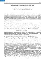
Proceedings of the 1st EPS/MetOp RAO Workshop, 15-17 May 2006, ESRIN, Frascati, Italy
(ESA SP-618, August 2006)

Knowledge Transfer: Heritage, in terms of knowledge
and technology, from I.P.F.’s experience in developing
and working with adapted sinusoidal grids should be
fully exploited.
3. DISCRETE GLOBAL GRIDS OVERVIEW
There are many different types of discrete global grids
each with different properties and therefore different
“best” uses, but as discussed in [1], global grids are
generally obtained by one of three main techniques:
Partitioning: The most commonly used regular DGGs;
the globe is partitioned along the geographic latitudelongitude
coordinate system. Its main advantage is that
historically the geographic coordinate system is a well
known and well used coordinate system and is the basis
for a varied number of datasets and processing software.
The two dimensional map of the geographic
projection is termed the Plate Carrée projection. Grids
based on square partitions are familiar and map effectively
to common data structures and display devices.
Raster data sets are often based upon cell regions with
edges defined by arcs of equal angle increments of
latitude and longitude (e.g. 0.5°×0.5°, 2.5°×2.5°).
Numerous adapted DGGs based upon the geographic
latitude-longitude grid have been implemented to address
some of the inherent limitations, such as strong
distortions at high latitudes. One such adaptation is to
decrease the number of cells with increasing latitude to
achieve more consistent cell size.
Tiling: With the application of more complex projection
systems the partitioning technique evolved into a
technique known as tiling. The globe, once in a specified
projection, is tiled with a square lattice which
forms a DGG. A map projection will either optimise
equal area, true shape or true distance or will provide a
compromise between them. For global remote sensing
applications the most important characteristic of a map
projection is that of equal area or equivalence. Therefore
area preserving projections such as the cylindrical
equal area projection are preferred.
Subdivision: In this case, the globe is inscribed into a
platonic solid whose faces are then subdivided into
regular shapes, such as triangles, diamonds or hexagons.
As noted by e.g. [2], there are only five so-called
platonic solids which can be used for this. Although
this method generates a DGG with uniform cell dimensions,
the cell dimensions cannot be chosen freely but
are determined by the particular geometrical division
used. The generation of such DGGs is complex, as is
the relationship between cell and geographic locations.
Whilst tiling or partitioning may be implemented on an
ellipsoid definition of the globe, most subdivision
techniques limit themselves to the sphere due to increased
complexity.
4. CANDIDATE GRIDS
In the following section four candidate DGG’s are
presented. The first two are current operational grids
used within I.P.F. The other two grids were selected as
one represents the most commonly used DGG for handling
of earth observation data (the EASE grid), and
the final DGG is selected as this is the pro-posed DGG
to be used for the future Soil Moisture and Ocean Salinity
(SMOS) mission.
4.1. The WARP4 Grid
The discrete global grid used in WARP version 4.0 for
ERS data aggregation is an adapted version of a sinusoidal
global grid applied on the sphere [3]. The grid is
generated in two steps.
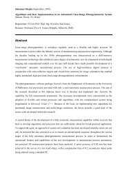
In the first step, a series of latitude small circles are
created, equally spaced with a central angle of 0.25º in
the south-north direction along any meridian, starting
with the south pole (Fig. 1). An Earth radius of
6370 km is assumed, yielding a constant spacing between
the latitude circles of
d = 6370 ⋅ 0.25 ⋅π
/180 ≈ 27.79 km , (1)
λ
suitable for the processing of 50 km resolution ERS
data [4].
In the second step, the Equator is also divided into
0.25º longitude intervals, giving 4·360=1440 divisions.
Each of the latitude circles created above is then subsequently
divided into 1440·cos(λ) divisions, where λ is
the latitude of the circle. This ensures the same
27.8 km spacing in the west-east direction as well,
subject to slight variations due to decimal rounding.
The number of grid points on each latitude circle decreases
thus with increasing latitude and thus addresses
high latitude distortion problems noted in [2]. The
WARP4 grid covers the land surface of the Earth with
more than 180000 single grid areas.
4.2. The QSCAT Grid
The so-called QSCAT grid is very similar to the
WARP4 grid described above and was implemented at
I.P.F. for storing and processing data from the Sea-
Winds scatterometer onboard the QuikSCAT platform
[5]. Unlike the WARP4 grid, it uses the Geodetic Reference
System 1980 (GRS 80) ellipsoid rather than the
sphere. Instead of using equal central angles between
the latitude circles, it uses an equal arc length of 10 km,
calculated as a local spherical (Gaussian) radius [6].
The longitudinal arc distances between grid points on
the same latitude circle are also set to 10 km, ensuring
consistent arc distances in the west-east direction at the
price of a discontinuity at the 180º meridian. Since this
region lies mostly in the Pacific Ocean, the discontinu-

ity does not influence retrieval of land parameters,
subject to a small area in the Russian far east.
4.3. The EASE Grid
The Equal-Area Scalable Earth Grid (EASE-Grid) was
created by the National Snow and Ice Data Center
(NSIDC), University of Colorado and the University of
Michigan Radiation Laboratory (RADLAB). It was
designed to suit the specific needs of SSM/I (Special
Sensor Microwave Imager) satellite data, but with a
potential for general application to any global scale
data set. In the EASE-grid, data can be expressed as
digital arrays of varying grid resolutions, defined in
relation to one of three possible projections, northern,
southern (both in Lambert’s Azimuthal Equal Area
projection) and global (in the Cylindrical Equal Area
projection). The grid is defined as a rectangular matrix
on each of the projections, where each column and row
can be easily matched to its latitude-longitude coordinate.
Row and column positions are computed differently
for each of the possible projections, thus marking
EASE as a non-global Earth grid. Another disadvantage
is its lack of uniform adjacency (due to the square
shape of its cells) and the distortions above mid latitudes
in the global projection [7]. Its main advantage is
the fact that square cells display very effectively on
digital output devices based on square lattices of pixels.
4.4. The SMOS Grid
The proposed grid recommended for implementation
for SMOS data was selected to fulfil two main requirements.
Firstly, it should maintain full information
content of the measured SMOS samples corresponding
to a maximum instrument resolution of 30 km. This
requirement translated to the necessity to select a uniformly
spaced global and isotropic grid at twice the
instrument resolution of 15km. Secondly, interpolation
error due to regridding to arbitrary user defined grids
should be minimised. This can be achieved by having a
uniform intercellular spacing. After a comparison of a
number of DGG’s, the Icosahedron Snyder Equal Area
(ISEA) Aperture 4 Hexagonal (ISEA4H) DGGS was
selected as the prime candidate [1]. The process of
a. b.
6. THE PROPOSED WARP5 GRID
Based on Tab. 1 we conclude that the most suitable
candidate grid, with the highest score, is the QSCAT
one. We therefore define the WARP5 grid as the
QSCAT grid, with the difference of using the GEM6
ellipsoid and a grid spacing arc length of a = 12.5 km.
The grid construction procedure described in Section
4.2 applied for WARP5 is illustrated in Fig. 1. The
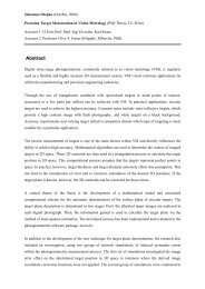
resulting grid configuration for three different areas is
shown in detail in Fig. 2, including the discontinuity at
the 180° meridian. For more accuracy, the radius of the
Earth used for calculating the latitude λ j of the latitude
small circles should be approximated with the radius of
curvature of the meridian, given in e.g. [6]. The discrete
longitudes along the latitude circles should be
calculated using the same Gaussian Earth radius apa
=
12.5 km
l j
a = 12.5 km
Figure 1. Constructing the WARP5 grid: a) equally
spaced latitude small circles; b) grid points created at
discrete longitudes on each latitude circle.
creating the grid involves subdividing the 20 equilateral
faces of the regular icosahedron into more triangles,
yielding 20 hexagons and 12 pentagons on the
surface of the sphere (the so-called resolution 1 grid).
Higher resolution grids (in discrete steps) are formed
by further tesselating the obtained shapes. Constructing
the higher-resolution ISEA grids requires usage of
complex forward and inverse projection formulas to
resolve cartesian to geographic coordinates as well as a
relatively advanced indexing system for the created
cells.
Table 1. Comparing the candidate grids.
Requirement WARP QSCAT EASE SMOS
Coverage
Equal Area
Geodetic
System
Grid Spacing
Data Access
Ease of im-
plementation
Score 4 5 3 3
5. ASSESMENT OF CANDIDATE GRIDS
As noted in [2], there is no single DGG that can provide
an optimum solution for all applications, and so in
the DGG assessment, as with any requirement driven
solution, the requirement criteria do have an order of
importance, and therefore a subjective weighting is
applied. In relation to the grid for the ASCAT soil
moisture products (hereafter termed the WARP5 grid)
is it critical that the requirements concerning efficient
data access, geodetic coordinate system, and ease of
implementation are fulfilled while keeping an as uniform
spacing of the grid cells as possible. The simple
compliance matrix in Tab. 1 presents a summary of the
assessment of the candidate grids.

0.50
-140
-160
-180
160
140
68
-120
120
-0.50 0
0.50
-100
-80
90
100
80
178 179 67.50 180 -179
-60
60
-0.50
-40
-20
89.50
0
20
40
67
a)
b)
c)
Figure 2. Details of three areas of the proposed grid: a) at its origin; b) at the North Pole; c) at the 180° meridian.
distance to nearest grid point (km)
12.500
12.490
12.480
12.470
12.460
12.450
0 10 20 30 40 50 60 70 80 90
latitude
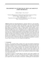
Figure 3. Nearest grid point distance and spanned
interlongitudinal angle.
proximation as for the QSCAT grid [6]. As a measure
of the grid spacing (where both the WARP4 and
QSCAT grids have been awarded negative marks in
Tab. 1), Fig. 3 shows the arc lengths between each grid
point and its closest neighbouring grid point (points
close to the discontinuity at the 180° meridian excluded).
It can be seen that that the arc length varies
reasonably from 12.455 km at the Equator to the nominal
12.500 km near to the poles. The diagram also
shows the increasing interlongitudinal distance between
grid points on different latitude circles expressed
as the longitudinal angle spanned by two neighbouring
points.
7. WARP5 GRID POINT INDEXING
Due to the large number of grid points (3264399 points
globally, distributed on 1601 latitude circles), the
WARP5 grid configuration would be practically incomplete
without fast and effective procedures for grid
point indexing and neighbourhood search. In our proposed
implementation we allow for regional processing
by organising the grid points into 20°×20° cells. We
also only consider grid points covering significant land
areas, using the land flags included in the scatterometer
1.8
1.5
1.2
0.9
0.6
0.3
interlongitudinal distance (degrees)
data or a static external land mask. We save all grid
point metadata (latitude, longitude, cell number, etc.) in
lookup tables in the form of arrays. Using the array
indices for the naming of the files holding the actual
backscatter time series for each grid point is an effective
way of accessing the data. For the quick resampling
of incoming data from orbit to grid geometry we
use neighbourhood search routines based on successive
geographic coordinate queries: for example, for an
incoming data frame of ASCAT measurements one
could first find a subset of grid points covering entirely
the extent of the data frame, followed by finding the
neighbourhoods of the individual frame data nodes
within the subset.
8. REFERENCES
1. Suess, M., et al., Processing of SMOS level 1c data
onto a discrete global grid. International Geoscience
and Remote Sensing Symposium
(IGARSS), Vol. 3, 1914–1917, 2004.
2. Sahr, K., et al., Geodesic discrete global grid systems.
Cartography and Geographic Information
Science, Vol. 30(2), 121–134, 2003.
3. Wagner, W., Soil Moisture Retrieval from ERS
Scatterometer Data, dissertation, Vienna University
of Technology, Vienna, Austria, 1998.
4. Scipal, K., Global Soil Moisture Retrieval from ERS
Scatterometer Data, dissertation, Institute of Photogrammetry
and Remote Sensing, Vienna University
of Technology, Vienna, Austria, 2002.
5. Kidd, R. A., et al., The development of a processing
environment for time-series analysis of SeaWinds
scatterometer data. International Geoscience and
Remote Sensing Symposium (IGARSS), Vol. 6,
4110–4112, 2003.
6. Torge, W., Geodesy, 3rd Edition, , Chapter 4.1: The
Rotational Ellipsoid. de Gruyter, 2001, ISBN: 3-
11-017072-8.
7. Brodzik, M., J., EASE-Grid: A Versatile Set of
Equal-Area Projections and Grids, http://nsidc.org/
data/ease/ease_grid.html, web resource accessed
on 1 Aug. 2005.