measurement eccentricties of circular targets in vision metrology

MEASUREMENT ECCENTRICTIES OF CIRCULAR TARGETS IN
VISION METROLOGY
Johannes Otepka a , Clive S. Fraser b
a Institute of Photogrammetry & Remote Sensing, Technical University of Vienna,
Gusshausstrasse 27-29/E122, 1040 Vienna, Austria
Email: jo@ipf.tuwien.ac.at
b Department of Geomatics, University of Melbourne, Victoria 3010, Australia
Email: c.fraser@unimelb.edu.au
Abstract: In digital close-range photogrammetry, commonly referred to as vision metrology,
circular targets are often used for high precision applications. The most common target type
used consists of retro-reflective material, which provides a high contrast image with flash
photography. The measurement of image coordinates of signalised targets continues to be a
factor limiting the achievable accuracy of high-precision vision metrology systems.
Mathematical algorithms are used to determine the centres of imaged targets in 2D space.
These 2D centroids are then used in a triangulation process to calculate the target position in
3D space. This computational process assumes that the targets represent perfect ‘points’ in
space. However, in practice target-thickness and target-diameter can adversely effect this
assumption, leading to the introduction of systematic errors and to incorrect calculation of 3D
position. The paper presents mathematical formulae which rigorously describe these errors
and allow the computation of corrections for the triangulation process. Moreover, the
distortion effect of the eccentricities is analysed for different network simulations, as well as
for a real test field. It will be shown that these measurement eccentricities can lead to
incorrect object coordinates in the case of high precision applications.
1. Introduction
Nowadays, vision metrology (VM) is regularly used in large-scale industrial manufacturing
and precision engineering. VM strategies employ triangulation to determine 3D object point
coordinates. To achieve accuracy to 1 part in 100,000 and better, special targets are used to
mark points of interest. Various investigations have shown that circular targets deliver the
most satisfactory results regarding accuracy and automated centroid recognition and
mensuration. For such targets, retro-reflective material is widely used because on-axis
illumination of these targets returns many times more light than a normal textured surface.
This results in high contrast images, which are a key requirement for high precision in digital
close-range photogrammetry.
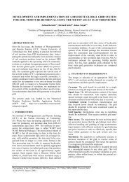
The perspective properties of circular targets are such that a circle which is parallel to the
image plane will appear as a circle. In all other cases the circular target will project as an
ellipse or in general as a conic section, as indicated in Figure 1. Parabolic and hyperbolic
curves appear only if the circle touches or intersects the “vanishing plane” (the plane parallel

to the image plane, which includes the projection centre). Because of the typically small size
of targets employed and the limited field of view of the measuring devices, it is unlikely that
these circular targets will appear as parabolic or hyperbolic curves. Therefore, only elliptical
images are considered in the following.
Figure 1: Perspective view of circle
VM systems use centroiding algorithms to compute the centres of each ellipse, these centroids
becoming the actual observations for the triangulation process. However, it is well known that
the centre of a circle does not project onto the centre of the ellipse, which thus introduces a
systematic error in any triangulation process. There are two reasons why this error is
universally ignored in today’s VM systems. First, the effect is small, especially in the case of
small targets (e.g. [2] and [3]). Second, prior to the method developed by the first author [7],
there had been no practical approach to automatically determining the target plane, which is a
basic requirement for the correction of this error.
This paper presents the rigorous mathematical connection between a circular target and its
perspective image. The derived formulae can be employed both to determine the plane of the
circular targets and to compensate image observations (which are the ellipse centres) for the
above mentioned eccentricity. Additionally, the distortion effect of the eccentricity will be
analysed for different networks configurations. Moreover, experimental results will be
presented, where the object point coordinates are distorted to a magnitude well exceeding the
measurement precision if the eccentricities are ignored within the bundle adjustment.
The derived formulae have been implemented and evaluated in Australis, a photogrammetric
software package for off-line VM (compare [4] and [8]). Hence, Australis is the ideal tool to
analyse the distortion effect of the eccentricity since the software is capable of determining
the target plane information and compensating for it within the triangulation process.
2. Mathematical Connection of a Circular Target and its Perspective Image
In [1] a solution is given to calculate and correct the eccentricity if the elements of the target
circle are given. This mathematical model describes the relationship between the ellipse
centre and the circle parameters, considering a certain target-image configuration. In a
previously derived solution by Kager [5], it was demonstrated how to calculate a 3D circle
from a given imaged ellipse by analysing resulting quadratic matrices. However, both
solutions are unable to describe the parameters of the imaged conic section explicitly by the
circle elements as derived in this section. Such formulae allow the derivation of an adjustment
model of indirect observations using multiple images to determine the corresponding circular
target in space.

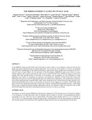
As illustrated in Figure 2, a cone is given which touches the circular target and the apex of the
cone is positioned at the projection centre C of the image. Then the cone is intersected with
the image plane. If the resulting section figure can be put into the same mathematical form as
an implicit ellipse equation (general polynomial of second degree) the problem is solved.
Figure 2: View cone which touches the circular target
In object space, the circular target can be described as
P= M+ r ⋅(cosα⋅ e1
+ sinα⋅e 2 )
(1)
where M is the centre of the circle, r defines the circle radius, e 1 and e 2 are arbitrary
orthogonal unit vectors within the circle plane and α is the circle parameter. Based on
equation (1) the cone of Figure 2 is given by
( )
X= C+ λ⋅r
⋅ cosα⋅ e + sin α⋅ e + λ⋅( M−C )
(2)
1 2
where α and λ are the cone parameters. To transform the cone into image space the wellknown
collinearity condition is used.
⎛ x ⎞ ⎛R1⎞ ⎛R11 R12 R13⎞ ⎛ Xx
− C
⎜ ⎟ ⎜ ⎟ ⎜ ⎟ ⎜
x= y = R⋅ X− C = R ⋅ X− C = R R R ⋅ X −C
( ) ( )
2
21 22 23
⎜ c⎟ ⎜ ⎟ ⎜
3
R31 R ⎟ ⎜
⎝−
⎠ ⎝R
⎠ ⎝ 32 33⎠ ⎝
R X −C
where x and y are the images coordinates, c is the focal length, R is the rotation matrix and X
are coordinates in object space. Hence, the cone in image space follows as
( )
x= λ⋅r
⋅R⋅ cosα⋅ e + sin α⋅ e + λ⋅R⋅( M −C)
(4)
1 2
The intersection of equation (4) with the image plane is determined in a simple manner. The
plane is defined by z = -c. Thus, λ can be described by
c
λ =−
R ⋅( r⋅cosα⋅ e + r⋅sin α⋅ e + M−C)
3
1 2
and the coordinates of the intersection figure follow as
R1 ⋅( r⋅cosα
⋅ e1 + r⋅sin α ⋅ e2
+ M −C)
R1
⋅g
x =− c =−c
R ⋅( r⋅cosα
⋅ e + r⋅sin α ⋅ e + M −C)
R ⋅g
3 1 2
3
R2 ⋅( r⋅cosα
⋅ e1 + r⋅sin α ⋅ e2
+ M −C)
R2
⋅g
y =− c =−c
R ⋅( r⋅cosα
⋅ e + r⋅sin α ⋅ e + M −C)
R ⋅g
3 1 2
3
y
z
x
y
z
⎞
⎟
⎟
⎠
(3)
(5)
(6)

If the equations (6) can be transformed so that the parameter α is eliminated, the problem is
solved. First, the equations are transformed as shown below:
−R3⋅g ⋅ x = c⋅R1⋅g
⇒
−R ⋅g ⋅ y = c⋅R ⋅g
3 2
( 1 1) α( 2 2)
( ) α( )
rcosα
−x⋅R ⋅e −c⋅R ⋅ e + rsin −x⋅R ⋅e −c⋅R ⋅e = ( x⋅ R + c⋅R ) ⋅( M−C)
3 1 3 1 3 1
rcosα
−y⋅R ⋅e −c⋅R ⋅ e + rsin −y⋅R ⋅e −c⋅R ⋅e = ( y⋅ R + c⋅R ) ⋅( M−C)
Equation (8) can also be described as
3 1 2 1 3 2 2 2
3 2
rcosα⋅ x1+ rsinα⋅y1 = c1 ⋅x2
⎫⎪ ⋅− y2⎫
⎬+ ⎬ +
(9)
rcosα⋅ x2 + rsinα⋅y2= c2 ⋅−x1⎪⎭
⋅y1
⎭
or, after the proposed transformations, the following two equations are generated:
( )
( )
rsinα
y x y x c x c x
2
1 2− 2 1
=
1 2− 2 1 ⎫
2 ⎬ +
1 2 2 1 2 1 2 2
rcosα
y x − y x = c y −c y ⎭
After squaring and adding equations (10) the final sought-after equation without an α term is
found:
2 2
( ) ( ) (
2
r y1x2 y2x1 c1x2 c2x1 c2y1 c2y2
(7)
(8)
(10)
− = − + − ) 2 (11)
This equation can be transformed into a general polynomial of the second degree in x and y as
a ⋅ x + a ⋅ xy+ a ⋅ y + a ⋅ x+ a ⋅y− = (12)
2 2
1 2 3 4 5
1 0
where the corresponding coefficients are
r ⋅i − j −k
a1
=
d
2 2 2 2
1 1 1
2
r ⋅i1⋅i2 − j1⋅ j2 −k1⋅k2
a2
= 2
d
2 2 2 2
r ⋅i2 − j2 −k2
a3
=
d
2
j1⋅ j3 + k1⋅k3−r ⋅i1⋅i3
a4
= 2⋅c
d
2
j2⋅ j3 + k2⋅k3−r ⋅i2⋅i3
a5
= 2⋅c
d
using the following auxiliary variables
( 3 3 3 )
d c j k r i
2 2 2 2 2
= + − ⋅ (14)
T
( i i i ) ( ) ( ) ( )
i = = R⋅ e × R⋅ e = R⋅ e × e = R⋅n
1 2 3 1
1 2 3 1 ( ) ( 1 ( )) ( 1×
)
T
( k1 k2 k ) ( 2) ( ( )) ( 2 ( )) ( 2×
)
T
( j j j ) ( ) ( )
j = = R⋅ e × R⋅ C− M = R⋅ e × C− M = R⋅
e v
k = = R⋅ e × R⋅ C− M = R⋅ e × C− M = R⋅
e v
3
2 1 2
(13)
(15)

It is permitted to use the distributive law in equations (15) since R is a rotation matrix.
Equations (12) to (15) explicitly describe the parameters of the imaged conic section via the
circle elements. Although the general problem is solved, additional simplifications can be
applied. In the following derivations, an interesting invariance of orthogonal unit vectors
appears.
While infinite sets of the vectors e 1 and e 2 exist to describe the same circle in space, the
polynomial coefficients (13) have to be invariant regarding the selected vector set. Since the
normal vector of the circle plane (n in object space; i in image space) is invariant to e 1 and e 2
as well, it has to be possible to find a description of equations (13) using only the vectors i
and v (= C - M). It is noticeable that the elements of the vectors j and k always appear
combined and in quadratic form within the coefficients. If these 6 quadratic sums can be
expressed by i and v, the problem is solved.
For the following derivation the unit vectors e 1 and e 2 in image space are defined by using
rotation matrices as
e1
e
2
⎛1⎞ ⎛ cosβ
cosγ
⎞
= RXαRYβRZγ
⋅
⎜
0
⎟ ⎜
sinα sinβ cosγ cosα sinγ
⎟
= −
⎜0⎟ ⎜cosα sinβ cos γ+ sinα sinγ
⎟
⎝ ⎠ ⎝ ⎠
⎛1⎞ ⎛ −cosβ
sinγ
⎞
= RXαRYβRZ
π
⋅
⎜
0
⎟ ⎜
sinα sinβ sinγ cosα cosγ
⎟
γ +
= − −
2 ⎜0⎟ ⎜−cosα sinβ sin γ+ sinα cosγ
⎟
⎝ ⎠ ⎝ ⎠
where γ describes the degrees of freedom within the circle plane and RX, RY and RZ are
rotation matrices defined by
⎛1 0 0 ⎞ ⎛cosβ 0 −sinβ⎞ ⎛ cosγ sinγ
0⎞
RX =
⎜
0 cosα sinα ⎟ ⎜
0 1 0
⎟ ⎜
sinγ cosγ
0
α RY =
β RZ = −
⎟
γ
⎜0 −sinα cosα⎟ ⎜sin β 0 cos β ⎟ ⎜
⎝ ⎠ ⎝ ⎠ ⎝ 0 0 1⎟
⎠
Substituting vectors e and e in equations (15) it follows that
1 2
(16)
(17)
⎛ sin β ⎞
i = e
⎜
1× e = −sinα
cos β
⎟
2
⎟
⎜−cosα
cos β
⎝
⎠
( )
j= e × R⋅ v = e × v =
1 1
( sinα sin β cosγ − cosα sinγ ) + v ( −cosα sin β cosγ −sinα sinγ
)
v1( cosα sin β cosγ sinα sinγ ) v3cos β cosγ
v ( − sinα sin β cosγ + cosα sinγ ) + v cos β cosγ
⎛v3 2
⎜
= ⎜
+ −
⎜
⎝
( )
k = e × R⋅ v = e × v =
2 2
1 2
( −sinα sin β sinγ − cosα cosγ ) + v ( cosα sin β sinγ −sinα cosγ
)
v1( cosα sin β sinγ sinα cosγ ) v3cos β sinγ
v ( sinα sin β sinγ + cosα cosγ ) −v
cos β sinγ
⎛v3 2
⎜
= ⎜
− + +
⎜
⎝
1 3
⎞
⎟
⎟
⎟
⎠
⎞
⎟
⎟
⎟
⎠
(18)
(19)
(20)

where it can be seen that the normal vector i does not depend on γ. However, the vectors j and
k still contain γ terms. The next step is to compute the aforementioned quadratic sums using
equations (19) and (20). As an example, the following sum will be fully derived.
( )
2 2
2
2 2 2
2
2 2 2
1 1 3
sin β cos α cos β
2
(1 cos α cos β) 2
3 2cosαsin α cos
j + k = v + + v − + v v
β (21)
As expected all γ terms are eliminated. Now, the angle terms can be substituted by the
elements of the vector i (18) which results in
2
( ) (1 ) 2 ( ) ( )
2 2
2
2 2
2
2 2
2
1 1 3 1 3 2 3 3 2 2 3 2 2 3 3 1 2 3
j + k = v i + i + v − i + v v i i = v i + v i + i v + v
2 (22)
considering that i is a unit vector. This substitution can also be carried out for the other five
remaining quadratic sums. The final results are listed below.
2 2 2
( )
2 2 2
( )
( )( )
2
( 1) ( )
( )( )
j + k =− vi − v i + v + v
2 2
2 2 1 3 3 1 1 3
j + k = − v i − vi + v + v
2 2
3 3 2 1 1 2 1 2
j j + kk = vi −vi vi −vi −vv
1 2 1 2 3 1 1 3 3 2 2 3 1 2
jj+ kk = vv i − + v − vii+ vii−vii
1 3 1 3 1 3 2 2 1 2 3 2 1 3 3 1 2
j j + k k = vi −v i vi −v i −v v
2 3 2 3 1 3 3 1 1 2 2 1 2 3
Using equation (23) the polynomial coefficients (13) can be finally described using r, c, i and
v as parameters only.
2
3
4
5
= 2
2 2 2
( ) ( )
r ⋅i − v i + v i − i v + v
a1
=
d
a
a
a
a
where d is
2 2 2
1 2 2 3 3 1 2 3
( )( )
2
r ⋅i1⋅i2 − v3i1−vi 1 3
v3i2 − v2i3 + v1v2
( )
2
2 2
2 2
⋅
2
+
1 3− 3 1
−
1
−
3
r i vi v i v v
=
d
( 1) ( )
vv i − + v − vii + vii −vii −r ⋅i⋅i
= 2 ⋅c
d
= 2 ⋅c
d
2 2
1 3 2 2 123 213 312 1 3
( )( )
vi −vi vi −vi −v v −r ⋅i ⋅i
2
13 31 12 21 2 3 2 3
2 2 2
2 2
( ( 21 12)
1 2 3 )
2
d = c − v i − vi + v + v −r ⋅i
d
Equations (24) and (25) not only describe the connection between a circular target and its
perspective image, but also these equations, considering mathematical rigorousness, represent
new observations equations for the bundle adjustment. In this model each image point
consists of 5 observations and any object point will be characterised by 7 unknowns (centre
point M, target normal n and radius r). In consequence the matrices of the bundle adjustment
would increase dramatically. This can be avoided if the equation system is solved iteratively:
(23)
(24)
(25)

1. Perform standard bundle adjustment;
2. Employ equations (24) and (25) to adjust the target elements (M, n and r) of all object
points considering the exterior orientation (EO) of all images and the camera calibration
as fixed;
3. Compute bundle adjustment using image coordinate observations which are
compensated for the eccentricity; and
4. Go back to 2 until convergence.
One iteration is usually enough to achieve convergence for standard VM applications.
In comparison to the standard utilisation process, the described strategy requires full ellipse
information of each imaged target. Though the extraction of the target centre is well known in
Computer Vision, the determination of the full ellipse information is a delicate problem since
targets are typically only a few pixels in diameter. Appropriate computation algorithms,
considering the special circumstantiates of VM, are described in [6] and [7]. Finally it should
be noted that the derived formulae are equivalent to the solutions presented in [1] and [5].
3. The Distortion Effect of Eccentricities within the Bundle Adjustment
Earlier investigations ([2] and [3]) have studied the impact of the eccentricity error within a
bundle adjustment. It was reported that in a free network adjustment with or without
simultaneous camera calibration, the eccentricity error caused by moderately sized image
targets is almost fully compensated for by changes in the exterior orientation parameters (and
the principal distance) without affecting the other estimated parameters.
Network simulations performed by the authors have shown good agreement with earlier
findings, especially when employing test fields with little variation in the target normals.
However, test fields with a significant range of target orientations and with medium to large
sized targets can show significant distortions within the triangulated object point coordinates,
as shown in the following (distortion of the EO and the camera calibration parameters are not
considered since they are irrelevant for standard VM applications)
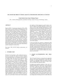
The first test field describes the surface of a parabolic antenna with a diameter of 1.4 m
(Figure 3). In contrast to the relatively low target orientation variation of the parabolic surface
a second sinus-shaped surface (horizontal extent of 3 by 5 m) was chosen, as indicated in
Figure 4. For both surfaces, 16 artificially generated images were computed using a typical
VM camera (c of 20 mm, resolution of 1500 by 1000 pixels). The target size was selected
such that the resulting average target diameter within the images was nearly the same for both
networks, namely ~19 pixels.
To investigate the eccentricity error, a free network adjustment using intensity-weighted
target centroids was performed. Afterwards, the computed object coordinates were
transformed into the original (error-free) coordinate reference frame. The resulting positional
discrepancies are illustrated in Figure 5 and listed in Table 1.
Expected accuracy
(triangulation precision
Discrepancies
(transformation)
Object point sigma
(bundle adjustment)
1:100 000) Mean Max Mean Max
Parabolic antenna 0.014 0.012 0.020 0.001 0.001
Sinus-shaped Surface 0.050 0.080 0.123 0.011 0.016
Table 1: Results of simulated networks (all values in mm)

Figure 3: Parabolic antenna surface (d =1.4 m) Figure 4: Sinus-shaped surface (3 x 5 m)
From the results, interesting conclusions can be drawn. First, the eccentricity error can
systematically distort the object point coordinates, this being visible in Figure 5. The use of
high quality digital equipment allows the achievement of typical triangulation accuracies of
1:100,000, which is about 0.014 and 0.05 mm in these cases. The object point sigmas
obtained from the bundle adjustment (right column of Table 1) are well within the expected
accuracy. (The sigmas only reflect the eccentricity effect since the observations were
simulated). However, the real accuracy of the object point coordinates is visible in the column
of transformation discrepancies (column with grey background of Table 1). Compared to the
expected triangulation precision, the distortion effect of the eccentricity is higher for the
sinus-shaped surface than for the parabolic antenna. This is caused by the higher variation in
target orientation. Summarizing, it can be said that, for certain configurations, the amount of
distortion can clearly exceed the measurement accuracy of VM.
Figure 5: Discrepancy vectors between adjusted object coordinates and original coordinates
Finally, a ‘dangerous’ effect for practical applications can also be observed. Since the
adjustment parameters compensate for the eccentricity error, the bundle adjustment estimates
the accuracy of the object coordinates too optimistically (up to factor 10 in these cases),
which may lead to misinterpretation, eg in deformation measurements. Consequently, it was
necessary to ‘design’ a special network configuration to reveal the eccentricity effect within a
real test field, as presented in the following section.

4. Evaluation of the Simulation Results within a Real Test Field
In simulated networks it is easy to obtain the eccentricity distortion of the object coordinates
since the ‘error-free’ coordinate reference frame is known. For a real test field the situation is
quite different. The previous strategy can be applied only if ultra-precise coordinates of the
targets are given. Since the magnitude of the resulting errors is only about 0.01 mm (in case
of a 1 m test field), the required precision for the reference coordinates is very difficult to
achieve. Hence, a different strategy was used to examine the eccentricity distortion.
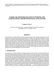
A plane test field consisting of 27 retro-reflective targets using a special scale bar was
employed. The field was surveyed three times moving the scale bar into three different
positions between each survey, as indicated in Figure 6. Whereas scale bar position one and
two were roughly within the test field plane, scale bar position three was slanted with an angle
of about 30°. A comparison of the three scale bar distances derived from the adjusted object
coordinates should then reveal the eccentricity effect.
The scale bar had a length of about 0.5 m and consisted of 2 targets which enclosed an angle
of about 30°, as shown in Figure 7. Different target orientations cause different distortion
vectors which is absolutely necessary for this distance comparison method. To achieve
distinguishable distance differences, large targets (average target diameter to ~50 pixels) were
employed for the scale bar.
Target normal
~ 30°
Target
Figure 6: Test field (1.5 x 1.5 m) with scale
bar in three different positions.
Figure 7: Special arrangement of targets on
the scale bar.
A total of 54 images (3 x 18 images) were recorded using a GSI Inca camera (resolution of
2029 by 2048 pixels, 18 mm lens), and the network was processed twice, using the standard
bundle adjustment and then the modified adjustment with applied eccentricity corrections.
The resulting distances computed from the object coordinates of the two adjustments are
given in Table 2. In the case of uncorrected observations the maximum distance difference
(grey background column) is four times larger than would be expected from the object point
sigmas. If the eccentricity corrections are applied, on the other hand, the maximum distance
error is well within the object point accuracy. The identical object point sigmas support the
previous statement that the distortional effect of the eccentricity is not visible within sigmas
obtained from the bundle adjustment.
Dist. 1 Dist. 2 Dist. 3
Max. dist. Object point sigma
difference (bundle adjustment)
Results without corr. 437.172 437.143 437.089 0.083 0.018
Results with corr. 437.256 437.242 437.245 0.014 0.018
Table 2: Bundle adjustment results with and without eccentricity corrections (values in mm).

One could argue that these results have no relevance for practical applications since such
large targets were employed. However, the results only identify relative distortions.
Considering the object coordinates obtained from the ‘corrected’ adjustment as error-free
compared to the uncorrected case, a similar analysis as made for the simulated network can be
performed. It turns out that the average discrepancy of the scale bar points exceeds 0.3 mm.
This is 17 times larger than the object point sigma (note that sigma naught was identical for
both bundle adjustments). It can be concluded that even clearly smaller targets will be
distorted above the measurement precision as derived in the network simulations.
5. Conclusion
In the first part of the paper, rigorous formulae were presented which describe the connection
of a circular target and its perspective image. Utilizing these equations the target plane can be
determined and the eccentricity of the image observations can be compensated. Additionally
it has been shown that the eccentricity can cause object coordinate distortions which are well
above the measurement variance in the case of high precision applications. In standard VM
software the only way to avoid eccentricity distortion is to keep the targets as small as
possible (target diameter should not exceed 5 pixels). However, this cannot be achieved in
general since there will always be different scales in different parts of the images. Therefore,
the authors propose adoption of the automatic eccentricity correction processes, as
implemented in Australis. This will remove target size limitations caused by the eccentricity,
which will in turn lead to even higher achievable measurement precision in VM.
Acknowledgement
Many thanks to Danny Brizzi of Vision Metrology Services of Melbourne, for imaging the
scale bar test field as described in Section 4.
References:
[1] Ahn, S.J., Warnecke, H.-J. and Kotowski, R.: Systematic Geometric Image
Measurement Errors of Circular Object Targets: Mathematical Formulation and
Correction, Photogrammetric Record, 16(93), 485-502, 1999.
[2] Ahn, S. J. and Kotowski, R.: Geometric image measurement errors of circular object
targets. Optical 3-D Measurement Techniques IV (Eds. A. Gruen and H. Kahmen).
Herbert Wichmann Verlag, Heidelberg. 494 pages: 463–471, 1997.
[3] Dold, J.: Influence of large targets on the results of photogrammetric bundle adjustment.
International Archives of Photogrammetry & Remote Sensing, 31(B5): 119–123, 1996.
[4] Fraser, C. S. and Edmundson, K .L.: Design and implementation of a computational
processing system for off-line digital close range photogrammetry. ISPRS Journal of
Photogrammetry and Remote Sensing, 55(1): 94-104, 2000.
[5] Kager H.: Bündeltriangulation mit indirekt beobachteten Kreiszentren.
Geowissenschaftliche Mittelungen Heft 19, Institut für Photogrammetrie der
Technischen Universität Wien, 1981.
[6] Otepka, J., Fraser, C.S.: Accuracy Enhancement of Vision Metrology through
Automatic Target Plane Determination, Proceedings of the ISPRS Congress, 2004.
[7] Otepka J.: Precision Target Mensuration in Vision Metrology, PHD Thesis, Vienna
University of Technology, 2004.
[8] Photometrix, Web site: http://www.photometrix.com.au (accessed 6 June 2005).