Poland - IOW

Input and fate of dissolved nitrogen compounds via
submarine groundwater discharge into the Puck Bay
(Poland)
Diplomarbeit
am
Leibniz Institut für Ostseeforschung Warnemünde (IOW)
an der
Universität Rostock
vorgelegt von
Sabine Nestler
Rostock, Mai 2011
Gutachter:
Dr. habil. Maren Voß
Dr. habil. Stefan Forster

Abbreviations
I
Abbreviations
BC benthic chamber
C carbon
DIN dissolved inorganic nitrogen
DON dissolved organic nitrogen
IN inorganic nitrogen
L groundwater lance
N nitrogen
+
NH 4
-
NO 3
-
NO 3
ammonium
nitrate
nitrite
NO - 2/3 sum of NO - -
3 and NO 2
POM particulate organic matter
SGD submarine groundwater discharge
O 2
OM
T
oxygen
organic matter
push pull lance
TDN total dissolved nitrogen

Abstract
II
Abstract
The aim of this study was the investigation of nitrogen input to the Puck Bay (Poland) via
submarine groundwater discharge (SGD) and its ecological impact. Thus concentrations of
dissolved organic nitrogen (DON), nitrate, nitrite and ammonium were measured in pore
waters of SGD impacted and unimpacted sites at Hel Penisula (Poland). Furthermore the
δ 15 N-NH 4 + values as well as the δ 15 N and δ 13 C values of various organisms were determined.
Nitrate and nitrate were nonexistent in the discharging groundwater and DON of pore water
showed concentrations about 20 µmol L -1 , similar to the water column concentrations, but
could not be associated with SGD. The dominant nitrogen species in the SGD was by far
ammonium with concentrations ranging from 200 to 5000 µmol L -1 . This high range in
concentrations also indicates the variability of nitrogen input in time and space.
In order to identify the source of the ammonium in the SGD a deep and a shallow well were
sampled on Hel Peninsula. Since both these wells contained only relatively low ammonium
concentrations about 30 µmol L -1 the corresponding aquifers can not be the source of the high
ammonium load of the SGD. It was therefore hypothesized that the ammonium may originate
from organic rich sediment layers overlying a deep aquifer and that the ammonium is
dissolved in groundwater from a deep aquifer seeping upwards through this layer prior to
submarine discharge. The relatively low δ 15 N-NH 4 + values between 0 and 2 ‰ support such a
hypothesis indicating a terrigenous source of nitrogen like degradation of soil organic matter.
The high ammonium load of the SGD would therefore not be of anthropogenic origin.
Ammonium from SGD was mostly conservatively mixed into the water column without any
significant transformation. Extrapolations from ammonium flux rates of the SGD to the whole
Puck Bay indicate a high overall nitrogen load from SGD compared to other nitrogen sources.
However, the ammonium load from SGD did not seem to have a significant impact on the
Puck Bay ecosystem since organisms sampled on the SGD impacted site showed the same
δ 15 N values as organisms sampled from the SGD unimpacted Baltic Sea side and the two food
webs looked quite similar.
Finally, to exactly understand the sources and sinks of ammonium from SGD on Hel Penisula
and its ecological significance further investigations of the hydrogeological conditions and the
ecosystem of the Puck Bay are necessary.

Abstract
III
Zusammenfassung
Das Ziel dieser Arbeit war es den Stickstoffeintrag und damit den ökologischen Einfluss
durch submarine Grundwasseraustritte (SGD) in die Puck Bay (Polen) zu untersuchen. Dafür
wurden die Konzentrationen von organischem gelösten Stickstoff (DON), Nitrat, Nitrit und
Ammonium im Porenwasser gemessen, sowohl in Grundwasser beeinflussten als auch in
unbeinflussten Gebieten auf der Halbinsel Hel. Außerdem wurden die δ 15 N Werte im
Ammonium sowie die δ 15 N und δ 13 C Werte von verschiedenen Biota bestimmt. Nitrat und
Nitrit kamen nicht im austretenden Grundwasser vor. DON Konzentrationen von ca. 20 µmol
L -1 im Porenwasser waren ähnlich den Konzentrationen, die in der Wassersäule gemessen
wurden und konnten nicht mit den submarinen Grundwasseraustritten in Verbindung gebracht
werden. Die Stickstoffspezies, die mit Abstand in den höchsten Konzentrationen von 200 bis
5000 µmol L -1 im Grundwasser auftrat war Ammonium. Die große Spanne in den
Ammoniumkonzentrationen zeigte auch die große räumliche und zeitliche Variabilität.
Um die Quelle des Ammoniums aus den submarinen Grundwasseraustritten ausfindig zu
machen wurden ein tiefer und ein flache Brunnen auf Hel beprobt. Da allerdings die
Grundwässer beider Brunnen nur relative geringe Ammoniumkonzentrationen von ca. 30
µmol L -1 enthielten, können die beiden entsprechenden Grundwasserleiter nicht die Quelle für
die große Ammoniumfracht sein, die in den Grundwasseraustritten gefunden wurde. Auf
Grund dessen wurde die Hypothese aufgestellt, dass das Ammonium aus Organik reichen
Schichten stammt, die über einem tiefen Grundwasserleiter liegen. Danach wird das
Ammonium im Grundwasser gelöst bevor es in die Puck Bay austritt, während dieses durch
eben diese Schichten aufsteigt. Die relativ niedrigen δ 15 N Werte im Ammonium zwischen 0
und 2 ‰ sprechen für diese Hypothese, da sie auf eine terrigene Stickstoffquelle wie den
Abbau von organischem Material im Boden hindeuten. Demnach wäre das Ammonium aus
den submarinen Grundwasseraustritten nicht anthropogenen Ursprungs.
Das austretende Ammonium wurde hauptsächlich konservativ in die Wassersäule eingemischt
ohne vorherige Umwandlung. Extrapolationen von Ammoniumflussraten der
Grundwasseraustritte auf die ganze Puck Bucht deuten auf eine hohe Stickstofffracht hin
verglichen mit anderen Quellen. Allerdings scheint das Ammonium keinen deutliche Einfluss
auf das Ökosystem der Bucht zu haben, da die Organismen, die im Grundwasser beeinflussten
Gebiet gesammelt wurden, die selben Isotopenwerte Werte zeigten, wie Organismen von der
Ostseeseite der Halbinsel Hel ohne SGD.

Abstract
IV
Um die Quellen und Senken für das Ammonium aus dem Grundwasser richtig zu verstehen
und damit auch seine ökologische Bedeutung für die Puck Bucht sind weitere
Untersuchungen der hydrogeologischen Bedingungen und des gesamten Ökosystems nötig.

Table of Contents
V
Table of Contents
Abbreviations.............................................................................................................................I
Abstract.................................................................................................................................... II
Table of Contents .................................................................................................................... V
1 Introduction ...................................................................................................................... 1
2 Material and Methods...................................................................................................... 6
2.1 Sampling Site......................................................................................................................... 6
2.2 Sampling ................................................................................................................................9
2.3 Laboratory experiment with artificial sediment cores ......................................................... 14
2.4 Analytical methods .............................................................................................................. 17
2.4.1 Determination of DIN ................................................................................................................... 17
2.4.2 Determination of DON.................................................................................................................. 18
2.4.3 Stable Isotopes .............................................................................................................................. 18
2.5 Mass spectrometric analyses................................................................................................ 19
2.6 End-member mixing calculations ........................................................................................ 20
3 Results ............................................................................................................................. 22
3.1 Seasonal and temporal variability........................................................................................ 22
3.2 Spatial variability................................................................................................................. 26
3.3 δ 15 N values of ammonium ................................................................................................... 31
3.4 Comparison of SGD influenced sites with a Baltic Sea station ........................................... 36
3.5 Benthic Chambers................................................................................................................ 37
3.6 Core incubation experiment in the laboratory...................................................................... 39
3.7 Isotope values in biota ......................................................................................................... 40
4 Discussion........................................................................................................................ 45
4.1 SGD and its nitrogen load.................................................................................................... 45
4.1.1 Spatial distribution of SGD........................................................................................................... 45
4.1.2 Temporal variability of SGD......................................................................................................... 47
4.1.3 Extrapolating exercise for SGD .................................................................................................... 48
4.1.4 DON in the SGD ........................................................................................................................... 49
4.1.5 DIN in the SGD............................................................................................................................. 50
4.1.6 Seasonality of ammonium from SGD ........................................................................................... 51
4.1.7 Spatial variability of ammonium from SGD ................................................................................. 52
4.1.8 Estimate of ammonium input to the Puck Bay via SGD ............................................................... 54
4.2 Source identification ............................................................................................................ 55
4.2.1 Sources of the SGD....................................................................................................................... 55
4.2.2 Sources of ammonium from SGD................................................................................................. 56
4.3 Reactions within the sediment ............................................................................................. 60
4.4 Reactions after release to water ........................................................................................... 61
4.5 Conclusion ........................................................................................................................... 63
5 Bibliography ................................................................................................................... 64
Danksagung............................................................................................................................. 72
Selbständigkeitserklärung:.................................................................................................... 73

Introduction 1
1 Introduction
Eutrophication of coastal waters due to nonpoint source land-derived nitrogen (N) loads is
perhaps the greatest agent of change altering coastal ecology (National Research Council,
2000). Global river-derived nutrient inputs into the ocean have tripled since the 1970’s (S. V.
Smith et al., 2003). However, little is known how much of this originates from groundwater
input into rivers and estuaries. Submarine groundwater discharge (SGD) to the coastal ocean
is a worldwide phenomenon. But since it occurs mostly only in a diffusive and temporal and
spatial very heterogeneous way, localization and quantification is difficult. Hence SGD and
its impact on geochemical cycling in the coastal ocean have been neglected for a long time. In
addition groundwater flow is much slower than riverine flow and therefore the volume
discharged is lower. Most estimates of terrestrially derived SGD range from 6 to 10 % of
surface water inputs (Burnett et al., 2003).
However, the exchange of groundwater between land and sea is a major component of the
hydrological cycle (Moore, 2010). Groundwater may be a major route of transport from land
to sea for freshwater and associated land-derived nutrient loads in coastal watersheds where
soils have a high hydraulic conductivity and permeable coastal sediments (Valiela et al.,
1990). SGD-derived nutrient loads may even rival local surface water nutrient inputs in many
coastal areas (Moore, 1996; Kim et al., 2003; Kim et al., 2008; Santos et al., 2008). It may
therefore have an important ecological impact on productivity, biomass and species
composition (Johannes, 1980). Seasonal fluctuation in SGD may influence initiation of algae
blooms (Sewell, 1982) and thus anthropogenic nutrient concentrations may support
eutrophication (Johannes, 1980; LaRoche et al., 1997). The input of inorganic nitrogen via
submarine groundwater may also impact the benthic species composition. (Maier & Pregnall,
1990) found that elevated nitrate input via SGD is giving an advantage to macroalgal species
over marine plants like the eelgrass Zostera marina, which leads to a dominant algal growth.
Something similar was observed on coral reefs in Jamaica and Florida. In this case an increase
in near bottom dissolved inorganic nitrogen due to SGD stimulated the growth of epilithic
macroalgae. This was to the disadvantage of the corals these macroalgae grow on. In Jamaica
macroalgae are now dominant (Lapointe, 1997). Furthermore groundwater residence times
can range from years to decades and are much longer than surface run-off. One such example
is the groundwater in Florida, USA, which was contaminated by fertilizer and sewage
disposal about 60 years ago. This groundwater provides nitrogen that fuels widespread
modern harmful algae blooms (Hu et al., 2006).

Introduction 2
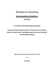
As already mentioned, SGD occurs mostly as slow and diffuse flow, but can also be a point
source like a submarine spring. The flow rate depends thereby on the permeability of the
sediments overlying the seeping aquifer (Valiela et al., 1990). SGD, as defined by (Burnett et
al., 2003), is any and all flow of water on continental margins from the seabed to the coastal
ocean, regardless of fluid composition and driving force. In addition, submarine groundwater
recharge (SGR) occurs: Tides, waves, currents, sea level fluctuations and density differences
force seawater into the sea floor. Therefore driving forces for SGD are not only the terrestrial
hydraulic gradients but also oceanic processes (Figure 1.1) which leads to the high spatial and
temporal variability. In the transition zone between fresh and saline groundwater exists a
brackish mixing zone with a salinity gradient from land to sea. (Moore, 1999) therefore
introduced the term “subterranean estuary”.
Figure 1.1: Nomenclature of fluid exchange and schematic depiction (no scale) of processes
associated with submarine groundwater discharge and recharge. Arrows indicate fluid
movement. Modified by Burnett et al. (2003) from Thibodeaux and Boyle (1987)
From 2002 to 2005 the EU project COSA was conducted on the island Sylt (North Sea,
Germany) and Hel Penisula (Baltic Sea, Poland). The aim was to investigate the role of
“COastal SAnds as biocatalytical filters”. During this project SGD was found on the beach of
the village Hel (outer Puck Bay). The present diploma thesis was conducted within the scope
of the BONUS project AMBER (Assessment and Modelling of Baltic Ecosystem Response),

Introduction 3
where one aspect deals with the biogeochemistry of the SGD in Hel and its impact on the
coastal ecosystem. In most studied cases nitrate is the dominant N species found in
groundwater (R. L. Smith et al., 2006). However, first measurements during the autumn
campaigns on Hel Peninsula in 2009 showed very high ammonium concentrations in the
groundwater seepage.
Ammonium in groundwater may naturally be generated by the anaerobic degradation of
organic matter or artificially as a result of organic waste disposal. Anthropogenic ammonium
sources may be wastewater disposal, sewage systems and agricultural practices. The transport
of ammonium in groundwater may be retarded by physical-chemical processes such as
sorption or by biological processes like microbially induced transformations, depending on
aquifer geochemistry and the nature of the groundwater flow system (Böhlke et al., 2006).
Ammonium may therefore have much longer flushing times than other more mobile aqueous
species (Ceazan et al., 1989; van Breukelen et al., 2004). Ammonium is an N source for
phytoplankton and is highly bio-available thus being assimilated by such organisms. In
addition to assimilation, transformation of ammonium may also occur by nitrification of
microorganisms. In this process ammonium is oxidized with O 2 to NO - 3 . In the transition zone
of oxic-anoxic conditions nitrate may be removed from the system by denitrification which
transforms nitrate to gaseous N 2 . Alternatively, ammonium may be oxidized anaerobically
with reduction of nitrite to form N 2 , called the anammox process (Van de Graaf et al., 1995;
Thamdrup & Dalsgaard, 2002). Inorganic N (nitrate and ammonium) is immediately available
to primary producers. Also dissolved organic nitrogen (DON) from terrestrial sources may
show substantial biological availability, but mineralization and assimilation occurs relatively
slowly (Qualls & Haines, 1992; Seitzinger et al., 2002).
To study N altering processes stable isotopes are often used. The two stable isotopes of N are
14 N and 15 N. They both have the same number of protons and electrons but the heavier 15 N
contains one more neutron. N in the atmosphere consists of 99.63 % of 14 N and 0.37 % of 15 N.
The ratio in abundance of these two natural N isotopes can give information about sources
and sinks of N (Peterson & Fry, 1987; Sulzman, 2007) because the isotope ratio 15 N/ 14 N, or R,
varies among different N pools. Since those differences are very small the isotopic
composition is reported as the deviation of R from a sample from R of a standard in parts per
thousand:

Introduction 4
δ
15
N(‰)
=
⎛
⎜
⎝
R
R
sample
s tan dard
⎞
−1
⎟ ∗ 1000
⎠
[1.1]
It is possible to discriminate the N source of a sample if the pools to be considered are distinct
in their δ 15 N values.
Stable isotopes may also be used to identify N altering processes because of the occurring
fractionation during a reaction. This is because more energy is needed to break bonds in
molecules with the heavier 15 N isotope. Since 15 N therefore has a lower reaction rate than 14 N,
it is discriminated over 14 N in biochemical reaction leaving the remaining substrate enriched
in 15 N compared to the product. This can be expressed in the following way, where ε p/s is the
isotope enrichment factor:
δ +
15
15
N
product
≅ δ N substrate
ε
p / s
[1.2]
Processes altering NH + 4 concentration, like nitrification, show different fractionations. Simple
mixing of NH + 4 into a NH + 4 free solution would not change the isotope ratio and ε is therefore
0 ‰, while ε for the assimilation of NH + 4 by marine diatoms was found to be -20 ± 1 ‰
(Waser et al., 1998). The isotope enrichment factor for nitrification may range from -17 to -38
‰ (Mariotti et al., 1981). Sorption of NH + 4 in sediments to clay for instance leads to an
opposite fractionation. NH + 4 remaining in solution gets enriched in 14 N with ε being +1 to +11
‰ (Delwiche & Steyn, 1970; Karamanos & Rennie, 1978).
Isotope ratios can also be helpful for analyses of food webs. In this case the carbon (C)
isotopes can give information about the food source of organisms. The two stable C isotopes
are 12 C and 13 C and the δ 13 C values of animals reflect there diets within about 1 ‰ (DeNiro &
Epstein, 1978; Rau et al., 1983; Peterson & Fry, 1987). N on the other hand shows a more
significant enrichment of 15 N between a consumer and its diet (DeNiro & Epstein, 1981).
Isotope ratios of N can therefore be used to identify the trophic level of animals in a food web.
Minagawa & Wada (1984) found a mean 15 N enrichment of +3.4 ± 1.1 ‰ per trophic level
independent of the habitat and according to Peterson & Fry (1987) animals are 3 to 5 ‰
heavier in the isotopic composition of N than their diets. On average field studies have shown
an enrichment of 3.2 ‰ per trophic level (Post, 2002). Stable isotopes of organisms may also
reflect differences in the N source of primary producers. McClelland et al. (1997) found that

Introduction 5
producer and consumer 15 N/ 14 N ratios were both shifted due to isotopically heavy wastewater
N inputs.
In the present diploma thesis DIN concentrations as well as δ 15 N values of DIN and organic
forms of N have been used to understand the ecological importance of SGD to the Puck Bay.
Therefore the following hypotheses are worked out:
1. δ 15 N-NH 4 + values are different to all other N sources..
2. The entry of nitrogen via SGD is temporally, seasonally and spatially very variable and
enters the coastal waters unmodified. SGD at Hel Peninsula contributes significantly to the N
input into the Puck Bay.
3. The δ 15 N signal can be detected in the trophic network.

Material and Methods 6
2 Material and Methods
2.1 Sampling Site
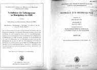
Figure 2.1: Map of the western part of the Bay of Gdańsk with Puck Bay. The broken line
indicates the underwater sandy bank separating Puck Lagoon from the outer Puck Bay.
Arrows indicate the river mouths of Vistula and Reda. Sampling sites were the beach of the
village Hel (") and a reference station at the Baltic Sea side of Hel Peninsula (").

Material and Methods 7
Sampling took place on Hel Peninsula in Poland. It is a 36 km long sandy spit which forms
Puck Bay, the south western part of the Bay of Gdańsk (Baltic Sea) (Figure 2.1).
Puck Bay is a semi-enclosed gulf characterized by low average salinities of 7.6 (Nowacki,
1993). Depths range from 2 m in the western part of the Bay to 50 m in the eastern part
(Nowacki, 1984). Puck Bay is divided by an underwater sandy bank into the inner shallower
Puck Lagoon (average depth 3.1 m) and the outer Puck Bay (average depth 20.5 m). This
bank is divided by two straits where intensive water exchange between outer Puck Bay and
Puck Lagoon occurs.
The bay is influenced by marine waters from the Gulf of Gdańsk as well as by terrestrial
waters. 76.3% of the whole Puck Bay catchment area drains into Puck Lagoon. Puck Bay is
classified as eutrophic. It is polluted with wastewaters from three sewage treatment facilities
and seven rivers (Kruk-Dowgiałło & Szaniawska, 2008) the largest being the Reda River. The
annual N input into Puck Bay is 2,275 t a -1 (Pempkowiak, 1994). The average inflow of wet
nitrogen from the atmosphere was estimated to be 306,040 t (Bolałek et al., 1993).
Furthermore high flux rates up to 1434 µmol NH 4 -N m -2 day -1 from sediment to bottom water
were found within the Puck Bay (Bolałek & Graca, 1996) leading to an amount of about 825 t
NH 4 per year passing from the sediment to near-bottom water. Approximately 205,400 t
inorganic N (IN) flow from the Gulf of Gdańsk into Puck Bay annually. Outflow of
substances occurs mainly in winter being 197,600 t IN a -1 (Kruk-Dowgiałło & Szaniawska,
2008).
Hel Peninsula has evolved during the Holocene. Its coast consists basically of recent alluvial
and littoral zone Holocene sediments (Furmanczyk, 2007). Pleistocene deposits are present in
the substratum of the whole spit (Tomczak, 1995). In the eastern part of the spit where
sampling took place, the Holocene series is fully developed with a thickness up to 100 m
(Figure 2.2). The surficial bottom sediments of the coast around the head of the spit (study
area) consist mainly of medium-grained sands (Kramarska, 1995).
The bottom sediments of Puck Bay consist mainly of sand and mud (Krzymiński et al., 2004).
There are at least three main ground water horizons underlying Puck Bay: One upper
Cretaceous, one Tertiary and one Quaternary horizon. Puck Bay is the main drainage area for
those aquifers (Dowgiałło & Kozerski, 1975; Sadurski, 1986).
Seismoacoustic profiling showed a series of permeable deposits under the sea floor
(Jankowska et al., 1992). Since the groundwaters of the three aquifers are fresh, the existence
of drainage zones is indicated by changes in the salinity of the sediment-water interface. SGD
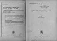
into the Puck Bay occurs mainly by ascensic seepage through the seabed (Figure 2.2). On Hel

Material and Methods 8
Peninsula the Cretaceous aquifer, which is generally isolated from the overlying horizons, is
in direct contact with the Pleistocene sandy series and constitutes a joint groundwater horizon
(Jankowska et al., 1994). The cross-section in Figure 2.2 presents a relatively simple
illustration of the existing conditions. The actual hydrogeology might be far more
complicated.
Winds from north northwest are the most important physical process that causes erosion along
Hel Peninsula and create a transport of sediments along the shore towards the end of spit.
North-easterly winds, perpendicular to the spit, create currents that transport sandy material
eroded from the coast into deep water (Furmanczyk & Musielak, 1999). The eastern part of
Hel Peninsula with the sampling area is predominantly accumulating (Furmanczyk, 1994).
There are on. Besides built-up areas and railway there are forests, meadows and wastelands
on Hel Penisula but no arable fields. The three important sectors of economy on Hel
Peninsula are fishery and fishing industry, tourist industry and defence and military services
(Furmanczyk, 2007).
Figure 2.2: Hydrogeological section through Puck Bay from Gdynia to Hel. Sediment depth
is given as meter below sea level (m b.s.l.). The three aquifers with the direction of the
groundwater flow are indicated by the green arrows. From bottom up: Cretaceous, Tertiary
and Quaternary horizon. Vertical green arrows indicate potential submarine groundwater
discharge. The sampling site in Hel and the 180 m deep sampled well are shown. (modified
from Piekarek-Jankowska (1996))

Material and Methods 9
The main sampling site was on the beach of the village Hel on Hel Peninsula. Altogether 5
sampling campaigns were conducted: Two in September and November 2009, one in the end
of February till the beginning of March 2010 and two in May and October 2010. During
October 2010 samples were taken from the Baltic Sea side of Hel Peninsula as a reference
station (Figure 2.1), too.
2.2 Sampling
Pore water salinity was tested at first in the research area to find spots with SGD. This was
done with the help a push pull lance (Figure 2.3). Such a lance is very thin (about 1 cm in
diameter), has only one port at the lower end and can be pushed into the sediment and
sampled immediately.
At spots with low pore water salinities larger groundwater lances were buried in the sediment
(Figure 2.3) to sample submarine groundwater. These groundwater lances had each 8 ports all
located in different heights. The difference in height between the ports constitutes 4 cm,
respectively, except for the two lowest ports (7 and 8) where the difference was 8 cm (Figure
2.3). Since the burial disturbed the sediment this lances could not be sampled immediately.
Only after at least 24 hours the sediment was thought to be readjusted and samples could be
taken from different depths with syringes via the Teflon tubes. It was not possible to plunge
the lances completely into the sediment. Thus only the lower five to six ports were connected
to the pore water and could be sampled (Figure 2.3). Groundwater lances were sampled on
two to three different days. From every port 100 to 200 ml could be sampled (Table 2.1).
In September and November 2009 samples for N measurements were taken by S. Vogler
(Institute for Baltic Sea Research, Working Group: Geochemistry and Stable Isotope
Geochemistry) from one groundwater lance, respectively. For the February/March campaign
no samples were available. The May and October campaigns were planned and conducted by
myself as well as all N measurements.

Material and Methods 10
Figure 2.3: Sampling lances used in Hel. Each port is connected to one Teflon tube. Pore
water was taken from the Teflon tubes with the help of syringes. The groundwater lances had
8 sampling ports in different heights. The thinner push pull lance had only one port at the
lower end.
During May and October 2010 transects were sampled in addition to the groundwater lances
within the SGD impacted area perpendicular to the beach line (Figure 2.4). Since only two
groundwater lances were available, this was done using the thinner push pull lances (Figure
2.3). During the last two campaigns in May and October bottom and surface water was taken
at each pore water sampling site.
In October 2010 the Baltic Sea side of Hel peninsula was sampled in addition. Pore water
samples were taken with a push pull lance together with water column samples. Only one
sediment depth (30 cm) was sampled at two adjacent spots.

Material and Methods 11
Figure 2.4: Sampling sites on the beach of the village Hel. Beach with shoreline as existent
during October 2010. During May the shore line was farther east as indicated as the broken
green line. Ground water lances (L) and push pull lances (T). Rope from which organisms
were collected (R). Benthic chambers (BC) Locations during September 2009 ("), May 2010
(/) and October 2010 (,). No location coordinates were available for November 2009 and
February/March 2010, here two ground water lances were placed each time similar to the sites
during September 2009.
Two wells were sampled in addition: One 3 m deep well at the Fokarium Stacji Morskiej in
Hel as well as a 180 m deep well at the drinking water treatment plant in Hel.
In October 2010 six benthic chambers were positioned in a circle (ca. 1 m in diameter)
between the two groundwater lances (Figure 2.4). They were used to measure the
groundwater and ammonium fluxes between the sediment and the water column. Chambers
were 330 mm in height and 190 mm in diameter (Figure 2.5). They were placed on the
sediment-water interface by pushing them about 15 to 20 cm deep into the sediment. Height
of the enclosed water column above the sediment was about 15 cm. A stirrer was installed to
create an advective flow within the chamber. Water samples were taken with syringes from
the sampling valves. Incubation was conducted from October 6 th at 15.45 till the next day at
16.30. Sampling took place at the start and stop of the incubation. In addition samples were

Material and Methods 12
taken on October 7 th at 08.05 marking the end of the dark incubation (from 15.45 till 08.05)
and the start of the light incubation (from 08.05 till 16.30). At every sampling point 50 ml
were taken from each chamber.
Table 2.1: Samples taken during the different campaigns from groundwater lances (L), push
pull lances along transects (T) benthic chambers (BC) and wells. The range of sampled
sediment depths is given for all lances as well as the number of sampling days for the
groundwater lances. *There were no samples available for February/March, but ammonium
concentrations were provided by S. Vogler.
Sampling
Campaign
L1
depths
(cm)
Groundwater lances
sampl.
days
L2
depths
(cm)
sampl.
days
Nb.
Transects
T
depths
(cm)
Sample
V per
port (ml)
Sepember 2009 - - - x 4 to 24 2 - - - 100
November 2009 x 4 to 28 1 - - - - - - 100
Feb/March 2010* - - - x 4 to 28 2 - - - -
May 2010 x 4 to 40 2 x 4 to 40 2 1 T1 to T4 5 to 30 100
October 2010 x 4 to 28 2 x 4 to 28 3 2 T1 to T3 5 to 20 200
T4 to T6 5 to 20 200
Sampling
Campaign
Nb. of
lances
Baltic Sea side BC Wells
depths
(cm)
Sample V
per port
(ml)
Nb. of
BC
Sample
V per BC
(ml)
3 m
deep
Sepember 2009 - - - - - - -
November 2009 - - - - - - -
Feb/March 2010* - - - - - - -
May 2010 - - - - - x -
October 2010 2 30 200 6 50 x x
180 m
deep
All water samples were filtered and salinity and NH +
4 concentration were measured
immediately. Subsamples for NO x and DON concentration measurements as well as for the
determination of δ 15 N in NH + 4 were stored frozen in PE bottles at -20°C. Water column
samples were filtered on GF/F filters and stored frozen until analyses.

Material and Methods 13
Figure 2.5: Schematic diagram of the benthic chambers used to measure the groundwater and
ammonium fluxes between the sediment and the water column during the October campaign.
The chamber depicted shows the experimental set-up during pre-incubations. Plastic spacers
were removed before incubation start and chambers closed with Lids. (from Cook et al.
(2005))
Organisms were sampled during October 2010. Plankton was sampled from the SGD
impacted site of the beach in Hel as well as from the Baltic Sea side of Hel peninsula.
Phytoplankton was collected with a 10 µm mesh size net and filtered on GF/F. Zooplankton
samples were collected with a 55 µm net and living zooplankton was separated from seston
and phytoplankton. Therefore the whole net sample was filled in an opaque dark chamber
which was connected via a pipe with a transparent light chamber filled with filtered seawater.
The living zooplankton was moving into the light chamber and thus separated from the rest of
the sample. All plankton samples were stored frozen at -20°C until analyzing. Benthos was
collected from the same sites as plankton using a brailer. In addition ropes anchored in the
sediment were found on the beach of Hel near the groundwater lances (Figure 4) and on the
Baltic Sea side. Parts of them were cut off and epiflora and epifauna were hand picked.
Benthic animals were held in filtered seawater for 24 hours to allow their guts to clear. All
benthos samples were classified and stored frozen separately at -20°C till analyzing.
Sediment from the first 20 cm was taken at the SGD impacted site for a lab experiment. It was
transported in a bucket with some supernatant seawater from the Puck Bay. At IOW it was

Material and Methods 14
kept at a 4°C cooling chamber spread in a basin with supernatant seawater until conduction of
the experiment.
2.3 Laboratory experiment with artificial sediment cores
To investigate the potential for nitrification at the sampling site a core experiment was
conducted. Sediment cores were streamed with nutrient-poor seawater with added ammonium.
The experiment was set up in the following way. Eight PE tubes (length 25 cm, diameter 2.4
cm) were closed on both ends with plugs, which were perforated with Tygon hoses (Figure 6).
A perforated washer was placed over the lower plug with a GF/F filter on top to avoid
sediment to fall through. The PE tubes were half filled with nutrient-poor seawater through
the Tygon hose at the lower end with the help of a peristaltic pump (MCP Standard).
Afterwards the PE tubes were filled with the homogenized sediment taken from Hel. The
Sediment cores were 18 cm high. Before the start of the experiment the water in all cores was
exchanged with nutrient-poor seawater (pump velocity 2ml min -1 for 1 hour). After this the
experiment was started. Two control experiments were performed with nutrient-poor seawater
only. The other six cores were performed with nutrient-poor seawater with added ammonium
chloride. In three cores NH + 4 concentration of the solution was 200 µmol L -1 in the other three
500 µmol L -1 . The experiment was carried out until the pore water in the sediment was
exchanged once. The time needed for that was calculated prior to the start of the experiment
by determination of the pore volume:
t
=
V
v
P
[2.1.a]
V
P
= V K
∗φ
[2.1.b]
Vol%
φ =
100
[2.1.c]
Vol%
=
WW − DW
∗100
1.011
WW − DW DW
+
1.011 2.65
[2.1.d]

Material and Methods 15
t indicates the time needed for one pore water exchange at a certain pump velocity v for the
pore volume V P in the sediment core. V K depicts the volume of the sediment core and ø the
porosity of the sediment which is calculated from the water content in volume % (Vol%).
Equation 2.1.4 gives the calculation of Vol% for sandy quartz sediments and seawater. WW
indicates the wet weight and DW the dry weight.
For the experiment this results in the following:
ø = 0.38
V K = 163,4 cm 3 (area A = 9.1 cm 2 , height l = 18 cm)
V P = 62.6 cm 3 (= 62.6 ml)
v = 0.108 ml min -1 t = 580 min = 9.7 h 40 min
v = 0.05 ml min -1 t = 1252 min = 20 h 52 min
The experiment was conducted twice at the two different pumping velocities 108 µl min -1 and
50 µl min -1 . These velocities were chosen because they were similar to the seepage rates
measured in Hel. The exact pumping velocities were determined by the pump and the
diameter of the pumping hoses.
The experiments were stopped after the water exchange. The water above the sediment cores
was completely collected. In the end of the experiment the pore water of the sediment was
pumped downwards and collected as well. During each experiment oxygen saturation was
measured continuously with an oxygen microelectrode (Figure 2.6) in the water above the
upper end one of the eight cores. NH + 4 and NO x concentrations as well as δ 15 N-NH + 4 values
were measured in all samples from the core experiments. δ 15 N-NH +
4 of the ammonium
chloride solution used was measured, too.

Material and Methods 16
Figure 2.6: Experiment set up. Shown is one core. 18 cm of Sediment was filled into the PE
tube. Solution was pumped with a tubing pump through the sediment. Flow direction is
indicated. Oxygen saturation was measured at the end of one of the eight cores.
The isotopic enrichment factor for nitrification can be calculated after (Mariotti et al., 1981).
The following calculations were applied:
δ
s
= ε
p / s
∗
ln
f
[2.2.a]
δ s denotes for the δ 15 N-NH 4 + value of the sample. ε p/s is the isotopic enrichment factor.

Material and Methods 17
f =
N
N
s
s,0
[2.2.b]
N s,0 is the NH + 4 concentration at the start in the solution. N s is the NH + 4 concentration of the
sample.
For every δ s three data points were available with each three parallels: One from the starting
solution, one from the cores and one from the supernatant solution on top of the cores.
2.4 Analytical methods
2.4.1 Determination of DIN
All DIN measurements of the samples from September and November 2009 were conducted
+
by F. Korth (Institute for Baltic Sea Research, Working Group: Stable Isotopes). NH 4
concentrations from additional samples during these campaigns were measured by S. Vogler
and were also available. For the February/March campaign no samples were available but
NH + 4 concentrations measured by S. Vogler are presented in the results part.
For measurements of DIN concentrations the colorimetric determination of NO - 2 , NO - 3 and
NH + 4 after (Grasshoff et al., 1983) was applied.
The determination of NH + 4 was carried out photometrically as indophenol blue. NH + 4 reacts
in moderately alkaline solution with Trione (dichloroisocyanuric acid) to monochloramine
leading to indophenol blue in presence of phenol. After six to 18 hours the extinction was
measured at 630 nm. As sulphide concentrations higher than 2 mg/l interfere with this method,
pore water samples were diluted accordingly.
NO 2
-
was determined with 5 ml for each water column sample. NO 2
-
reacts with
Sulphanilamide hydrochloride forming a diazonium compound. This couples with N-(1-
naphtyl)-ethylenediamine dihydrochloride leading to the formation of a red azo dye. The
colour intensity is thereby proportionally to the NO - 2 concentration. After 15 minutes in the
dark the extinction was measured photometrically within a 5 cm semi micro cell at 543 nm.
NO - 3 within water column samples was reduced to NO - 2 in copper-plated cadmium columns
at a pH between 7.5 and 8.4. The samples were then further treated as explained for NO - 2 .
NO 3
-
and NO 2
-
concentration in pore water samples were determined with the “Spongy
Cadmium method” (Jones, 1984). Samples are buffered at pH 8.5 and shaken for 90 minutes

Material and Methods 18
with spongy cadmium. NO 3
-
is reduced to NO 2 - . Color reagent B is added and after 15
minutes in the dark extinction for combined NO 3 - and NO 2 - is measured at 543 nm.
2.4.2 Determination of DON
Dissolved organic nitrogen (DON) was measured indirectly by determination of total
dissolved nitrogen (TDN) in filtered samples applying the persulfate oxidation method after
(Grasshoff et al., 1983). 40 ml of the water sample was transferred into PTFE-tubes,
respectively and 10 ml of potassium peroxide solution was added. All nitrogen within the
sample was then digested to nitrate in a microwave (CEM, MarsXpress) for 30 minutes at 180
to 200°C. Nitrate representing TDN was determined after oxidation with the Spongy
Cadmium method as described in the section above. DON was then calculated by the
difference of TDN minus DIN of the sample measured before. For DIN/TDN ratios >0.85 the
standard deviation on DON measurements increases greatly (Vandenbruwane et al., 2007).
Hence, NH + 4 had to be removed from pore water samples with high NH + 4 concentrations
before digestion. This was done by applying NH + 4 diffusion method (see below). Afterwards
the filter was removed and the solution was filtered prior to DON measurements. To eliminate
the filtering step after the diffusion it was tried to raise pH with NaOH instead of MgO. But
since the pH was sinking below 9.7 in the presence of NaOH and without MgO during
incubation, this method was abandoned again. Due to time issues it was not possible to
measure DON concentrations in all samples and the error of the DON measurement due to the
removal of ammonium could not be determined exactly.
2.4.3 Stable Isotopes
Ammonium
Isolation of NH + 4 from the samples to determine δ 15 N values was conducted in two different
ways. For pore water samples the NH + 4 diffusion method (Sigman et al., 1996) was applied.
Samples were transferred into Schott flasks and MgO was added to increase pH as well as a
pack of Teflon membranes containing an acidified GF filter. The Schott flask is closed
immediately and held in a shaking water bath for 5 days. At pH higher than 9.7 the acid-base
pair, NH + 4 -NH 3 is present as the gas NH 3 which then diffuses through the Teflon membranes
onto the acidified filter. NH 3 is converted to NH + 4 at low pH and remains on the filter which
is stored in a desiccator for at least two days. Prior to analysis the filters were removed from
the Teflon membranes, dried at 60 °C over night and then folded into tin cups.

Material and Methods 19
Due to low NH + 4 concentrations in water column samples the diffusion method was not
suitable and therefore the NH + 4 distillation method after (Velinsky et al., 1989) was applied.
As explained for the diffusion method MgO is added to the sample to shift the equilibrium of
NH + 4 -NH 3 towards NH 3 . During distillation the NH 3 evaporates from the sample and is
collected in a measuring cylinder containing a weak acid which traps NH 3 as NH + 4 again.
This distillate is then mixed with a molecular sieve which collects all NH + 4 within the solution.
The molecular sieve was filtered onto a precombusted GF/F filter (450 °C for 3 h) and dried at
60 °C over night. The molecular sieve was removed from the filter and transferred into a tin cup.
For the benthic chambers 4 to 6 δ 15 N values are missing due to low NH + 4 concentrations and
sample volumes for the samples from the start of incubation.
POM and Organisms
Benthos samples were dried and homogenized with mortar and pestle before measurements
on the mass spectrometer. Small animals were measured as a whole directly after drying.
From calcareous organisms like mussels and barnacles the shells were removed and the
remains acidified prior to measurements. Filters for particulate organic matter (POM) and
plankton samples were dried and measured directly. All samples were transferred into tin cups
for analyses of δ 15 N, δ 13 C and C/N values.
2.5 Mass spectrometric analyses
Tin cups were pressed into pellets and measured in an elemental analyser (flash EA) coupled
to an isotope ratio mass spectrometer (IRMS, Finnigan Delta S). The samples are combusted
with additional oxygen at 1020°C (flash combustion) converting all inorganic and organic
nitrogen and carbon into gases. The carrier gas helium transports these combustion gases
through a reduction furnace (650°C) where NO x is reduced to N 2 . To remove water before
transporting the gases to a gas-chromatographic column which separates N 2 from CO 2 , the
helium flow passes a water trap. A subsample (~ 1%) is transferred into the IRMS were the
gases are ionized and accelerated before entering the magnetic sector. The ions are separated
depending on their charge ratio and hit a collector. A detector transforms the electric signal.
All isotope values are noted relative to reference gases (N 2 , CO 2 ,):

Material and Methods 20
δ
15
N
⎡ ⎛
⎢
⎜
⎢ ⎝
⎢⎛
⎢
⎢
⎜
⎣⎝
15
14
sample
[‰] =
∗1000
15
14
N ⎞
⎟
N ⎠
N ⎞
⎟
N ⎠
reference
⎤
⎥
⎥
⎥
⎥
⎥
⎦
[2.3]
This way the mass spectrometer measures the difference in 15 N abundance between sample
and reference. The reference gasses are calibrated against international standards of the
International Atomic Energy Agency (Table 1).
Table 1: Overview over IAEA standards and internal lab standards.
Standard δ 15 N (‰) δ 13 C (‰)
international standards
IAEA N1 (Ammonium sulphate) 0,43 ± 0,07
IAEA N2 (Ammonium sulphate) 20,32 ± 0,09
IAEA N3 (Potassium nitrate) 4,69 ± 0,09
IAEA C6 (Saccharose) -10,43 ± 0,13
NBS22 (Oil) -29,74 ± 0,12
internal laboratory standards
Peptone 5,8 ± 0,2 -22,11 ± 0,17
Acetanilid -1,7 ± 0,2 -29,81 ± 0,19
2.6 End-member mixing calculations
To investigate mixing patterns of groundwater and marine NH + 4 the conservative mixing
equations by (Fry, 2002) were applied. The concentrations of NH + 4 -N were modelled as
mixture (C MIX ) of groundwater and Puck Bay water column end-members:
C
MIX
= f ∗C
+ 1
GW
( − f ) ∗CP
[2.4a]
C denotes the NH + 4 concentration. The subscript GW indicates the groundwater end-member
and the subscript P the Puck Bay water column end-member. f is the fraction of freshwater
calculated from salinity (S):

Material and Methods 21
f
=
S
P
− S
S
P
MIX
[2.4b]
Water column end-members were calculated from the means of all water column samples
during each campaign. As groundwater end-member the well samples were used. In addition
mixing was calculated with pore water samples with the lowest salinity during each sampling
campaign as groundwater end-member. However, pore water samples present no true
groundwater end-members. As they all had salinities >0, f had to be adapted as followed:
f
=
S
S
P
P
− S
− S
MIX
GW
[2.4c]
The conservative mixing of 15 N-NH 4 + values (δ MIX ) was calculated as well:
δ
MIX
=
f
∗C
GW
∗δ
GW
+
C
( 1−
f )
MIX
∗C
P
∗δ
P
[2.4d]
δ denotes the NH + 4 isotopic values. End-members were achieved in the same way as for
concentration mixing.
Deviations of actual samples from the theoretical conservative mixing lines indicate
additional sources or sinks in the mixing gradient. For the concentration mixing that means
higher values than predicted point towards additional sources and lower values towards
additional sinks.

Results 22
3 Results
3.1 Seasonal and temporal variability
For the characterization of the submarine groundwater discharge salinities and nitrogen
compounds are presented. In addition sulphide was measured during the May and October
campaigns and provided by Susann Vogler.
Seasonal variations are shown in depth profiles of the groundwater lances sampled during all
campaigns (Figure 3.1). The number of parallels for each sampling campaign varied between
one and five (Table 3.1).
Figure 3.1: Depth profiles from pore water and water column samples of groundwater lances
during the different sampling campaigns. Horizontal lines at 0 cm depth indicate the sediment
surface. Salinity (A), ammonium (NH 4 + ) (B), sum of nitrite and nitrate (NO 2/3 - ) (C), dissolved
organic nitrogen (DON) (D) and sulphide (S -2 ) (E) from the different seasons. Means and
standard deviations are given. September 2009 (,), November 2009 (/), March 2010 (&)
May 2010 (/), October 2010 (,). Note break in x-axis of 3.1B.

Results 23
Table 3.1: Number of sampling parallels from groundwater lances during each sampling
campaign.
Sampling Campaign
Nb. of
groundwater
lances
Nb. of
sampling days
Overall sampling
parallels
September 2009 1 2 2
November 2009 1 1 1
February/March 2010 1 2 2
May 2010 1 2 2
October 2010 2 2, 3 5
Highest salinities of 6 to 7 were measured in the water column and decreased below 2 with
increasing depth. Only in November 2009 the lowest measured salinity was 2.4. The strongest
decrease down core occured within the first 10 to 15 cm. In this zone the highest variability
between sampling days was encountered. Ammonium concentrations were lowest in the upper
water column ranging from 1 to 4 µmol L -1 . They were increasing with depth and decreasing
salinity. Highest values were measured during November 2009 reaching 5.8 mmol L -1 in 20
cm depth. Ammonium depth profiles from March and October 2010 showed much lower
concentrations of 600 to 800 µmol L -1 at 28 cm depth but were quite similar to each other.
Lowest concentrations were measured during September 2009 (on average 310 µmol L -1 at 24
cm depth) and May 2010 (235 µmol L -1 at 40 cm depth). The sum of nitrite and nitrate (NO - 2/3 )
concentrations were low at the sediment surface (3 to 5 µmol L -1 ) and decreased mostly below
1 µmol L -1 within the first 10 cm in the sediment. Values around 8 µmol L -1 were only found
in the water column during October 2010. A peak of 2.5 µM NO - 2/3 was found in May at 8 cm
sediment depth. DON concentrations ranged between 10 and 40 µmol L -1 but showed no
trends with depth. Sulphide values measured during May and October 2010 increased with
depth. In May they reached a maximum of 23 µmol L -1 at 24 cm depth. In October sulphide
values were lower reaching only 9 µmol L -1 at 20 cm depth.
Ammonium concentrations plotted over the salinity showed the mixing behaviour of
ammonium from SGD (Figure 3.2). The theoretical conservative mixing lines (after Fry 2002)
for the two sampled wells and the pore water samples are given (for calculations see
equations 2.4 to 2.7). The mean values from all water column samples taken during each
campaign were used as saline end-members, respectively. Values from the well samples as
well as from pore water samples with the lowest salinity during each campaign were used as
groundwater end-members (Table 3.2). Both wells contained relatively low ammonium
concentrations, 26.8 µmol L -1 in the 3 m deep well and 32.6 µmol L -1 in the 180 m deep well.
The data from the pore water samples did not fit those two mixing lines. Despite some scatter

Results 24
the mixing of ammonium concentrations was mostly conservative as predicted by each pore
water mixing line. For the data points from pore water samples the linear regression lines (y =
a*x + b) were calculated and compared to the respective conservative mixing lines, which
were also linear with the simple equation y = a*x + b (Table 3.3). Samples from November
2009 and February/March 2010 showed fewest scatter and the linear regression had the
highest r 2 r of 0.99 and 0.95, respectively. The conservative mixing lines and the sample
regression lines were quite similar for those two campaigns. In November 2009 the slope (a)
of the sample regression line was slightly steeper than that of the conservative mixing line
(a r /a m = 1.05). In February/March 2010 it was the other way around (a r /a m = 0.92). Most data
were available from the October 2010 campaign. They varied mostly between salinities of 0
to 2 with differences in ammonium concentrations of about 400 µmol L -1 at salinity 1.
However r 2
r of the sample regression line were still relatively high with 0.93. The
conservative mixing line and the sample regression line of October 2010 showed the highest
similarity (a r /a m = 1.01) between all sampling campaigns. There was also scatter in the May
2010 data. r 2 r was only 0.71 for the sample regression line. a r /a m for this month was only 0.87
showing a steeper slope of the conservative mixing line than of the sample regression line.
The highest variations between data were found in September 2009. The sample regression
line had the lowest of all r 2 r (0.57). For this month also the maximum difference between
conservative mixing line and sample regression line (a r /a m = 0.70, b r /b m = 0.71) was found.
Table 3.2: End-members for the calculations of conservative mixing of ammonium (NH + 4 )
concentrations. Seasonal samples. Sediment depths of all groundwater end-members are given
as well as the distances from the sediment surface of the respective water column samples for
the Puck Bay end-members.
Groundwater end-member Puck Bay end-member
Groundwater lances
Samples
Sediment
depth (cm)
Salinity
NH 4
+
(µmol L -1 )
cm above
the
Sediment
Salinity
NH 4
+
(µmol L -1 )
September 2009 24 1.1 479 1 7.2 3
November 2009 28 2.4 5478 1 7.3 242
February/March 2010 28 0.4 816 1 6.9 1
May 2010 24 0.5 226 10 to 60 6.9 2
October 2010 28 0.3 678 10 to 80 6.3 4
Well 3m (Oct. 2010) 300 0.0 27 10 to 80 6.3 4
Well 180m (Oct. 2010) 18,000 0.0 33 10 to 80 6.3 4

Results 25
Figure 3.2: Ammonium (NH 4 + ) concentrations over salinity. Two wells sampled in October
2010 (3 m deep ", 180 m deep ") and groundwater lances sampled in September 2009 (,),
November 2009 (/), March 2010 (&) May 2010 (/) and October 2010 (,). Conservative
mixing lines for pore water of every month and the two wells. For end-members see Table 3.2.
Note break in y-axis.
Table 3.3: Comparison of regression lines calculated from conservative end-member mixing
and sample data for groundwater lances. Equation for regressions: y = ax + b. a (slope) and b
are given for all equations. Subscript m indicates the mixing calculation and r the sample
regression line. For sample regression lines r 2 and number (nb.) of samples are given in
addition. r 2 for all end-member mixing regressions is 1. a r /a m shows the relation of the slope
of the sample regression to that of the mixing calculation.
Mixing calculation Sample regression line
Samples
a m b m a r b r r r
2 nb. of
samples
a r /a m
b r /b m
Groundwater lances
September 2009 -77.4 562.5 -54.5 398.7 0.57 12 0.70 0.71
November 2009 -1067.5 8041.2 -1116.5 8275.0 0.99 5 1.05 1.03
February/March 2010 -124.9 869.1 -114.9 835.8 0.95 13 0.92 0.96
May 2010 -34.7 241.6 -30.3 219.1 0.71 16 0.87 0.91
October 2010 -111.7 711.5 -112.9 718.4 0.93 38 1.01 1.01
Well 3m (Oct. 2010) -3.7 26.8
Well 180m (Oct. 2010) -4.6 32.6

Results 26
3.2 Spatial variability
The depth profiles of lances sampled in transects perpendicular to the shore line during May
and October 2010 showed the spatial variability (Figures 3.3 and 3.4). The May transect was
about 30 m long whereas the two October transects were each about 15 m long. For positions
of lances see Figure 2.4.
Figure 3.3: Depth profiles of lances sampled in a transect perpendicular to the shore line in
May 2010. Salinity (A), ammonium (NH 4 + ) (B), sum of nitrite and nitrate (NO 2/3 - ) (C),
dissolved organic nitrogen (DON) (D) and sulphide (S 2- ) (E). Horizontal lines at 0 cm depth
indicate the sediment surface. Adjacent lances with similar values were pooled. Means and
standard deviations are given. For positions of lances see Figure 2.4. M1=T1+L1 (,), M2=T2
(/), M3=T3+L2 (,), M4=T4 (/). Note break in x-axis of 3.3B.
Adjacent lances with similar depth profiles were pooled for illustrations. M depicts for areas
of pooled lances during May 2010, O for those areas during October 2010. M1 contains
lances L1 and T1 and M3 is the mean of lances L2 and T3 sampled in May 2010. M2 includes
only the push pull lance T2 and M4 only T4. The two groundwater lances L1 and L2 sampled
in October 2010 are combined to O2. O1 includes the two push pull lances T2 and T4

Results 27
positioned closest to the shore line. O3 is the mean of the push pull lances T1, T3, T5 and T6
which were positioned farthest away from the shore line.
Figure 3.4: Depth profiles of lances sampled in two transects perpendicular to the shore line
in October 2010. Water column samples were taken on every position from 10 cm above the
sediment. Salinity (A), ammonium (NH 4 + ) (B), sum of nitrite and nitrate (NO 2/3 - ) (C),
dissolved organic nitrogen (DON) (D) and sulphide (S 2- ) (E). Horizontal lines at 0 cm depth
indicate the sediment surface. Adjacent lances with similar values were pooled. Means and
standard deviations are given. For positions of lances see Figure 2.4. O1=T2+T4 (/),
O2=L1+L2 (,), O3=T3+T1+T5+T6 (/)
During May 2010 (Figure 3.3) salinities decreased at station M1 and M3 down to 0.2,
whereas at station M2 and M4 lowest salinities were 3.4. M4 showed highest ammonium
concentrations to 1400 µmol L -1 within the first 5 cm of the sediment. Highest concentrations
in samples from M3 reach 220 µmol L -1 . Concentrations in M1 and M2 were lower, reaching
only 11 and 38 µmol L -1 , respectively. NO - 2/3 concentrations remained under 5 µmol L -1 . The
highest concentrations were found in the first centimetres of the sediment. DON
concentrations showed a high variability over depth and no linear trend with increasing depth.
Values range from 10 to 50 µmol L -1 . Sulphide concentrations exceeded 1000 µmol L -1 at M2

Results 28
and M4 at sites with salinities >3.4. Samples of M1 also contained high sulphide
concentrations of up to 500 µmol L -1 while concentrations at M3 did not exceed 10 µmol L -1 .
In general, transects sampled during October 2010 (Figure 3.4) showed a similar pattern as
the one in May. Over all there was a decrease of salinity with increasing depth. The lowest
salinity of 0.4 was found at site O2. At site O1 the salinity decreased down to 3 and at site O3
to 5. The ammonium concentrations were increasing with depth and from O1 (50 µmol L -1 ) to
O3 (on average 1500 µmol L -1 -
). They are altogether higher than during May 2010. NO 2/3
concentrations were very similar at all sampling sites. They were about 8 in the water column
and decreased with depth being smaller than 1 µmol L -1 10 cm deep in the sediment. DON has
only been analyzed of a few samples. At O1 and O2 samples varied between 17 and 27 µmol
L -1 . The only available pore water DON concentration for site O3 at 20 cm depth was 39
µmol L -1 and two fold higher than the water column concentration of 19 µmol L -1 . Sulphide
concentrations were below 10 µmol L -1 in samples from O2, but reach 2 to 4 mmol L -1 at sites
O1 and O3.
Table 3.4: End-members for the calculations of conservative mixing of ammonium (NH + 4 )
concentrations. Transects in May and October 2010. Sediment depths of all groundwater endmembers
are given as well as the distances from the sediment surface of the respective water
column samples for the Puck Bay end-members. *Groundwater end-member is the 180 m
deep well sampled in October 2010 since this well was not sampled in May 2010.
Groundwater end-member Puck Bay end-member
Transect sites
Samples
Sediment
depth (cm)
Salinity
NH 4
+
(µmol L -1 )
cm above
the
Sediment
Salinity
NH 4
+
(µmol L -1 )
M1 (L1+T1) 28 0.2 8 10 to 60 6.9 2
M2 (T2) 30 3.4 25 10 to 60 6.9 2
M3 (L2+T3) 30 0.2 222 10 to 60 6.9 2
M4 (T4) 5 3.5 1404 10 to 60 6.9 2
O1 (T2+T4) 15 2.6 125 10 to 80 6.3 4
O2 (L1+L2)
28 0.3 678 10 to 80 6.3 4
O3 (T1+T3+T5+T6)
5 2.7 1181 10 to 80 6.3 4
Well 3m (May 2010) 300 0.0 40 10 to 80 6.9 2
Well 180m (May 2010) 18,000 0.0* 33* 10 to 80 6.9 2
Well 3m (Oct. 2010) 300 0.0 27 10 to 80 6.3 4
Well 180m (Oct. 2010) 18,000 0.0 33 10 to 80 6.3 4

Results 29
The mixing behaviour of the ammonium concentrations from the lances in transects was
shown in the same way as for the seasonal samples (Figures 3.5 and 3.6). Puck Bay endmembers
were calculated from the mean values of all water column samples taken in May and
October 2010, respectively. As groundwater end-members values from both wells and pore
water samples with the lowest salinity at each site M and O were used (Table 3.4). The 180 m
deep well was not sampled during May 2010. Therefore the conservative mixing line was
calculated with the values from October 2010 as groundwater end-member for the 180 m deep
well. At no site ammonium concentrations were mixed as predicted from the conservative
mixing lines using one or the other well as groundwater end-member.
Table 3.5: Comparison of regression lines calculated from conservative end-member mixing
and sample data for transects of May and October 2010. Equation for regressions: y = ax + b.
a (slope) and b are given for all equations. Subscript m indicates the mixing calculation and r
the sample regression line. For sample regression lines r 2 and number (nb.) of samples are
given in addition. r 2 for all end-member mixing regressions is 1. a r /a m shows the relation of
the slope of the sample regression to that of the mixing calculation. *Groundwater endmember
from well sample taken in October 2010.
Mixing calculation Sample regression line
Transect sites
Samples
a m b m a r b r r r
2 nb. of
samples
a r /a m
M1 (L1+T1) -1.0 8.6 -3.6 35.2 0.22 19 3.72 4.10
M2 (T2) -6.6 47.5 -9.2 67.8 0.77 6 1.39 1.43
M3 (L2+T3) -32.8 228.6 -31.1 226.0 0.77 22 0.95 0.99
M4 (T4) -409.2 2827.8 -431.6 3037.9 0.99 6 1.05 1.07
O1 (T2+T4) -32.7 210.6 -32.6 206.5 0.74 12 1.00 0.98
b r /b m
O2 (L1+L2)
-111.7 711.5 -112.9 718.4 0.93 38 1.01 1.01
O3 (T1+T3+T5+T6)
-323.9 2055.2 -510.9 3723.3 0.39 24 1.58 1.81
Well 3m (May 2010) -5.5 39.8
Well 180m (May 2010)* -4.4 32.6
Well 3m (Oct. 2010) -3.7 26.8
Well 180m (Oct. 2010) -4.6 32.6
In the same way as for the seasonal samples above, the linear regression lines for the data
points from transects were calculated and compared to the respective conservative mixing
lines (Table 3.5). During May the sampling regression lines and conservative mixing lines
2
were quiet similar with a r /a m and b r /b m close to 1. However, data of M3 scattered a lot with r r
being 0.77. Also data of M1, the site nearest to the shore line, showed high variations. The

Results 30
respective sample regression line had an r r 2
calculated conservative mixing line.
of only 0.22 and differed greatly from the
Figure 3.5: Ammonium (NH 4 + ) concentrations over salinity. Lances sampled in a transect
perpendicular to the shore line in May 2010. M1 (,), M2 (/), M3 (,) and M4 (/).3m deep
well sampled in May 2010("), 180 m deep well sampled in October 2010(").For positions of
lances see Figure 2.4. Conservative mixing lines for pore water of every site M and the two
wells. For end-members see Table 3.4. Note break in y-axis.
During October the mixing of ammonium concentrations was mostly conservative at site O1
and O2 despite some scatter. They both showed the highest similarities of sample regression
and conservative mixing lines of all sites in transects sampled during May and October 2010.
O2 had the best r 2 r of 0.93 in October. At O3, the site farthest away from the shore in October,
the slope of the sampling regression line was steeper than that of the conservative mixing line
and b r is greater than b m . Therefore ammonium concentrations were higher than the values
calculated from the pore water with the lowest salinity.

Results 31
Figure 3.6: Ammonium (NH 4 + ) concentrations over salinity. Lances sampled in two transects
perpendicular to the shore line in October 2010. O1 (/), O2 (,) and O3 (/).3m deep well
(") and 180 m deep well (") both sampled in October 2010. For positions of lances see
Figure 2.4. Conservative mixing lines for pore water of every site O and the two wells. For
end-members see Table 3.4.
3.3 δ 15 N values of ammonium
To specify the source of δ 15 N-NH 4 + values are presented and seasonally (Figure 3.7) and
spatially (Figure 3.8 and 3.9) compared.
Table 3.6: End-members for the calculations of conservative mixing of δ 15 N-NH + 4 values.
Seasonal samples. Sediment depths of all groundwater end-members are given as well as the
distances from the sediment surface of the respective water column samples for the Puck Bay
end-members. There were no δ 15 N-NH + 4 values available for February/March 2010.
Groundwater end-member Puck Bay end-member
Samples
Sediment
depth (cm)
Salinity δ 15 N (‰)
cm above the
Sediment
Salinity δ 15 N (‰)
Groundwater lances
September 2009 24 1.1 1.9 -4 6.1 2.5
November 2009 28 2.4 1.0 1 7.3 1.3
February/March 2010 - - - - - -
May 2010 24 0.5 5.4 10 to 60 6.9 10.6
October 2010 28 0.3 1.4 10 to 80 6.3 7.1
Well 3m (Oct. 2010) 300 0.0 9.6 10 to 80 6.3 7.1
Well 180m (Oct. 2010) 18,000 0.0 0.2 10 to 80 6.3 7.1

Results 32
Figure 3.7: δ 15 N-NH 4 + values for September 2009 (,), November 2009 (/), May 2010 (/),
October 2010 (,). A: Depth profiles. B: δ 15 N-NH 4 + over salinity. Samples and conservative
mixing lines for the different seasons and the two sampled wells.
The seasonal comparison of all depth profiles of δ 15 N-NH + 4 values showed little differences
with values mostly between 1 and 2 ‰ in the sediment (Figure 3.7A). Only the May depth
profile showed higher δ 15 N-NH + 4 values of about 6 ‰. δ 15 N-NH + 4 value measured in the
water column during October 2010 was higher than in the pore water with a value of 6.8 ‰.
There were no δ 15 N-NH + 4 values available for the February/March campaign. δ 15 +
N-NH 4
values plotted over salinity can give additional information about the mixing behaviour of
ammonium from SGD and the source (Figure 3.7B). The theoretical conservative mixing lines
were calculated with end-members in a similar way as for the mixing of ammonium
concentrations (Table 3.6). The δ 15 N-NH + 4 value of the 3 m deep well was the highest of all

Results 33
values found in the seasonal groundwater samples (9.6 ‰). The 180 m deep well had a δ 15 N-
NH + 4 value of 0.16 ‰, more similar to the pore water samples. However, as shown above the
ammonium concentrations of both wells were much lower than those of the pore water. Thus
the mixing behaviour could not be described using one of the wells as groundwater endmember.
δ 15 N-NH + 4 values of the SGD were conservatively mixed with low salinity pore
water as end-member. There was some scatter in the September 2009 data (at salinities of 2 to
5) and also in the October 2010 data (at salinities of 0 to 2 and 4 to 6).
Table 3.7: End-members for the calculations of conservative mixing of δ 15 N-NH + 4 values.
Transects in May and October 2010. Sediment depths of all groundwater end-members are
given as well as the distances from the sediment surface of the respective water column
samples for the Puck Bay end-members. *Groundwater end-member is the 180 m deep well
sampled in October 2010 since this well was not sampled in May 2010.
Groundwater end-member Puck Bay end-member
Samples
Sediment
depth (cm)
Salinity δ 15 N (‰)
cm above the
Sediment
Salinity δ 15 N (‰)
Transect sites
M1 (L1+T1) 40 1.5 12.4 10 to 60 6.9 10.6
M2 (T2) 30 3.4 13.4 10 to 60 6.9 10.6
M3 (L2+T3) 30 0.2 4.6 10 to 60 6.9 10.6
M4 (T4) 5 3.5 1.4 10 to 60 6.9 10.6
O1 (T2+T4) 15 2.6 6.2 10 to 80 6.3 7.1
O2 (L1+L2)
28 0.3 1.4 10 to 80 6.3 7.1
O3 (T1+T3+T5+T6)
5 2.7 0.7 10 to 80 6.3 7.1
Well 3m (May 2010) 300 0.0 9.8 10 to 60 6.9 10.6
Well 180m (May 2010) 18,000 0.0* 0.2* 10 to 60 6.9 10.6
Well 3m (Oct. 2010) 300 0.0 9.6 10 to 80 6.3 7.1
Well 180m (Oct. 2010) 18,000 0.0 0.2 10 to 80 6.3 7.1
δ 15 N-NH + 4 values are also shown for the transects sampled in May and October 2010 (Figures
3.8 and 3.9, for end-members see Table 3.7). In May δ 15 N-NH + 4 values along the transect
were decreasing from M1 to M4 (Figure 3.8A). They remained mostly the same over
sediment depth. δ 15 N-NH + 4 values of sites M1 and M2 were similar to values of the water
column (10.8 ‰). M2 was not conservatively mixed (Figure 3.8B). Data from M1 and M3
were very scattered around their conservative mixing lines. δ 15 N-NH + 4 values of M4 samples
were conservatively mixed as calculated using low salinity pore water as end-member.

Results 34
Figure 3.8: δ 15 N-NH 4 + values of sampled May transect. Adjacent lances with similar values
were pooled. M1 (,), M2 (/), M3 (,) and M4 (/). A: Depth profiles. B: δ 15 N-NH 4 + over
salinity. Samples and conservative mixing lines for pore waters and the two sampled wells.
Samples of sites O2 and O3 taken in transects in October contained ammonium with similar
δ 15 N values lower than 2 ‰ which remained constant over sediment depth (Figure 3.9A).
δ 15 N-NH + 4 values at site O1 were all higher than 3 ‰. They were on average 6.8 ‰ in the
water column. δ 15 N-NH +
4 values over salinity showed that samples from site O3 were
conservatively mixed as calculated from O3 pore water (Figure 3.9B). The same accounts for
site O2 although data were more scattered. δ 15 N-NH +
4 values from site O1 seemed not
conservatively mixed.
No data of any site M or O did fit the conservative mixing line calculated using the 3 m deep
well as groundwater end-member. δ 15 N-NH +
4 values from M4 were very similar to the

Results 35
conservative mixing line of 180 m deep well (Figure 3.8B). Also data of O2 and O3 were
relatively close to that mixing line (Figure 3.9B) However ammonium concentrations of that
sites were much higher than that of the deep well (Figures 3.5 and 3.6).
Figure 3.9: δ 15 N-NH 4 + values of sampled October transects. Adjacent lances with similar
values were pooled. O1 (/), O2 (,) and O3 (/). A: Depth profiles. B: δ 15 N-NH 4 + over
salinity. Samples and conservative mixing lines for pore waters and the two sampled wells.

Results 36
3.4 Comparison of SGD influenced sites with a Baltic Sea station
Figure 3.10: Depth profiles of salinity (A), ammonium (NH 4 + ) (B), sum of nitrite and nitrate
(NO 2/3 - ) (C), dissolved organic nitrogen (DON) (D) and δ 15 N-NH 4 + values (E) from the Baltic
Sea side taken during October 2010. Horizontal lines at 0 cm depth indicate the sediment
surface.
During October 2010 samples were taken from the Baltic Sea side of Hel for comparison with
a potentially groundwater unaffected site (Figures 1.2 and 3.10). Pore water samples were
taken only from 30 cm depth at two different spots about 5 m apart from each other. Salinities
at the surface waters and in the sediment were very similar. Ammonium concentrations
remained low, only reaching a mean of 32 µmol L -1 -
. NO 2/3 concentrations in the water
column were with 4.7 µmol L -1 -
lower than in the Puck Bay water column (7.5 µM). No NO 2/3
was found in 30 cm depth of the sediment. DON concentrations were lower in the sediment
(12.6 µmol L -1 ) than in the water column (20.8 µmol L -1 ). δ 15 N-NH + 4 values in the sediment
were about 8.5 ‰ and therefore higher than in the water column of the Puck Bay during
October 2010 (6.8 ‰).

Results 37
3.5 Benthic Chambers
To estimate the rate of SGD in Hel and the associated input of ammonium, experiments with
benthic chambers were carried out during October 2010.
Figure 3.11: Difference in salinity t 2 -t 0 [units d -1 ] (A) and ammonium (NH 4 + ) flux at the
sediment water interface [mmol m -2 d -1 ] (B) over seepage rates [L m -2 d -1 ] from 6 benthic
chamber experiments during October 2010. Number of benthic chamber (BC) is given for
every data point. Start of incubation t 0 : October 6 th at 15.45. End of incubation t 2 : October 7 th
at 16.30.
Seepage rates, calculated by Susann Vogler, occurred with a high variability differing from 13
to 113 L m -2 d -1 (Table 3.8). Salinities in the benthic chambers were stronger decreasing with
higher seepage rates (Figure 3.11A). At the highest seepage rate salinity decreased about 4.6
units. Ammonium concentrations were increasing in the benthic chambers during the
experiment (Figure 3.11B). However they did not show such a clear relation to seepage rates
as salinities. Lowest flux rates of 15.8 and 36.3 mmol m -2 d -1 were measured at the lowest
seepage rates of 25 and 13 L m -2 d -1 . The highest ammonium flux of 363.8 mmol m -2 d -1
occurred at a seepage rate of 76 L m -2 d -1 . At the highest seepage rate of 113 L m -2 d -1 the
ammonium flux was relatively low being only 110.6 mmol m -2 d -1 .

Results 38
Table 3.8: Seepage rates of the 6 benthic chambers (BC) from October 2010.
L m - ² d -1
BC 1 79
BC 2 76
BC 3 28
BC 4 25
BC 5 113
BC 6 13
Figure 3.12: Changes in ammonium δ 15 N values in the benthic chambers (BC) during the
incubation. BC 1 (●), BC 2 (■), BC 3 (▲), BC 4 (○), BC 5 (□) and BC 6 (Δ). For respective
seepage rates see table 3.8. Start of incubation t 0 : 6 th of October at 15.45. End of incubation t 2 :
7 th of October at 16.30.
δ 15 N-NH + 4 values during the benthic chamber incubations were measured as well (Figure
3.12). δ 15 N-NH + 4 values in the chambers 1 to 3 were between 0.8 ‰ and 1.5 ‰. Those three
chambers also showed the highest ammonium flux rates (table 3.8, figure 3.11B). δ 15 +
N-NH 4
values were further decreasing during the dark incubation t 0 to t 1 (from 15.45 till 08.05) to
about 0.2 ‰. During the subsequent light incubation t 1 to t 2 (from 08.05 till 16.30) δ 15 +
N-NH 4
values were slightly increasing again in chamber 1 and 3. In chamber 2 the δ 15 N-NH + 4 values
remained the same. This chamber had by far the highest ammonium flux rate (Figure 3.11B).
In chamber 4 to 6 δ 15 N-NH + 4 values were higher at the end of the dark incubation at 08.05 am
than in the other three chambers and more variable. Values were highest in chamber 6 (2.3 ‰)
and 4 (1.9 ‰). Those two chambers also showed the lowest seepage rates and lowest
ammonium flux (Table 3.8, Figure 3.11B). δ 15 N-NH +
4 values were increasing in both
chambers during the light incubation from 08.05 to 16.30. Benthic chamber 5 had the highest
seepage rates but low ammonium flux. The δ 15 N-NH + 4 value at the end of the dark incubation
was 1.3 ‰ and decreased during the light incubation down to 0.9 ‰.

Results 39
3.6 Core incubation experiment in the laboratory
To quantify the nitrification potential at the SDG in Hel core experiments were conducted
(Figure 3.13, Table 3.9). Data points in Figure 3.13 are plotted according to Mariotti et al.
(1981) to determine the isotope enrichment factor ε p/s .
Figure 3.13: Change in ammonium δ 15 N (substrate) as a function of ln f during the incubation
experiments. Two different seepage rates (108 amd 50 µl min -1 ) with two different
ammonium concentrations (200 and 500 µmol L -1 ) in each seeping solution are shown. The
slopes in the regression line are the isotopic enrichment factors ε p/s . Note that every regression
line was calculated from only 3 data points, respectively. For f see Equation 2.2.b.
Table 3.9: Nitrate concentrations and O 2 saturation at the start and end of experiments and
Enrichment factors ε p/s obtained from the core experiments. The mean ε p/s calculated from all
data pints is given as well.
seepage rate concentration of Nitrate (µM) O 2 saturation at O 2 saturation at
(µl/min) solution (µM) at the end the start (%) the end (%)
ε p/s
108 200 > 1 91.3 31.5 -10.1
108 500 > 1 91.3 31.5 -5.0
50 200 > 1 85.9 12.6 -61.0
50 500 > 1 85.9 12.6 -29.1
over all -8.2

Results 40
The conducted experiments show very different results. The increase in ammonium δ 15 N with
decreasing concentrations is never linear. During the two experiments with a seepage rate of
108 µl min -1 the ammonium concentration declined by more than 50 %. δ 15 N values of
ammonium increased. The experiment conducted with a start concentration of 200 µmol L -1
ammonium showed the highest decrease in ammonium concentration and the highest increase
in ammonium δ 15 N values.
With a solution of 500 µmol L -1 at 108 µl min -1 the relative decrease in concentration is only
slightly smaller but the increase in the δ 15 N value is only half the value gained with the 200
µmol L -1 solution. During both experiments with a seepage rate of 50 µl min -1 ammonium
concentrations decreased about less than 10 %. Still the δ 15 N were increasing but less than
during the experiments with the same concentrations but higher seepage rate. Again the
experiment conducted with 500 µmol L -1 ammonium showed half the increase in δ 15 N of the
one conducted with 200 µmol L -1 . During all experiments less than 1 µM Nitrate was
accumulated (Table 3.9).
Oxygen saturation at the end of the experiment was 31.5 % at seepage rates of 108 µl min -1
and 12.6 % at seepage rates of 50 µl min -1 . Calculated enrichment factors differed from -5 ‰
to -61.0 ‰. At a seepage rate of 108 µl min -1 conducted with 500 µmol L -1 ammonium the
lowest enrichment factor of -5.0 was calculated. The highest enrichment factor was calculated
for the experiment with a seepage rate of 50 µl min -1 with 200 µmol L -1 ammonium.
3.7 Isotope values in biota
The following figures and tables show stable isotope ratios of sampled organisms from the
SGD impacted and potentially unaffected sites to identify the influence of the ammonium
derived from the SGD for the food web.
At the SGD impacted site POM showed the lowest δ 15 N (3.6‰) and δ 13 C (-25.0 ‰) values
(Figure 3.14, Table 3.10). δ 13 C in zooplankton was only slightly higher (-24.8 ‰) compared
to POM, but δ 15 N values were much higher (8.2 ‰). Unfortunately there were no δ 15 N and
δ 13 C values available for Phytoplankton at this site. Phytobenthos samples, containing
Cladophora species, Enteromorpha compressa and Ulva lactua, had δ 15 N values between 4.4
and 5.1 ‰. δ 13 C, however, were higher than the POM values and differed greatly between -
20.8 and -14.3 ‰. Benthic animals showed a similar spectrum in δ 13 C as phytobenthos. All
benthic animals had higher δ 15 N values than phytobenthos. At least 4 different groups with
similar δ 15 N values could be distinguished in the zoobenthos. The lowest values about 7 ‰
were found in Mytilus spp., Amphipoda and Isopoda. The last two contained relatively high

Results 41
δ 13 C values about -18 ‰ quite similar to the macroalgae Cladophora rupestris. Mytilus spp.
on the other hand showed lower δ 13 C values of -22.6 ‰ more similar to the POM values. The
second group consisted of Balanus spp., Neomysis integer, Nudibranchia and Polychaeta.
Their δ 15 N values were about 9 ‰. All organisms within that group except for Polychaeta
showed very similar δ 13 C values of about -21 ‰ being only slightly higher than values found
in Mytilus spp.. Polychaeta showed higher δ 13 C of -19.5 ‰. Crangon crangon and Platichthys
flesus belonged to the third group with δ 15 N values of about 10 to 10.5 ‰. Platichthys flesus
showed δ 13 C values of 18.6 ‰ similar to Amphipoda. Crangon crangon contained the highest
δ 13 C values in the zoobenthos samples being -16.1 ‰. They were, however, still lower than
the values measured within the macroalgae Cladophora sp. (-14.3 ‰). The highest δ 15 N value
was measured within samples from Neogobius melanostromus forming thus the fourth group.
δ 13 C values from this species were quite similar to those of the second group.
Figure 3.14: Isotope diagram (δ 15 N vs. δ 13 C) for organisms sampled during October 2010 in
the submarine groundwater impacted area. Means with standard deviations are shown for
particulate organic matter (POM) and plankton (&), phytobenthos (/) and zoobenthos (,).

Results 42
Table 3.10: Organisms sampled during October 2010 in the submarine groundwater impacted
area. Number of samples and means of isotope ratios with standard deviation are given.
δ 15 N (‰) δ 13 C (‰) C/N
Group/Species
nb.
mean σ mean σ mean σ
POM 22 3.5 1.0 -25.0 1.0 9.4 0.6
Zooplankton (>55µm) 5 8.2 0.4 -24.7 0.3 6.8 2.4
Phytobenthos
Cladophora rupestris 1 4.4 -18.3 11.7
Cladophora sp. 1 5.1 -14.3 16.1
Enteromorpha compressa 2 4.4 0.1 -20.8 0.0 7.8 0.1
Ulva lactua 2 4.4 0.1 -16.7 0.0 7.7 0.1
Zoobenthos
Mytilus spp. 4 6.5 0.2 -22.6 0.2 5.1 0.3
Nudibranchia 2 9.2 0.0 -20.7 0.0 5.0 0.0
Polychaeta 2 9.0 0.4 -19.5 0.0 4.9 0.2
Balanus spp. 3 8.4 0.3 -21.5 0.1 6.1 0.3
Isopoda 6 7.2 1.0 -17.7 0.9 7.2 1.3
Amphipoda 14 6.3 0.8 -18.5 1.1 5.4 0.3
Neomysis integer 5 9.1 0.3 -21.2 0.5 4.2 0.1
Crangon crangon 8 10.4 0.9 -16.1 0.8 4.5 0.4
Platichthys flesus 4 10.2 0.8 -18.6 1.7 3.9 0.1
Neogobius melanostromus 1 12.4 -19.9 5.2
POM values from samples of the Baltic Sea side had a lower δ 13 C value but a higher mean
δ 15 N value than samples from the SGD impacted site (Figure 3.15, Table 3.11). Zooplankton
showed very similar isotope values as in the samples from the SGD impacted site. The δ 15 N
values of phytoplankton were also very similar at both sites. δ 13 C of phytoplankton in the
Baltic Sea accounted for -22.9 ‰. The δ 15 N of Cladophora sp., the only macroalgae collected
from the Baltic Sea was higher (6.3 ‰) than at the SGD impacted site (5.1 ‰). The δ 13 C
values were very similar being the highest of all samples on both sites. The lowest mean δ 15 N
value among Baltic Sea samples was found for Mytilus spp. (5.7 ‰). In contrast to the
samples from the SGD impacted site, Amphipoda and Isopoda showed higher δ 15 N values
than Mytilus spp.. Balanus spp. belonging to the second group at the SGD impacted site
showed only a slightly increased δ 15 N value at the Baltic Sea side compared to Amphipoda
and Isopoda. Crangon crangon and Platichthys flesus contained the highest δ 15 N values
measured within the Baltic Sea samples. δ 13 C values of Crangon crangon were lower than in
samples from the other site. Polychaeta, Nudibranchia and Neogobius melanostromus were
not collected at the Baltic Sea side.

Results 43
Figure 3.15: Isotope diagram (δ 15 N vs. δ 13 C) for organisms sampled during October 2010
from the Baltic Sea side of Hel. Means with standard deviations are shown for particulate
organic matter (POM) and plankton (&), phytobenthos (/) and zoobenthos (,).
Table 3.11: Organisms sampled during October 2010 from the Baltic Sea side of Hel.
Number of samples and means of isotope ratios with standard deviation are given.
Group/Species
nb.
δ 15 N (‰) δ 13 C (‰) C/N
mean σ mean σ mean σ
POM 4 7.0 3.4 -26.9 0.4 7.6 0.1
Phytoplankton (10-
100µm)
4 6.3 0.9 -22.9 1.2 8.8 1.0
Zooplankton (>55µm) 12 7.7 0.3 -25.5 0.3 6.8 2.3
Phytobenthos
Cladophora sp. 1 6.3 0.1 -14.4 0.2 14.4 0.5
Zoobenthos
Mytilus spp. 4 5.7 0.6 -24.1 0.3 4.7 0.0
Balanus spp. 4 8.5 0.2 -21.0 0.6 5.5 0.2
Isopoda 3 7.8 0.1 -18.6 0.8 6.8 0.0
Amphipoda 14 7.7 0.5 -20.9 0.4 5.8 0.7
Crangon crangon 8 10.1 0.6 -19.4 0.6 4.7 0.6
Platichthys flesus 4 11.0 0.3 -20.3 0.3 3.9 0.0

Results 44
Table 3.12: Results from a student’s t test conducted for Organisms sampled in both areas.
Degrees of freedom (df), t value and probability of assuming null hypothesis are given. p
values lower than 0.05 are bold.
δ 15 N δ 13 C C/N
Group/ Species
df t p df t p df t p
POM 23 -4.04 0.001 23 3.74 0.001 23 6.65 >0.001
Zooplankton 14 2.04 0.061 8 0.64 0.539 8 -0.02 0.986
Phytobenthos
Mytilus spp. 6 2.52 0.045 6 7.01 >0.001 6 3.04 0.023
Balanus spp. 5 1.19 0.288 5 -2.09 0.090 5 3.53 0.017
Isopoda 7 -1.07 0.318 7 1.43 0.196 7 0.47 0.651
Amphipoda 26 -5.65 >0.001 26 7.82 >0.001 26 -1.74 0.094
Crangon crangon 14 0.83 0.423 14 8.99 >0.001 14 -0.82 0.425
Platichthys flesus 6 -1.97 0.096 6 1.97 0.096 6 0.21 0.837
For all species or groups which were found on both sites and were at least three parallels were
available, a student’s t test was conducted to see whether values showed significant
differences. The null hypothesis was therefore that the two sites are not significantly different
in δ 13 C and δ 15 N values. With a level of significance of 5 % the null hypothesis can be
abandoned at p values lower than 0.05. Only POM samples and Amphipoda showed
significantly lower δ 15 N values at the SGD impacted site than in the Baltic Sea (Table 3.12).
δ 13 C values were significantly lower in those samples, too. Mytilus spp. showed lower δ 15 N
values in the Baltic Sea together with higher δ 13 C values. In addition Crangon crangon had
significantly lower δ 13 C values at the SGD impacted site but showed no significant difference
in δ 15 N values between the two sites. In all other samples no significant difference between
the two investigated areas could be found.

Discussion 45
4 Discussion
4.1 SGD and its nitrogen load
4.1.1 Spatial distribution of SGD
The flux of terrestrially derived SGD is determined by different factors, mainly the hydraulic
head and gradient as well as the porosity of the sediments. Those factors are influenced by
topography and geomorphology. In addition the terrestrial groundwater recharge rate has an
impact on SGD and is itself affected by precipitation and evapo-transpiration (Burnett et al.,
2003). To assess the quantity of SGD different approaches are possible. One is modelling, for
example with groundwater mass balance calculations; another is the use of chemical tracers
like radium and radon isotopes which are enriched in groundwater. Finally direct physical
measurements can be conducted like the use of seepage flux meters. This last technique was
applied on Hel Peninsula in October 2010 with the help of benthic chambers. There are
several possibilities to describe the rate of SGD. One is to indicate the specific volume flux
across the sea floor like cubic meter water per square meter sea floor per year (m 3 m -2 a -1 ) or
equivalent terms. To calculate the equivalent velocity (e. g. cm s -1 ) a correction for the
porosity of the sediment has to be considered to obtain the actual travel rate of the
groundwater in the sediment. It is also possible to express SGD as the total volume of
discharge per unit length of shoreline per unit time (e.g., L m -1 d -1 ). This indication is very
useful for extrapolations to larger areas but requires a lot of measurements.
SGD is a composite of fresh terrestrial derived groundwater and recharged saline seawater.
Thus the seepage rates obtained from seepage meter studies are higher than the actual
freshwater discharge rate.
Seepage rates calculated by S. Vogler were used in a rough context to set the SGD and its
nitrogen load into perspective with other freshwater sources of the Puck Bay. They are in
accordance with other studies of SGD (Table 4.1) and indicated a slow flow of SGD.
Near-shore seepage typically has very diffuse and highly variable fluxes and the discharge can
vary widely over time and space (Burnett et al., 2001; Burnett et al., 2003). This means that
SGD does not occur on one small and confined area but discharges in patches on different
spots with different seepage rates over a wide area. This phenomenon was also found on Hel
Peninsula which could be seen from salinities measured along the shore line in two different
depths in May 2010 (Figure 4.1, personal communication L. Kotwicki, Institute of
Oceanology PAS (Polish Academy of Sciences, Sopot), Department of Marine Ecology). In
May 2010 the two sampling spots M1 and M3 separated by about 20 m were characterized by
low pore water salinities indicating discharging groundwater at those sites. Between those two

Discussion 46
lay the site M2 with high pore water salinities. Also the high range in seepage rates measures
in October 2010 from 13 to 113 L m -2 d -1 within two metres distance (Table 3.8) showed the
high spatial variability, the highest seepage rate being nearly 9 fold higher than the lowest.
The pore water salinities of samples taken along the transects showed the high spatial
variability, too.
Figure 4.1: Salinity distribution along the shore line of the beach of Hel in May 2010. 5 and
25 cm depth. Yellow colour indicates salinity 0 and thus SGD. (from L. Kotwicki, personal
communication)
Earlier studies of the SGD in the Puck Bay estimated a rate of only 0.4 L m -2 d -1 (Piekarek-
Jankowska, 1994). This was, however, an average for the whole Bay. Therefore the much
higher rates found at the specific sites in Hel are not contradicting. According to Taniguchi et
al. (2002) one can expect the SGD to decrease with increasing water depth (and increasing
distance from the shore line) due to increasing pressure from the water column. Based on that,
SGD in the deeper central parts of the Puck Bay would be lower than near to the coast.
Besides this the sediments of the central Puck Bay consist of clay and sandy clay with a lower
permeability than the sandy coast leading to an even more diffusive SGD.
In comparison the submarine spring on Crescent Beach, Florida, constituting a point source of
SGD, has a flow rate of >40 m 3 s -1 (Brooks, 1961). Located 4 km off the coast, it originates
from a virtually confined aquifer. At the vent, however, the upper confining unit has been
eroded away entirely leading to a direct contact of the groundwater with the seawater
(Swarzenski et al., 2001) and thus to a submarine spring.

Discussion 47
Table 4.1: Seepage rates of SGD obtained from seepage meter studies conducted on sites
with similar conditions as the beach of Hel (shallow water close to the shore line with sandy
sediments). Included are an estimated rate of SGD for the whole Puck Bay and rates from the
benthic chamber incubations during the sampling campaign in October 2010.
Seepage
rate
Water
depth
Distance
from
shoreline
Study area l m -2 d -1 m m
Soil
Great South Bay, NY 40 1.3 30 sand, silty
sand
Cape Cod, MA 43 - 50

Discussion 48
the sorting of the sand grains and therefore also the permeability of the sediment. As a result
the rate of SGD could increase or decrease and the groundwater may even change its route
through sediments with a higher permeability. Furthermore discharge is driven by wave setup
or set-down (Li et al., 1999) which is changing in time. This means that for instance
seawater may recharge the sediment thereby restraining groundwater discharge at the same
spot. All this oceanic processes are very variable e.g. wind direction and intensity is changing
over time. During the sampling campaign in October 2010 the wind was changing from a
light breeze of about level 2 of the Beaufort scale from south west in the beginning of the
campaign to west wind with Beaufort numbers 4 to 5 later on. This may therefore have an
influence on the variability in SGD. Another observed phenomenon was the formation of
methane bubbles in the sediments of Hel beach (Vogler et al., 2011). Those bubbles may have
decreased the permeability at times and therefore also contributed to the high variability of
SGD at the sampling site.
4.1.3 Extrapolating exercise for SGD
SGD may occur throughout the whole Puck Bay. To estimate the influence of SGD seepage
rates were extrapolated to the whole Puck Bay area and compared to the surface freshwater
input to the Puck Bay (8.1 km 3 a -1 ; (Cyberski, 1993). Puck Bay covers an area of 359.2 km -2
(Bolałek & Graca, 1996). Seepage rates measured in the benthic chambers during October
2010 were extrapolated to one year and multiplied with the whole Puck Bay area. Assuming
the largest seepage rate (113 l m -2 d -1 ) the water input via SGD into the whole Puck Bay
would be about 14.8 km 3 a -1 (Table 4.2). This would be as much as 65 % of the of the total
water input (SGD plus surface runoff). Calculations with the lowest measured seepage rate of
13 l m -2 d -1 would still give 17 % SGD per total inflow of all surface water input and SGD.
On a global scale, only about 6 to 10 % of the total freshwater runoff arises from groundwater
seepage (Burnett et al., 2003). SGD may have a larger influence on a regional scale like for
the Puck Bay area. However, the benthic chamber measurements gave the flux of combined
saline and freshwater discharge because of the recirculating seawater component of SGD. The
input of fresh SGD into the Puck Bay is therefore expected to be lower than the measured
rates. Extrapolation with the highest measured seepage rate may give an idea for the maximal
possible input but is not very realistic. Calculations with the lowest measured rate still give
relatively high SGD fractions, since there are a lot of areas on the Beach of Hel where no
salinity decrease and therefore SGD occurs (Figure 4.1). The six benthic chambers, which
only covered a very small area of 0.03 m 2 each on a SGD impacted site, did not give enough

Discussion 49
data to calculate a mean discharge rate for the beach of Hel let alone the whole Puck Bay.
Further measurements and combinations with modelling and tracer techniques are needed.
Using the estimated mean seepage rate for the Puck Bay of 0.4 l m -2 d -1 (Piekarek-Jankowska,
1994) the SGD portion would only be 1 % of the total water input. Based on that, the
influence of SGD on the Puck Bay seems rather low.
Table 4.2: Global discharge of freshwater and comparison of the water input via submarine
groundwater discharge (SGD) into Puck Bay and via surface freshwater inflow. The total
inflow is the sum of the surface run-off and the SGD. Input of SGD was extrapolated to the
whole area of Puck Bay (359.2 km 2 ; (Bolałek & Graca, 1996) for different seepage rates. The
SGD portion of the total water input is given in %.
Seepage
rate
Input
flux
SGD per
total inflow
l m -2 d -1 km 3 a -1 %
Reference
Global discharge
Total runoff 37,400 (E. K. Berner & R. A. Berner, 1987)
Fresh groundwater
seepage
2,400 6 (Zektser, 2000)
Puck Bay
mean freshwater
inflow
8.1 (Cyberski, 1993)
SGD 0.4 0.05 1 calculated from (Piekarek-
Jankowska, 1994)
SGD in this study 13 1.7 17 calculated from the minimal seepage
rate measured in October 2010 in Hel
113 14.8 65 calculated from the maximal seepage
rate measured in October 2010 in Hel
4.1.4 DON in the SGD
Although the actual water input of SGD to the Puck Bay may be of rather low significance
this may not be the case for the nitrogen input. Groundwater mostly contains higher
concentrations of organic and inorganic dissolved nitrogen than rivers or precipitation
(Johannes, 1980; Mulligan & Charette, 2006).
DON compounds in sediment pore waters can be produced as intermediates or end-products
of remineralisation or oxidation of sediment organic matter (SOM) (Hatcher & Spiker, 1988;
Burdige & Martens, 1990; Amon & Benner, 1996; Burdige & Zheng, 1998). According to
that sediments with low organic matter (OM) content should also contain low DON

Discussion 50
concentrations. OM was not measured in the sediments of the sampling site in Hel. However,
since they consist of sand OM concentrations should rather low. Shallow sandy areas in the
Baltic sea contain only about 0.1 % particulate organic carbon (POC), which is a part of OM
(Leipe et al., 2010) and thus a low content of 0 to 1 % organic carbon in coastal sandy
sediments seems reasonable (Deutsch et al., 2010).
DON concentrations in pore water were mostly between 15 and 20 µmol L -1 in the pore water
with some peaks of 40 to 50 µmol L -1 . Overall they did not change significantly with depth.
Burdige & Zheng (1998) found a similar pattern with similar concentrations in marine
sediments consisting of silty sands with low OM content. They found higher DON
concentrations (>100 µmol L -1 ) in sediments with higher OM content. DON concentrations
were very similar on all sampling sites independent from SGD and they did not increase
significantly with depth. Therefore SGD does not seem to be a significant source of DON, but
DON seems to originate from the water column, which showed similar concentrations as pore
water. Some experimental studies showed that anoxic conditions led to a decrease in pore
water DON concentrations (Enoksson, 1993; Hansen & Blackburn, 1991). It has therefore
been assumed that, under anoxic conditions, the mineralization of dissolved organic matter
(DOM) may be less efficient (Hansen & Blackburn, 1991). This could be an explanation why
the anoxic submarine groundwater in Hel did not contain higher DON concentrations.
4.1.5 DIN in the SGD
Only in the upper 10 cm of the sediment nitrite-nitrate was found mainly not exceeding 5
µmol L -1 . Nitrite-nitrate was overall decreasing with depth to 0 µmol L -1 . The absence of
nitrate was not surprising since the SGD on the Beach of Hel was found to have highly
reducing conditions (Vogler et al., 2011). Nitrate cannot occur in reducing conditions together
with high ammonium concentrations and also nitrite was not found in the pore water either.
The SGD is therefore no source for nitrite or nitrate.
Samples from groundwater lances show increasing ammonium concentrations with increasing
depth correlating negatively with salinity. Therefore SGD at Hel is clearly a source of
ammonium. Concentrations increased to amounts higher than 200 µmol L -1 . During
November 2009 they even reached 5.8 mmol L -1 . Ammonium was therefore the dominant
nitrogen species in the SGD. Studies on groundwater which also found high ammonium
concentrations suggest a contamination (Böhlke et al., 2006). Investigations of Chincoteague
Bay, Maryland, USA, also revealed ammonium as one major nitrogen species in both fresh
and saline sub-estuarine groundwater next (Bratton et al., 2009). Ammonium concentration

Discussion 51
maxima were approximately 760 µmol L -1 . The largest ammonium concentrations by far
reported for groundwater globally with 21.6 mmol L -1 occurred in the basal sand Pleistocene
aquifer of the coastal aquifer system in Pearl River Delta, China (Jiao et al., 2010). Since high
ammonium concentrations were also found in other anoxic groundwaters, the SGD on the
beach of Hel does not represent a unique phenomenon. However, according to (R. L. Smith et
al., 2006) nitrate and not ammonium is mostly the dominant nitrogen species in groundwater.
Therefore the study site in Hel is rather untypical.
4.1.6 Seasonality of ammonium from SGD
Ammonium concentrations found in the SGD differ between the sampling campaigns. They
are lowest in spring (May) and late summer (September). The highest concentrations were
measured in autumn (November). Late winter (February/March) and early autumn (October)
showed medium concentrations compared to the other seasons. This may indicate seasonality
in ammonium input via SGD being higher in autumn and winter than during spring and
summer. Because investigations of SGD on the beach of Hel were conducted only during one
year it is difficult to say whether there really was a seasonal signal in the ammonium input via
SGD. However, seasonal changes of ammonium concentrations in near-bottom water with
lower concentrations between March and July and higher concentrations between August and
February are reported for the Puck Bay (Bolałek & Graca, 1996). Bolałek and Graca (1996)
measured the flux of ammonium from the sediments into the bottom water, but it is not clear
whether those fluxes were associated with SGD since they did not investigate this relationship.
Therefore it remains unclear whether or not the ammonium input via SGD is subject to
seasonality. To resolve this question, further measurements over a longer time period would
be necessary. Similar to depth profiles of salinity ammonium concentrations showed
differences between days in the upper sediment layers. During September 2009 samples taken
from one lance during two different days had similar salinities but very different ammonium
concentrations (Figures 6 and 7). This may indicate for instance a change of the seepage rate
or the direction of SGD. Reasons for that have been discussed earlier. If one assumes more
than one groundwater source (see chapter 4.2), the differences in the ammonium
concentrations from one day to the other may even be du to a change in those sources.
However, this cannot be further verified since there is a lack of additional data.

Discussion 52
4.1.7 Spatial variability of ammonium from SGD
Samples taken along transects during May and October 2010 show high the spatial variability
in ammonium concentrations. Ammonium concentrations were strongly negative correlated
with salinity at sites with actual SGD. However, this was not the case on an overall spatial
scale of the whole sampling area in Hel including site without SGD. Ammonium
concentrations were always lowest in samples from lances nearest to the shore line (M1, M2
and O1) and concentrations were increasing with distance from the shore line. This might
have been due to the fact that the sediments in the shallower waters are better mixed and
regularly flushed by seawater because of higher wave stress. In deeper waters this wave stress
should be lower and therefore ammonium could accumulate within the sediment. Lowest
salinities indicating SGD where measured in M1, M3 and O2. Ammonium concentrations at
these sites were increasing with depth and decreasing salinity. However highest of all
concentrations were measured on spots showing no decrease in salinity with depth (M4, O3).
Those sampling sites without SGD also contained high sulphide concentrations. This may
indicate a different ammonium source than SGD namely degradation of organic matter in the
bottom sediment under simultaneous sulfate reduction (Libes, 1992), which leads to the
production of sulfide and ammonium. This may be a reason for the lack of correlations
between ammonium concentrations and salinity in these areas. The stoichiometry of sulfate
reduction is given in the following equation:
(CH 2 O) 106 (NH 3 ) 16 H 3 PO 4 + 53 SO 4 2-
[4.1]
106 CO 2 + 106 H 2 O + 16 NH 3 + 53 S 2- + H 3 PO 4
Sulphur measurements were not a part of my thesis but some data were provided by S. Vogler.
The C:N:P ratio of organic matter is the average value for marine plankton (Redfield, 1958).
In the absence of O 2 the remineralized nitrogen and sulphur remain in reduced form.
Hydrolysis of CO 2 produces acid which causes the reduced forms to be almost completely
converted to NH + 4 and HS - (Libes, 1992). The ratio of HS - to NH + 4 in the sediment should
therefore be about 3.3 if the only source for sulphide and ammonium in the sediments is the
degradation of organic material with sulphate reduction. In M4 maximum ammonium
concentrations were 1400 µmol L -1 with sulphide concentrations of about 1000 µmol L -1
giving a ratio of HS - to NH + 4 0.71. In O3 average ammonium concentrations of 1500 µmol L -1
occurred together with sulphide concentrations of about 3000 µmol L -1 with a HS - +
to NH 4
ratio of 2.0. The ratios of HS - to NH + 4 are therefore lower than predicted for sulphate

Discussion 53
reduction. This means that the net sulphate reduction exceeds the net sulphide production.
Sulphide in the pore waters is mainly originating from the groundwater, which is essentially
sulphate free. Sulphate in the pore water originates from seawater. This is also indicated by
δ 34 S values of sulphate and sulphide in pore waters.(Vogler et al., 2011). This is typical for
marine sediments because of iron or manganese sulphide formations (Hammond, 2001)
together with a massive re-oxidation of sulphide to finally sulphate due to deep mixing of oxic
bottom water into the sediment at the study site in Hel (pers. comm. M. Böttcher, Institute for
Baltic Sea Research, Working Group: Geochemistry and Stable Isotope Geochemistry).
However, sulphide concentrations in pore waters were much higher at SGD unimpacted sites
like O1 and O3, exceeding 2000 µmol L -1 , than at sites showing SGD like O2 with

Discussion 54
4.1.8 Estimate of ammonium input to the Puck Bay via SGD
A first estimate of ammonium input via SGD to the Puck Bay was done based on the area of
359.2 km 2 and the N loads measured in the benthic chambers. Assuming a flux rate of 363.8
mmol NH + 4 m -2 d -1 , 668,080 t per year are estimated (Table 4.3). This is more than six times
higher than the N input into the Gulf of Gdańsk via the Vistula River (106,945 t NO - 3 a -1 ,
Voss et al. (2005)), the largest river discharging to the Gulf of Gdańsk and more than three
times higher than N input into Puck Bay from the Gulf of Gdańsk. Extrapolation with the
lowest measured ammonium flux rate (15.8 mmol m -2 d -1 ) still gave an annual nitrogen input
of 29,013 t. This would still be nearly 13 times higher than the total N input to Puck Bay
calculated by Pempkowiak (1994) and nearly 30% of the input via Vistula River. Ammonium
from SGD seems to contribute substantially to the over all nitrogen load entering the Puck
Bay. However, as discussed before, there were only six benthic chamber incubations
conducted in very close vicinity, which can hardly be used for extrapolations for the whole
Puck Bay. Still if ammonium input via SGD with the lowest measured seepage rate would
occur only in one tenth of the Puck Bay sediments this ammonium load would still rival the
load calculated by Pempkowiak (1994). The assumption of a high submarine nitrogen load is
further supported by the study of (Bolałek & Graca, 1996). They estimated an ammonium
flux of 825 t a -1 from sediments into bottom water. This is still a very high load compared to
other nitrogen sources (Table 4.3). Bolałek and Graca (1996) measured flux rates from 0.005
to 1.4 mmol m -2 d -1 . These are much lower rates than those measured in the SGD on the beach
of Hel. If rates from SGD were included in the extrapolation of Bolałek and Graca (1996) the
ammonium load would be higher. It is not clear however, how much of the sediment flux
measured in this study is due to SGD. The really estimate the fraction of nitrogen load from
SGD into the Puck Bay further comprehensive investigations are necessary. Nevertheless, the
present study showed that while the seepage rate of SGD may be small, discharge of nitrogen
can be significant depending on the total discharge area and the concentration in the
groundwater.

Discussion 55
Table 4.3: Different nitrogen loads affecting the Puck Bay. Input of ammonium from
submarine groundwater discharge (SGD) was extrapolated to the whole area of Puck Bay
(359.2 km 2 ; Bolałek and Graca, 1996) for lowest and highest flux rates measured in benthic
chambers in October 2010.
N flux
rates
Nitrogen
load
+
mmol NH 4
m -2 -1 t N a-1
d
Reference
Vistula River 106,945 calculated from Voss et al. (2005)
assuming 293 t NO - 3 -N per day
Inflow to Puck Bay from
Gulf of Gdańsk
Outflow from Puck Bay to
Gulf of Gdańsk
205,400 (Kruk-Dowgiałło & Szaniawska, 2008)
197,600 (Kruk-Dowgiałło & Szaniawska, 2008)
Puck Bay
total N input 2,275 (Pempkowiak, 1994)
Reda River 278 (Kruk-Dowgiałło & Szaniawska, 2008)
Dębogórze sewage
treatment facility
548 (Kruk-Dowgiałło & Szaniawska, 2008)
NH 4 + from sediment fluxes 825 Bolałek and Graca (1996)
SGD in this study 15.8 29,013 calculated from the lowest ammonium
flux measured in October 2010
363.8 668,080 calculated from the highest ammonium
flux measured in October 2010
4.2 Source identification
4.2.1 Sources of the SGD
Tritium ( 3 H) values can be used as a tracer of the hydrological cycle and also to determine the
age of groundwater. It is the radioactive hydrogen isotope and has a half live of 12.32 years
(Lucas & Unterweger, 2000) its decay product beeing the noble gas helium-3 ( 3 He). The
activity of 3 H is given in tritium units (TU). 1 TU means one 3 H for every 10 18 atoms of H.
3 H is produced in the atmosphere naturally and enters the water cycle via precipitation.
However, this production is very low leading to low concentrations. 3 H activities in
continental precipitation before the 1950s were in the range of 1 to 20 TU. This leaves an
activity in surface waters of about 10 TU (~10 -15 mol kg -1 ). In the end of the 1950s and the
early 1960s hydrogen bomb tests led to a large release of 3 H and activities increased by two to
three orders of magnitude (Michel, 1989). The peak of 3 H input to groundwater was in 1963-
1964. Due to a moratorium on atmospheric testing in late 1963 the 3 H activity in precipitation
decreased again. Today they level values from before the 1950s again. Because of the testing

Discussion 56
events 3 H can be used as an indicator for pre or post 1950s recharge of groundwater. The data
from Hel Peninsula are from the group of M. Böttcher (Institute for Baltic Sea Research) and
will only be used to roughly estimate the age of the groundwater. 3 H activity on Hel Penisula
was relatively low in the SGD found in October 2010 (2.4 TU) compared to seawater at the
sampling site (9.1 TU) (pers. comm. S. Vogler). This indicates that the ascending
groundwater contains only a small fraction of post 1950s water (Vogler et al., 2011). Due to
radioactive decay a 3 H activity of less than 0.6 TU would indicate a complete recharge of
water prior to the 1950s assuming no mixing or dilution with other water (Bartolino, 1997).
The 3 H activity of the SGD is not consistent with one of the sampled wells. In October 2010
they constituted 7.9 and 0.3 TU for the 3 m and 180 m deep well, respectively. Groundwater
sampled from the deep well originated from the confined Cretaceous aquifer, which is the
deepest aquifer underlying the Puck Bay (Figure 2.2). The groundwater from this aquifer was
older than 60 years according to the very low 3 H activity. Samples taken from the other well
originate presumably from a shallow unconfined aquifer on Hel Peninsula since the 3 H
activity is relatively high. This means that the groundwater is much younger and maybe
originating from local precipitation on Hel Peninsula. At least it is almost sure that the source
of SGD can not be one of this two aquifers alone which were sampled with the wells since the
3 H activity in the SGD is higher than in the deep well but lower than in the shallow well (pers.
comm.. S. Vogler). On Hel Peninsula the Upper Cretaceous sands are in direct contact with
the Pleistocene sandy series and constitute a joint groundwater horizon (Jankowska et al.,
1994). This means that the groundwater from the deep Cretaceous aquifer can seep upwards
through permeable sediments and mix with groundwater from other overlying aquifers prior
to submarine discharge. Therefore the SGD at the sampling site in Hel could be a composition
of groundwater from the two sampled aquifers. Tritium values from the October campaign
2010 support this hypothesis (pers. comm. S. Vogler).
4.2.2 Sources of ammonium from SGD
Ammonium concentrations and δ 15 N values, however, cannot be explained this way.
Concentrations of ammonium in the groundwater are much higher than in the sampled wells
(Figures 3.2, 3.5 and 3.6). End-member mixing calculations (Fry, 2002) with the two sampled
wells as fresh water end-member (Table 3.2), respectively, cannot explain the ammonium
concentrations in the pore water. Also a simple mixing of both aquifers would not lead to the
high amounts of ammonium in the pore water. There has to be another or at least an additional
source of ammonium.

Discussion 57
Table 4.4: Different N pools and their range of δ 15 N values.
N source Compound δ 15 N values Reference
measured ‰
N 2 0 Mariotti (1983)
Precipitation
-
NO 3
Fertilizer
-
NO 3
Animal waste
-
NO 3
Soil
-
NO 3
-9 to -2 Heaton (1986)
-7 to +3 Victoria et al. (2004)
+10 to + 20 Kreitler (1975, 1979)
-10 to 15 Kendall (1988)
Animal waste +5 Kreitler (1975, 1979)
Precipitation NH 4
+
Fertilizer NH 4
+
Animal waste NH 4
+
-7 to +4 Heaton (1986)
- 8 to +7 Victoria et al. (2004)
>20 Kendall et al. (2007)
Leaves -8 to +3 Peterson and Fry (1987)
total soil N -10 to 15 Kendall et al. (2007)
Soil organic matter -4 to +14 Peterson and Fry (1987)
POM -2 to 11 Peterson and Fry (1987)
To identify the source of ammonium δ 15 N values were introduced. The use of stable isotopes
can contribute both source-sink (tracer) and process information (Peterson & Fry, 1987). The
occurrence of ammonium in pore water can have different reasons (Table 4.4). One source
could be precipitation. Ammonium from this pool can have δ 15 N values between -7 and +4 ‰.
The range of δ 15 N for the total N in precipitation in the Baltic Sea is -4.2 to 12.3 ‰ (Rolff et
al., 2008). Unfortunately there were no δ 15 N-NH + 4 values of precipitation available for the
region of Puck Bay. However measurements of δ 15 -
N-NO 3 of atmospheric deposition in
Mecklenburg Vorpommern gave values of 0.1 ‰ (Deutsch et al., 2006). Ammonium
originating from artificial fertilizer has δ 15 N values of around 0 ‰. The reason for this is the
fertilizer production via the Haber Bosch process, where atmospheric N 2 with δ 15 N values of
0 ‰ (Mariotti, 1983) is converted to ammonium (Freyer & Aly, 1974). If anthropogenic or
animal waste water are the source of ammonium, they are usually more enriched in 15 N.
Animal waste has a δ 15 N value of about 5 ‰ (Kreitler, 1975; Kreitler, 1979). Ammonium is
generated from urea. During early stages of degradation 14 N rich ammonia is lost due to
volatilization (Macko & Ostrom, 1994). This leads to ammonium enriched in 15 N and
therefore high δ 15 N values. Ammonium can also be produced during the degradation of soil
organic matter (δ 15 N values of -4 to 14 ‰). In the course of degradation organic matter is
getting depleted in 14 N. (Freudenthal et al., 2001) found an increase of δ 15 N values in OM

Discussion 58
with decreasing concentration. The ammonium released in the soil is therefore depleted in 15 N
and shows lower δ 15 N values than OM.
δ 15 N-NH + 4 values of the SGD in Hel were relatively low between 0 and 2 ‰ (except for May
2010). It is therefore unlikely that the ammonium is wastewater derived. Possible sources of
ammonium could be fertilizer, precipitation or degradation products of soil organic material.
Ammonium from fertilizer can only originate from the mainland south-western of Puck Bay
since there is no farmland on the Hel Peninsula (Furmanczyk, 2007). This leads to the overall
suggestion that the high ammonium concentrations in the Puck Bay pore waters must
therefore be present already in the seeping aquifer. This was, however excluded for the two
sampled aquifers based on their ammonium concentrations. Precipitation as the source of the
high ammonium concentrations in groundwater is also very unlikely because of lower
concentrations in atmospheric deposition (Rolff et al., 2008). Ammonium may therefore
originate from organic matter degradation. Jiao et al. (2010) found very high ammonium
concentrations in a coastal Pleistocene aquifer (390 mg L -1 which is ~28mmol L -1 ). According
to their results this ammonium was natural and originated in the overlying Holocene-
Pleistocene aquitard from degradation of organic material. It may therefore be possible that
the high ammonium concentrations in the SGD in Hel are also originating from organic rich
sediment layers. Most of the pore water samples contain high ammonium concentrations
together with δ 15 N-NH +
4 values between 0 and 2 ‰. There were, however, exceptions.
Samples from lances nearest to the coast showed clearly lower ammonium concentrations
with higher δ 15 N-NH + 4 values. (Bratton et al., 2009) found something similar. In their studies
ammonium was also one main nitrogen species in fresh and saline sub-estuarine groundwater.
Samples with relatively high nitrogen concentrations had low δ 15 N values (

Discussion 59
NH + 4 values. The 180 m deep well represents the deepest freshwater horizon made of upper
Cretaceous waters. δ 15 N-NH + 4 were only 0.2 ‰. Ammonium may therefore originate from
artificial fertilizer or organic matter sources. The isotope values of the deep well are more
similar to the δ 15 N-NH + 4 values of the pore water from the SGD impacted area. But since the
ammonium concentrations received from the well sample are rather low (32.6 µmol L -1 )
compared to those from low salinity pore water samples (100 to >5000 µmol L -1 ) the deep
aquifer can not be the main source of ammonium from SGD.
During May 2010 ammonium concentrations in samples from SGD were lower than during
the other campaigns and δ 15 N-NH + 4 values were higher. Ammonium values are more similar
to those from samples from O1 in October and to the 3 m deep well. If two aquifers are
mixing on the beach of Hel it may be that the shallow aquifer is dominant in close vicinity to
the shore line. This could lead to lower ammonium concentrations combined with higher
δ 15 N-NH + 4 values. Further away from the shore line the deep aquifer is dominant in the
mixing explaining the high ammonium concentrations and different δ 15 N-NH + 4 values. It may
be therefore possible that during May 2010 the upper unconfined aquifer was penetrating
farther out into the Puck Bay maybe due to higher precipitation and the thawing of snow
during spring.
Summarizing the findings there are at least two possibilities for the source of ammonium in
the groundwater in Hel. First, the SGD occurring at the beach of Hel originates from another
aquifer than the ones sampled. This aquifer may contain similar Tritium values as the pore
water at the sites of SGD and may have accordingly high ammonium concentrations. The
second possibility is that the SGD at Hel beach is indeed a mixture of the both sampled
aquifers as assumed from Tritium values (pers. comm. S. Vogler). In this case the majority of
ammonium found in the pore water does not originate directly from the two aquifers but from
organic remains in the sediments. If water from the Cretaceous aquifer is seeping upwards to
the seafloor it passes an at least 40 m thick Holocene layer (Jankowska et al., 1994). Holocene
sediments can be rich in organic matter. Degradation of this organic matter could lead to high
ammonium concentrations (Jiao et al., 2010) which could be washed out by the seeping
groundwater from the deep aquifer. Anaerobic destruction of the organic matter in the deep
sediment layers may have occurred under sulphate reduction (see above). To verify one or the
other hypothesis investigations of all aquifers underlying the Puck Bay would be needed. It
would be also necessary to take cores from the sediments in the Puck Bay to characterize the
iron and sulphur content. The second hypothesis is more plausible provable with the present
data. To verify the first hypothesis more measurements are necessary.

Discussion 60
4.3 Reactions within the sediment
Ammonium concentrations plotted over salinity showed conservative mixing despite some
scatter (Figures 3.2 3.5 and 3.6). This means that the ammonium was simply diluted with the
seawater. There is no significant evidence for ammonium conversion such as nitrification
since nitrate concentrations were very low and δ 15 N-NH +
4 values were not enriched. If
nitrification (Equations 4.4a and b) occurred ammonium concentrations would have been
decreasing faster than predicted by conservative mixing only. This is because nitrification
removes ammonium from the system (Equation 4.4). Moreover the δ 15 N-NH + 4 indicated a
conservative mixing since nitrification would lead to increasing δ 15 N-NH + 4 .
NH 4 + +1.5 O 2 NO 2 - + 2 H + + H2O
[4.4a]
NO 2 - + 0.5 O 2 NO 3
-
[4.4b]
During nitrification ammonium is oxidized under O 2 reduction (Anthonisen et al., 1976).
Since the SGD was found to be highly anoxic no significant nitrification was been expected.
In the upper centimetres of the sediment with oxic seatwater nitrification could be possible
Nitrate, however, was not detected in high amounts in the sediment. The lack in nitrate
accumulation in the sediment could be explained by a coupled nitrification:denitrification on
the oxic:anoxic boundary. Thereby nitrated forming during nitrification would immediately
be removed from the system by denitrification (Equation 4.2). Therefore there may have
occurred nitrification at the sediment-water interface which may not have been recognized
due to immediate removal and low sampling resolution. Shallowest pore water samples were
taken from 4 cm depth and the bottom water from 5 to 10 cm above the sediment (Figures 3.1,
3.3 and 3.4).
To investigate the nitrification potential the core incubation experiments were conducted.
They show a decrease of ammonium concentrations together with an increase in δ 15 N values.
This is the classical prove of nitrification. Ammonium concentrations can potentially be
reduced by assimilation or nitrification. Both processes lead to enrichment in δ 15 N. N isotope
fractionation during the uptake and assimilation of ammonium by a marine diatom results in
an isotope enrichment factor ε of -20 ± 1 ‰ for the remaining ammonium (Waser et al., 1998).
The received values for the isotopic enrichment factors where very different. The mass
balances of the experiments are difficult to explain. There was a substantial removal of

Discussion 61
ammonium (more than 50 % at a seepage rate of 108 µl min -1 ) but no significant formation of
nitrate. Therefore it cannot be said whether the reduction in ammonium was due to
assimilation or a coupled nitrification/denitrification. Oxygen saturation was decreasing in the
course of the experiment which may have inhibited nitrification. It is questionable if the
conditions within the core were favourable for a coupled nitrification:denitrification. A longer
performance of the single experiments may have led to adaption of nitrifying organisms in the
cores which may have led to clearer results. δ 18 O values in Nitrate could have given
information about nitrification. But since nitrate concentrations were very low (

Discussion 62
this last group. However, the amount of samples was not very high and could therefore not
represent an overall distribution phytobenthos species. Bivalvia dominate the zoobenthos with
89 % of the biomass in the Puck Bay while Crustacea show the highest diversity in species in
Puck Bay. This was also found during the October 2010 sampling campaign. Mytilus spp.
were found in high numbers while the most species were found among the Crustacea like
Neomysis integer and Crangon crangon as well as different species of Amphipoda, Isopoda
and barnacles (Balanus spp.).
The stable Isotopes of N and C in organisms can give information about the food web
structure. The δ 13 C values in animals reflect their diet within about 1 ‰ (DeNiro & Epstein,
1978; Peterson & Fry, 1987; Michener & Kaufman, 2007). Therefore POM seems to be a
food source for zooplankton at the SGD impacted site (Figure 3.14) since both groups showed
δ 13 C values of about -25 ‰. Similar values for POM in the Gulf of Gdańsk were also found in
other studies (Hoffmann, 2003). POM consists amongst others of phytoplankton which can
have δ 13 C values ranging from -18 to -24 ‰ (Michener & Kaufman, 2007). Therefore
phytoplankton may have been a food source for zooplankton in the Puck Bay. All benthic
organisms found in the Puck Bay differ by more than 2 ‰ from zooplankton and POM
samples. Therefore the latter two are not very likely to be a major food source for benthos.
Instead phytobenthos with δ 13 C values ranging from -21 to -14 ‰ seem to be the base of the
food web. The benthic animals show a similar range from -23 to-16 ‰. This wide range
indicates different food sources and therefore a diverse food web. δ 15 N values can be used to
determine the trophic level of consumers, since animals are on average enriched in δ 15 N of 3.2
‰ compared to their diet (Post, 2002). According to this Isopoda and Amphipoda were
grazing on phytobenthos since their δ 15 N values were 2 to 3 ‰ higher than that of for instance
Cladophora rupestris (δ 15 N 4.4 ‰). The next trophic level would constitute of Crangon
crangon and the fish species Platichthys flesus with δ 15 N values between 10 and 11 ‰. The
molluscs Mytilus spp. showed the lowest δ 13 C values (-22.6 ‰) of all benthic organisms
together with relatively low δ 15 N values (6.5 ‰). They may therefore represent another
baseline for the benthic food web (Vander Zanden & J. B. Rasmussen, 1999).
The Baltic Sea side of Hel Penisula showed a similar composition of benthic organisms as the
SGD impacted site (Table 3.12). The pore water samples of the Baltic Sea contained low
ammonium concentrations with high δ 15 N-NH + 4 values. If the ammonium from the SGD had
a significant impact on organisms it would have been expected that δ 15 N values would be
lower in the SGD impacted area than in the Baltic Sea. Similar observations were made in
other studies where waters with enriched δ 15 N values were mirrored in organisms

Discussion 63
(McClelland et al., 1997). δ 15 N values of organism at both sides were very similar. They were
not significantly lower in organisms from the SGD impacted area. Therefore, it seems that
organisms are not significantly impacted by the SGD. The influence of the Baltic Sea seems
to be greater then the one from SGD.
4.5 Conclusion
The source of the high ammonium concentrations in the SGD could not unequivocally be
identified. The first hypothesis, that δ 15 N-NH + 4 values of the groundwater are different to all
other nitrogen sources did not apply. It is however very likely that the ammonium is
originating from the anaerobic degradation of organic matter in the Holocene or Pleistocene
sediment layers underlying Puck Bay. It would therefore not be anthropogenically derived.
The SGD showed a high variability in time and space and the ammonium seems
conservatively mixed into the water column. The first part of the second hypothesis, that the
ammonium from SGD enters the coastal waters unmodified, is mainly be confirmed. It was
also found from extrapolations that the ammonium input from SGD may contribute
significantly to the nitrogen input to the Puck Bay despite the low discharge. This assumption
remains however speculative, since there were not enough data available for an appropriate
extrapolation. Furthermore a high impact of ammonium from SGD did not seem very likely if
one looks at the ecosystem. There was no significant difference between the food web of the
SGD impacted site and the Baltic Sea side of Hel and the δ 15 N values did not differ within
species of the affected and unaffected sampling sites. The δ 15 N signal of the SGD could not
be detected in the food web and distinguished from other nitrogen sources as stated in the
third hypothesis. Processes like nitrification and denitrification at the sediment water interface
may remove ammonium from SGD before it can enter the food web. Therefore the
ammonium from SGD on the beach of Hel may not play an important role of the
eutrophication in the Puck Bay ecosystem.

Bibliography 64
5 Bibliography
Amon, R.M.W. & Benner, R. (1996) Bacterial utilization of different size classes of dissolved
organic matter. Limnology and Oceanography, pp.41–51.
Anthonisen, A.C., Loehr, R.C., Prakasam, T.B.S. & Srinath, E.G. (1976) Inhibition of
Nitrification by Ammonia and Nitrous Acid. Journal (Water Pollution Control
Federation), 48 (5), pp.835-852.
Bartolino, J.R. (1997) Chlorofluorocarbon and tritium age determination of ground-water
recharge in the Ryan Flat subbasin, Trans-Pecos Texas. Water-resources
investigations report (USA), 96 (4245), p.29.
Berner, E.K. & Berner, R.A. (1987) Global water cycle: geochemistry and environment.
Prentice-Hall, Englewood Cliffs, New Jersey.
Böhlke, J.K., Smith, R.L. & Miller, D.N. (2006) Ammonium transport and reaction in
contaminated groundwater: Application of isotope tracers and isotope fractionation
studies. Water Resources Research, 42 (5), p.W05411.
Bokuniewicz, H. (1980) Groundwater seepage into Great South Bay, New York. Estuarine
and Coastal Marine Science, 10 (4), pp.437–444.
Bolalek, J., Falkowska, L. & Korzeniewski, K., 1993. The hydrochemistry of gulfs (in Polish).
In K. Korzeniewski, ed. Puck Bay. IO UG, Gdansk, pp. 222-303.
Bolałek, J. & Graca, B. (1996) Ammonia nitrogen at the water-sediment interface in Puck
Bay (Baltic Sea). Estuarine, Coastal Shelf Science, 43, pp.767–779.
Bratton, J.F., Böhlke, J.K., Krantz, D.E. & Tobias, C.R. (2009) Flow and geochemistry of
groundwater beneath a back-barrier lagoon: The subterranean estuary at Chincoteague
Bay, Maryland, USA. Marine Chemistry, 113 (1-2), pp.78–92.
van Breukelen, B.M., Griffioen, J., Röling, W.F.M. & van Verseveld, H.W. (2004) Reactive
transport modelling of biogeochemical processes and carbon isotope geochemistry
inside a landfill leachate plume. Journal of Contaminant Hydrology, 70 (3-4), pp.249-
269.
Brooks, H.K. (1961) The submarine spring off Crescent Beach, Florida. Quarterly Journal of
the Florida Academy of Sciences, 24 (2), pp.122–134.
Bugna, G.C., Chanton, J.P., Cable, J.E., Burnett, W.C. & Cable, P.H. (1996) The importance
of groundwater discharge to the methane budgets of nearshore and continental shelf
waters of the northeastern Gulf of Mexico. Geochimica et Cosmochimica Acta, 60
(23), pp.4735–4746.
Burdige, D.J. & Martens, C.S. (1990) Biogeochemical cycling in an organic-rich coastal
marine basin: 11. The sedimentary cycling of dissolved, free amino acids. Geochimica
et Cosmochimica Acta, 54, pp.3033–3052.

Bibliography 65
Burdige, D.J. & Zheng, S. (1998) The biogeochemical cycling of dissolved organic nitrogen
in estuarine sediments. Limnology and Oceanography, 43 (8), pp.1796–1813.
Burnett, W.C., Bokuniewicz, H., Huettel, M., Moore, W.S. & Taniguchi, M. (2003)
Groundwater and pore water inputs to the coastal zone. Biogeochemistry, 66 (1/2),
pp.3-33.
Burnett, W.C., Taniguchi, M. & Oberdorfer, J. (2001) Measurement and significance of the
direct discharge of groundwater into the coastal zone. Journal of Sea Research, 46 (2),
pp.109–116.
Ceazan, M.L., Thurman, E.M. & Smith, R.L. (1989) Retardation of ammonium and potassium
transport through a contaminated sand and gravel aquifer: the role of cation exchange.
Environmental Science & Technology, 23 (11), pp.1402-1408.
Cook, P., Evrard, V., Galaktionov, O., Glud, R., Hedtkamp, S., Huettel, M., Janssen, F.,
Kotwicki, L., Löbl, M., Massel, S., Meysman, F., Middelburg, J., Swistulska, A.,
Tatarek, A., Urban-Malinga, B., Van Beusekom, J., Wenzhöfer, F., Weslawski, J.,
Wichorowski, M. & Wiktor, J. (2005) Manual of methods used in permeable
sediments by the COSA project. Report of the EU project COSA ("Coastal Sands as
Biocatalytical Filters", contract EVK3-CT-2002-00076).
Cyberski, J. (1993) The hydrology of lagoons (in Polish). In: K. Korzeniewski ed. Puck Bay.
IO UG, Gdańskiego, Gdańsk, pp.40-71.
Delwiche, C.C. & Steyn, P.L. (1970) Nitrogen isotope fractionation in soils and microbial
reactions. Environmental Science & Technology, 4 (11), pp.929–935.
DeNiro, M.J. & Epstein, S. (1978) Influence of diet on the distribution of carbon isotopes in
animals. Geochimica et Cosmochimica Acta, 42 (5), pp.495–506.
DeNiro, M.J. & Epstein, S. (1981) Influence of diet on the distribution of nitrogen isotopes in
animals. Geochimica et Cosmochimica Acta, 45 (3), pp.341–351.
Deutsch, B., Forster, S., Wilhelm, M., Dippner, J.W. & Voss, M. (2010) Denitrification in
sediments as a major nitrogen sink in the Baltic Sea: an extrapolation using sediment
characteristics. Biogeosciences Discussions, 7 (2), pp.2487–2521.
Deutsch, B., Mewes, M., Liskow, I. & Voss, M. (2006) Quantification of diffuse nitrate inputs
into a small river system using stable isotopes of oxygen and nitrogen in nitrate.
Organic Geochemistry, 37 (10), pp.1333-1342.
Dowgiałło, J. & Kozerski, B. (1975) Wody wgłębne podłoża Bałtyku. Studia i Materiały
Oceanograficzne, 11, pp.55–66.
Enoksson, V. (1993) Nutrient recycling by coastal sediments: Effects of added algal material.
Marine Ecology Progress Series, 92, pp.245–254.

Bibliography 66
Freudenthal, T., Wagner, T., Wenzhöfer, F., Zabel, M. & Wefer, G. (2001) Early diagenesis
of organic matter from sediments of the eastern subtropical Atlantic: Evidence from
stable nitrogen and carbon isotopes. Geochimica et Cosmochimica Acta, 65 (11),
pp.1795–1808.
Freyer, H.D. & Aly, A.I.M. (1974) Nitrogen-15 variations in fertilizer nitrogen. Journal of
Environmental Quality, 3, pp.405-406.
Fry, B. (2002) Conservative mixing of stable isotopes across estuarine salinity gradients: a
conceptual framework for monitoring watershed influences on downstream fisheries
production. Estuaries and Coasts, 25 (2), pp.264–271.
Furmanczyk, K. (1994) Changes in the coastal zone of the Hel Spit over the last 40 years on
the basis of aerial photographs. In: Changes of the Polish Coast. Polish Coast' 94-
Symposium on Changes of Coastal Zone.
Furmanczyk, K. (2007) EUROSION Case Study: Hel Peninsula (Poland).
Furmanczyk, K. & Musielak, S. (1999) Circulation systems of the coastal zone and their role
in South Baltic morphodynamic of the coast. Quaternary Studies in Poland. Sp. Is,
pp.91–94.
Gallagher, D.L., Dietrich, A.M., Reay, W.G., Hayes, M.C. & Simmons Jr, G.M. (1996)
Ground water discharge of agricultural pesticides and nutrients to estuarine surface
water. Ground Water Monitoring & Remediation, 16 (1), pp.118–129.
Giblin, A.E. & Gaines, A.G. (1990) Nitrogen inputs to a marine embayment: The importance
of groundwater. Biodegradation, 10 (3), pp.309–328.
Grasshoff, K.M., Ehrhardt, K. & Kremling, K. (1983) Methods of Seawater Analysis. Chemie
Weinheim.
Hammond, D. (2001) Pore water chemistry. In: Encyclopedia of Ocean Sciences. Volume 4.
Elsevier Ltd., pp.563-571.
Hansen, L.S. & Blackburn, T.H. (1991) Aerobic and anaerobic mineralization of organic
material in marine sediment microcosms. Marine Ecology Progress Series, 75,
pp.283–291.
Hatcher, P.G. & Spiker, E.C. (1988) Selective degradation of plant biomolecules. In: F. C.
Frimmel & R. C. Christman eds. Humic substances and their role in the environment.
John Wiley & Sons Ltd., Chichester, pp.59–74.
Hoffmann, C. (2003) Vergleich von Nahrungsbeziehungen und Schadstoffbelastung (PCB,
PAK) im pelagischen Nahrungsnetz der Danziger Bucht und des Golfs von Finnland.
Diplomarbeit, Universität Rostock.
Hu, C., Muller-Karger, F.E. & Swarzenski, P.W. (2006) Hurricanes, submarine groundwater
discharge, and Florida’s red tides. Geophysical Research Letters, 33 (5).

Bibliography 67
Jankowska, H., Matciak, M. & Nowacki, J. (1994) Salinity variations as an effect of
groundwater seepage through the seabed (Puck Bay, Poland). Oceanologia, 36 (1),
pp.33-46.
Jankowska, H., Rudowski, S. & Uścinowicz, S. (1992) Seismoacoustic studies in the Gulf of
Gdańsk. Przegl. Geofiz., XXXVII (1-2), pp.61-65.
Jiao, J.J., Wang, Y., Cherry, J.A., Wang, X., Zhi, B., Du, H. & Wen, D. (2010) Abnormally
High Ammonium of Natural Origin in a Coastal Aquifer-Aquitard System in the Pearl
River Delta, China. Environmental Science & Technology, 44 (19), pp.7470-7475.
Johannes, R.E. (1980) The ecological significance of the submarine discharge of groundwater.
Month, pp.365–373.
Jones, M.N. (1984) Nitrate reduction by shaking with cadmium: Alternative to cadmium
columns. Water Research, 18 (5), pp.643–646.
Karamanos, R.E. & Rennie, D.A. (1978) Nitrogen isotope fractionation during ammonium
exchange reactions with soil clay. Canadian Journal of Soil Science, 58, pp.53–60.
Kim, G., Lee, K.K., Park, K.S., Hwang, D.W. & Yang, H.S. (2003) Large submarine
groundwater discharge (SGD) from a volcanic island. Geophysical Research Letters,
30 (21), p.2098.
Kim, G., Ryu, J.W. & Hwang, D.W. (2008) Radium tracing of submarine groundwater
discharge (SGD) and associated nutrient fluxes in a highly-permeable bed coastal zone,
Korea. Marine Chemistry, 109 (3-4), pp.307–317.
Kramarska, R. (1995) Surficial bottom sediments. Geological Atlas of the Southern Baltic.
Table XXIV. Polish Geological Institute.
Kreitler, C.W. (1975) Determining the source of nitrate in ground water by nitrogen isotope
studies. Report of investigations, (83).
Kreitler, C.W. (1979) Nitrogen-isotope ratio studies of soils and groundwater nitrate from
alluvial fan aquifers in Texas. Journal of Hydrology, 42 (1-2), pp.147–170.
Kruk-Dowgiałło, L. & Szaniawska, A. (2008) Gulf of Gdańsk and Puck Bay. In: U. Schiewer
ed. Ecology of Baltic Coastal Waters. Ecological Studies. Berlin Heidelberg,
Springer-Verlag, pp.139–165.
Krzymiński, W., Kruk-Dowgiałło, L., Zawadzka-Kahlau, E., Dubrawski, R., Kamińska, M. &
Łysiak-Pastuszak, E. (2004) Typology of Polish marine waters. In: G. Schermewski &
M. Wielgat eds. Baltic Sea Typology. Coastline Reports 4. pp.39-48.
Lapointe, B.E. (1997) Nutrient thresholds for bottom-up control of macroalgal blooms on
coral reefs in Jamaica and southeast Florida. Limnology and Oceanography, 42 (5),
pp.1119–1131.

Bibliography 68
LaRoche, J., Nuzzi, R., Waters, R., Wyman, K., FALKOWSKI, P. & WALLACE, D. (1997)
Brown tide blooms in Long Island's coastal waters linked to interannual variability in
groundwater flow. Global Change Biology, 3 (5), pp.397–410.
Leipe, T., Tauber, F., Vallius, H., Virtasalo, J., Uścinowicz, S., Kowalski, N., Hille, S.,
Lindgren, S. & Myllyvirta, T. (2010) Particulate organic carbon (POC) in surface
sediments of the Baltic Sea. Geo-Marine Letters, 31 (3), pp.175-188.
Li, L., Barry, D.A., Stagnitti, F. & Parlange, J.Y. (1999) Submarine groundwater discharge
and associated chemical input to a coastal sea. Water Resources Research, 35 (11),
pp.3253–3259.
Libes, S.M. (1992) An Introduction to marine biogeochemistry. John Wiley & Sons, Inc.
Lucas, L.L. & Unterweger, M.P. (2000) Comprehensive review and critical evaluation of the
half-life of Tritium. Journal of Researchof the National Institute of Standards and
Technology, 105 (4), pp.541–550.
Macko, S.A. & Ostrom, N.E. (1994) Pollution studies using stable isotopes. In: K. Lajtha & R.
H. Michener eds. Stable isotopes in ecology and environmental science. Blackwell
Scientific Publishers, Oxford, pp.45–62.
Maier, C.M. & Pregnall, A.M. (1990) Increased macrophyte nitrate reductase activity as a
consequence of groundwater input of nitrate through sandy beaches. Marine Biology,
107 (2), pp.263–271.
Mariotti, A. (1983) Atmospheric nitrogen is a reliable standard for natural 15N abundance
measurements. Nature, 303 (5919), pp.685-687.
Mariotti, A., Germon, J.C., Hubert, P., Kaiser, P., Letolle, R., Tardieux, A. & Tardieux, P.
(1981) Experimental determination of nitrogen kinetic isotope fractionation: some
principles; illustration for the denitrification and nitrification processes. Plant and Soil,
62 (3), pp.413–430.
McClelland, J.W., Valiela, I. & Michener, R.H. (1997) Nitrogen-stable isotope signatures in
estuarine food webs: A record of increasing urbanization in coastal watersheds.
Limnology and Oceanography, 42 (5), pp.930–937.
Michel, R.L. (1989) Tritium deposition in the continental United States, 1953-1983. U.S.
Geological Survey Water-Resources Investigations Report, 89 (4072).
Michener, R.H. & Kaufman, L. (2007) Stable isotope ratios as tracers in marine food webs: an
update. In: R. Michener & K. Lajtha eds. Stable Isotopes in Ecology and
Environmental Science. Blackwell Publishing.
Minagawa, M. & Wada, E. (1984) Stepwise enrichment of 15N along food chains: Further
evidence and the relation between [delta] 15N and animal age. Geochimica et
Cosmochimica Acta, 48 (5), pp.1135–1140.
Moore, W.S. (1996) Large groundwater inputs to coastal waters revealed by 226Ra
enrichments. Nature, 380 (6575), pp.612–614.

Bibliography 69
Moore, W.S. (2010) The Effect of Submarine Groundwater Discharge on the Ocean. Annual
Review of Marine Science, 2 (1), pp.59-88.
Moore, W.S. (1999) The subterranean estuary: a reaction zone of ground water and sea water.
Marine Chemistry, 65 (1-2), pp.111–125.
Mulligan, A.E. & Charette, M.A. (2006) Intercomparison of submarine groundwater
discharge estimates from a sandy unconfined aquifer. Journal of Hydrology, 327 (3-4),
pp.411–425.
National Research Council (2000) Clean Coastal Waters: Understanding and Reducing the
Effects of Nutrient Pollution. Washington, D.C., The National Academies Press.
Nowacki, J. (1984) General outline of thermo-salinity conditions in Puck Bay. Zeszyty
Naukowe Wydziału Biologii i Nauki o Ziemi Uniwersytetu Gdańskiego. Oceanografia,
10, pp.67-92.
Nowacki, J. (1993) Thermics, salinity and density of water (in Polish). In: K. Korzeniewski
ed. Puck Bay. IO UG, Gdańsk, pp.79-112.
Pempkowiak, J. (1994) Causes of ecological catastrophes in the vicinity of the Puck Bay (in
Polish). In: J. Błavejowski & D. Schuller eds. Zanieczyszczenie i odnowa Zatoki.
pp.67-73.
Peterson, B.J. & Fry, B. (1987) Stable isotopes in ecosystem studies. Annual review of
ecology and systematics, 18, pp.293–320.
Piekarek-Jankowska, H. (1996) Hydrochemical effects of submarine groundwater discharge
to the Puck Bay (Southern Baltic Sea, Poland). Geographia Polonica, 67, pp.103-119.
Piekarek-Jankowska, H. (1994) Zatoka Pucka jako obszar drenażu wód podziemnych.
Wydawnictwo Uniwersytetu Gdańskiego, Gdańsk.
Pliński, M. (1993) Phytoplankton. In: K. Korzeniewski ed. Puck Bay. IO UG, Gdańsk.
Post, D.M. (2002) Using stable isotopes to estimate trophic position: models, methods, and
assumptions. Ecology, 83 (3), pp.703–718.
Qualls, R.G. & Haines, B.L. (1992) Biodegradability of dissolved organic matter in forest
throughfall, soil solution, and stream water. Soil Science Society of America Journal,
56 (2), pp.578–578.
Rasmussen, L.L. (1998) Groundwater flow, tidal mixing and haline convection in coastal
sediments. M. S. Thesis, Florida State University.
Rau, G.H., Mearns, A.J., Young, D.R., Olson, R.J., Schafer, H.A. & Kaplan, I.R. (1983)
Animal 13C/12C correlates with trophic level in pelagic food webs. Ecology, 64 (5),
pp.1314–1318.

Bibliography 70
Reay, W.G., Gallagher, D.L. & Simmons Jr, G.M. (1992) Groundwater discharge and its
impact on surface water quality in a Chesapeake Bay inlet. Journal of the American
Water Resources Association, 28 (6), pp.1121–1134.
Redfield, A.C. (1958) The biological control of chemical factors in the environment.
American Scientist, 46 (3), pp.205–221.
Rolff, C., Elmgren, R. & Voss, M. (2008) Deposition of nitrogen and phosphorus on the
Baltic Sea: seasonal patterns and nitrogen isotope composition. Biogeosciences, 5 (6),
pp.1657–1667.
Sadurski, A. (1986) Rekonstrukcja paleo hydrogeologiczna gdańskiego basenu
górnokredowego. Archiw. Hydrotech., 33 (1-2), pp.135-146.
Santos, I.R., Burnett, W.C., Chanton, J., Mwashote, B., Suryaputra, I. & Dittmar, T. (2008)
Nutrient biogeochemistry in a Gulf of Mexico subterranean estuary and groundwaterderived
fluxes to the coastal ocean. Limnology and Oceanography, 53 (2), pp.705–718.
Seitzinger, S.P., Sanders, R.W. & Styles, R. (2002) Bioavailability of DON from natural and
anthropogenic sources to estuarine plankton. Limnology and Oceanography, 47 (2),
pp.353–366.
Sewell, P.L. (1982) Urban groundwater as a possible nutrient source for an estuarine benthic
algal bloom. Estuarine, Coastal and Shelf Science, 15 (5), pp.569–576.
Sigman, D., McCorkle, D., Francois, R., Donaghue, J., Altabbt, M., Michener, R. & Fry, B.
(1996) A new method for the nitrogen isotopic analysis of oceanic nitrate and first
results from the Southern Ocean. EOS, Transactions, American Geophysical Union,
76 (3), p.143.
Smith, R.L., Baumgartner, L.K., Miller, D.N., Repert, D.A. & Böhlke, J.K. (2006)
Assessment of Nitrification Potential in Ground Water Using Short Term, Single-Well
Injection Experiments. Microbial Ecology, 51 (1), pp.22-35.
Smith, S.V., Swaney, D.P., Talaue-McManus, L., Bartley, J.D., Sandhei, P.T.,
McLAUGHLIN, C.J., Dupra, V.C., Crossland, C.J., Buddemeier, R.W. & Maxwell,
B.A. (2003) Humans, hydrology, and the distribution of inorganic nutrient loading to
the ocean. BioScience, 53 (3), pp.235–245.
Stumm, W. & Morgan, J.J. (1981) Aquatic chemistry: An introduction emphasizing chemical
equilibria in natural waters. Wiley Interscience, New York.
Sulzman, E.W. (2007) Stable isotope chemistry and measurement: a primer. In: R. Michener
& K. Lajtha eds. Stable isotopes in ecology and environmental science. Blackwell
Publishing.
Swarzenski, P.W., Reich, C.D., Spechler, R.M., Kindinger, J.L. & Moore, W.S. (2001) Using
multiple geochemical tracers to characterize the hydrogeology of the submarine spring
off Crescent Beach, Florida. Chemical Geology, 179 (1-4), pp.187–202.

Bibliography 71
Thamdrup, B. & Dalsgaard, T. (2002) Production of N2 through anaerobic ammonium
oxidation coupled to nitrate reduction in marine sediments. Applied and
Environmental Microbiology, 68 (3), p.1312.
Tomczak, A. (1995) Geological structure and Holocene evolution of the Polish Coastal Zone.
In: K. Rotnicki ed. Polish coast: past, present, future. J. Coastal Research. pp.15–31.
Valiela, I., Costa, J., Foreman, K., Teal, J.M., Howes, B. & Aubrey, D. (1990) Transport of
groundwater-borne nutrients from watersheds and their effects on coastal waters.
Biogeochemistry, 10 (3), pp.177-197.
Van de Graaf, A.A., Mulder, A., de Bruijn, P., Jetten, M.S., Robertson, L.A. & Kuenen, J.G.
(1995) Anaerobic oxidation of ammonium is a biologically mediated process. Applied
and Environmental Microbiology, 61 (4), p.1246.
Vandenbruwane, J., Neve, S.D., Qualls, R.G., Salomez, J. & Hofman, G. (2007) Optimization
of dissolved organic nitrogen (DON) measurements in aqueous samples with high
inorganic nitrogen concentrations. Science of The Total Environment, 386 (1-3),
pp.103–113.
Vander Zanden, M.J. & Rasmussen, J.B. (1999) Primary consumer $ẹlta$13C and $ẹlta$15N
and the trophic position of aquatic consumers. Ecology, 80 (4), pp.1395–1404.
Velinsky, D.J., Pennock, J.R., Sharp, J.H., Cifuentes, L.A. & Fogel, M.L. (1989)
Determination of the isotopic composition of ammonium-nitrogen at the natural
abundance level from estuarine waters. Marine Chemistry, 26 (4), pp.351–361.
Vogler, S., Dellwig, O., Escher, P., Struck, U., Weise, S.M., Szymczycha, B., Kotwicki, L.,
Mörth, C., Böttcher, B. & Schlüter, M. (2011) A multi-isotope (C, O, S, H) and trace
metal study in coastal permeable sands affected by submarine groundwater discharge.
Geophysical Research Abstracts, 13 (#8757).
Voss, M., Liskow, I., Pastuszak, M., Rüß, D., Schulte, U. & Dippner, J.W. (2005) Riverine
discharge into a coastal bay: a stable isotope study in the Gulf of Gdansk, Baltic Sea.
Journal of Marine Systems, 57 (1-2), pp.127–145.
Ward, B.B., Capone, D.G. & Zehr, J.P. (2007) What's New in the Nitrogen Cycle?
Oceanography, 20 (2), pp.101-109.
Waser, N.A.D., Harrison, P.J., Nielsen, B., Calvert, S.E. & Turpin, D.H. (1998) Nitrogen
isotope fractionation during the uptake and assimilation of nitrate, nitrite, ammonium,
and urea by a marine diatom. Limnology and Oceanography, 43 (2), pp.215–224.
Zektser, I.S. (2000) Groundwater and the environment: Applications for the global
community. Lewis Publishers, Boca Raton, Florida.

Danksagung 72
Danksagung
Hiermit möchte ich allen Personen danken, die zum gelingen dieser Diplomarbeit beigetragen
haben.
Mein besonderer Dank gilt Maren Voss für das interessante Thema, die kontinuierliche
Unterstützung mit guten Ideen und viel konstruktiver Kritik. Iris Liskow möchte ich sehr
herzlich danken für die großartige Unterstützung im Labor. Ein großes Lob geht an meine
gesamte Arbeitsgruppe für die tolle Atmosphäre und dafür, dass ich immer ein offenes Ohr
fand.
Susan Vogler möchte ich danken für die Organisationen der Probenahmen in Hel an denen ich
teilnehmen durfte, sowie die Bereitstellung von Daten und Diskussionen rund um SGD.
Auch bei Michael Böttcher möchte ich mich Bedanken für Ideen, Erklärungen und das Lesen
meiner Arbeit.
Ein dickes Dankeschön geht an Jenny Fabian für die tatkräftige und unermüdliche Hilfe bei
der Probennahme in Polen, ohne die ich mein Pensum bestimmt nicht geschafft hätte.
Mein Dank geht auch an die polnischen Kollegen vor Ort, insbesondere Beata Szymczycha
und Lech Kotwicki.
Stefan Forster möchte ich danken für die Bereitschaft und Zeit meine Diplomarbeit zu
begutachten.
Schließlich geht ein großes Dankeschön an meine ganze Familie für die moralische aber auch
finanzielle Unterstützung während des gesamten Studiums.

Selbständigkeitserklärung 73
Selbständigkeitserklärung:
Hiermit versichere ich, dass ich die vorliegende Arbeit selbständig verfasst und keine anderen
als die angegebenen Quellen (siehe § 25, Abs. 7 der Diplomprüfungsordnung Biologie 2000)
und Hilfsmittel verwendet habe.
Mir ist bekannt, dass gemäß § 8, Abs. 3 der Diplomprüfungsordnung Biologie 2000 die
Prüfung wegen einer Pflichtwidrigkeit (Täuschung u. ä.) für nicht bestanden erklärt werden
kann.
Rostock, Mai 2011
Sabine Nestler