Sporadic isogenies to orthogonal groups

(July 20, 2013)
Sporadic isogenies to orthogonal groups
Paul Garrett garrett@math.umn.edu http://www.math.umn.edu/˜garrett/
[This document is http://www.math.umn.edu/˜garrett/m/v/sporadic isogenies.pdf]
1. Over C
2. Over R
3. Appendix: isomorphism classes of quadratic forms over C and R
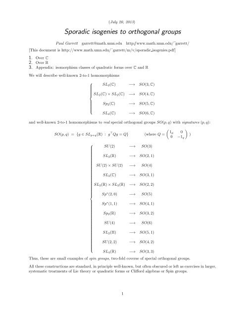
We will describe well-known 2-to-1 homomorphisms
⎧
SL 2 (C) −→ SO(3, C)
⎪⎨ SL 2 (C) × SL 2 (C) −→ SO(4, C)
⎪⎩
Sp 2 (C) −→ SO(5, C)
SL 4 (C) −→ SO(6, C)
and well-known 2-to-1 homomorphisms to real special orthogonal groups SO(p, q) with signatures (p, q):
SO(p, q) = {g ∈ SL p+q (R) : g ⊤ Qg = Q} (where Q =
⎧
SU(2) −→ SO(3)
SL 2 (R) −→ SO(2, 1)
SU(2) × SU(2) −→ SO(4)
SL 2 (C) −→ SO(3, 1)
SL 2 (R) × SL 2 (R) −→ SO(2, 2)
( )
1p 0
)
0 −1 q
⎪⎨
Sp ∗ (2, 0) −→ SO(5)
⎪⎩
Sp ∗ (1, 1) −→ SO(4, 1)
Sp 2 (R) −→ SO(3, 2)
SU(4) −→ SO(6)
SL 2 (H) −→ SO(5, 1)
SU(2, 2) −→ SO(4, 2)
SL 4 (R) −→ SO(3, 3)
Thus, these are small examples of spin groups, two-fold coverse of special orthogonal groups.
All these constructions are standard, in principle well-known, but often obscured or left as exercises in larger,
systematic treatments of Lie theory or quadratic forms or Clifford algebras or Spin groups.
1

Paul Garrett: Sporadic isogenies to orthogonal groups (July 20, 2013)
1. Over C
[1.1] SL 2 (C) → SO(3, C) The space V of 2-by-2 complex matrices with trace 0, has symmetric bilinear
form 〈x, y〉 = tr(xy). The action of SL 2 (C) on V by g · x = gxg −1 preserves 〈, 〉:
〈g · x, g · y〉 = tr(gxg −1 · gyg −1 ) = tr(g · xy · g −1 ) = tr(xy) = 〈x, y〉
An orthogonal basis is (
1 0
0 −1
) (
0 1
1 0
) (
0
)
1
−1 0
with 〈, 〉 values 2, 2, −2, demonstrating non-degeneracy. Thus, SL 2 (C) maps to a copy of SO(3, C). The
kernel is just {±1}.
[1.2] SL 2 (C) × SL 2 (C) → SO(4, C) Let V = M 2 (C) be 2-by-2 complex matrices, with (g, h) ∈
SL 2 (C) × SL 2 (C) acting by (g, h) · x = gxh −1 . Give V the bilinear form
( )
〈x, y〉 = tr(x · wy ⊤ w −1 0 −1
) (where w = )
1 0
It is symmetric because trace is invariant under transpose, and because w −1 = −w. For g ∈ SL 2 (C),
g −1 = wg ⊤ w −1 , and the pairing is invariant under the group action:
tr(gxh −1 · w(gyh −1 ) ⊤ w −1 ) = tr(gxh −1 · w(h −1 ) ⊤ w −1 · wy ⊤ w −1 · wg ⊤ w −1 )
= tr(gxh −1 · h · wy ⊤ w −1 · g −1 ) = tr(g · xwy ⊤ w −1 · g −1 ) = tr(xwy ⊤ w −1 )
Computing
( ) ( )
a b a
′
b
〈 ,
′ ( ( ) ( )
a b d
′
−b
c d c ′ d ′ 〉 = tr
′ ) ( )
ad
c d −c ′ a ′ = tr
′ − bc ′ ∗
∗ da ′ − cb ′
an orthogonal basis is readily found: for example, [1]
(
1
)
0
(
1 0
0 1 0 −1
) (
0 1
−1 0
) (
0
)
1
1 0
= ad ′ − bc ′ − cb ′ + da ′
with 〈, 〉 values 2, −2, 2, −2, demonstrating non-degeneracy.
SO(4, C).
Thus, SL 2 (C) × SL 2 (C) maps to a copy of
[1.3] Sp 2 (C) → SO(5, C) The symplectic group [2] is
⎛
⎞
0 0 −1 0
Sp 2 (C) = {g ∈ GL 4 (C) : g ⊤ ⎜ 0 0 0 −1 ⎟
Jg = J} (with J = ⎝
⎠)
1 0 0 0
0 1 0 0
[1]
One can also observe from this expression that the bilinear form is a sum of two hyperbolic planes, thus giving
signature (2, 2) without further computation.
[2]
In some conventions, the subscript is made to be the size, so what we call Sp 2 here might be called Sp 4 elsewhere.
2

Paul Garrett: Sporadic isogenies to orthogonal groups (July 20, 2013)
Write g σ = Jg ⊤ J −1 , so the condition can be rewritten as g σ g = 1 2 . The C-vectorspace V will be a subspace
of the space M 4 (C) of 4-by-4 complex matrices. Let 〈x, y〉 = tr(xy) on M 4 (C). Let Sp 2 (C) act on M 4 (C) by
g · x = gxg σ . This action respects 〈, 〉:
〈g · x, g · y〉 = tr(gxg σ · gyg σ ) = tr(g · xy · g −1 ) = tr(xy) = 〈x, y〉
Since 1 4 = g σ g = g · 1 4 · g σ , the action has fixed-point 1 4 , and the subspace
V = {x ∈ M 4 (C) : x σ = x and 〈x, 1 4 〉 = 0}
is stable under the action. In 2-by-2 blocks, the condition x σ = x is
( )
a b
=
c d
(
0 −1
1 0
) (
a b
c d
) ⊤ (
0
)
1
−1 0
=
( ) ( ) ( )
0 −1 a ⊤ c ⊤ 0 1
1 0 b ⊤ d ⊤ −1 0
=
( )
d
⊤
−b ⊤
−c ⊤ a ⊤
Thus, d = a ⊤ and b, c are skew-symmetric. The condition 〈x, 1 4 〉 = 0 requires tr(a) = 0. Thus, dim C V = 5.
To check that 〈, 〉 is non-degenerate on V , identify an orthogonal basis, such as
⎛
1 0
⎜ 0
⎝
−1
⎞
⎟
⎠
1 0
0 −1
⎛
0 1
⎜ 1
⎝
0
where empty positions are 0.
⎞
⎟
⎠
0 1
1 0
⎛
0 1
⎜ −1 0
⎝
⎞
⎟
⎠
0 −1
1 0
⎛
⎜
⎝
0 1
−1 0
⎞
0 1
−1 0 ⎟
⎠
⎛
⎜
⎝
0 −1
1 0
⎞
0 1
−1 0 ⎟
⎠
[1.4] SL 4 (C) → SO(6, C) Let SL 4 (C) act in the natural way on the six-dimensional vectorspace
V = ∧2 C 4 , namely, g · (v ∧ w) = gv ∧ gw. Let e 1 , e 2 , e 3 , e 4 be the standard basis of C 4 , and define [3] 〈, 〉 on
V by
x ∧ y = 〈x, y〉 · e 1 ∧ e 2 ∧ e 3 ∧ e 4 (with x, y ∈ ∧2 C 4 )
This form is symmetric because an even number of transpositions reverses the arguments:
(x ∧ y) ∧ (z ∧ w) = −x ∧ z ∧ y ∧ w = x ∧ z ∧ w ∧ y = −z ∧ x ∧ w ∧ y
= −z ∧ x ∧ w ∧ y = (z ∧ w) ∧ (x ∧ y) (for x, y, z, y ∈ C 4 )
The form is invariant under the action because
〈
g · (x ∧ y), g · (z ∧ w)
〉
· e1 ∧ e 2 ∧ e 3 ∧ e 4 = gx ∧ gy ∧ gz ∧ gw = det g · x ∧ y ∧ z ∧ w
To check non-degeneracy, observe
= det g · 〈x
∧ y, z ∧ w 〉 · e 1 ∧ e 2 ∧ e 3 ∧ e 4
〈
e1 ∧ e 2 , e 3 ∧ e 4
〉
= 1
〈
e1 ∧ e 3 , e 2 ∧ e 4
〉
= −1
〈
e1 ∧ e 4 , e 2 ∧ e 3
〉
= 1
while 〈e i ∧ e j , e k ∧ e l 〉 = 0 when {i, j} ∩ {k, l} ≠ φ. Thus, an orthogonal basis is
with 〈, 〉 values ±2, ∓2, ±2.
(e 1 ∧ e 2 ) ± (e 3 ∧ e 4 ) (e 1 ∧ e 3 ) ± (e 2 ∧ e 4 ) (e 1 ∧ e 4 ) ± (e 2 ∧ e 3 )
[3]
It is not necessary to choose a basis for C 4 , only to choose a basis for ∧ 4 C 4 .
3

Paul Garrett: Sporadic isogenies to orthogonal groups (July 20, 2013)
2. Over R
Each homomorphism of complex groups gives rise to several homomorphisms of real groups.
[2.1] SU(2) → SO(3) The standard special unitary group SU(2) is
SU(2) = {g ∈ SL 2 (C) : g ∗ g = 1 2 }
(where g ∗ is g-conjugate-transpose)
The space V of 2-by-2 skew-hermitian complex matrices with trace 0 has symmetric real-valued real-bilinear
form 〈x, y〉 = Re(tr(xy)). An orthogonal basis is
(
i 0
0 −i
) (
0 1
−1 0
) (
0
)
i
i 0
Each has value −2 for 〈, 〉, so the signature of 〈, 〉 on V is (0, 3). The action of SU(2) on V by g · x = gxg ∗
preserves 〈, 〉, because
tr(gxg ∗ · gyg ∗ ) = tr(g · xy · g −1 ) = tr(xy)
Thus, SU(2) maps to a copy of SO(3). The kernel is just {±1}.
[2.2] SL 2 (R) → SO(2, 1) The space V of 2-by-2 real matrices with trace 0, with symmetric bilinear
form 〈x, y〉 = tr(xy), has orthogonal basis
(
1 0
0 −1
) (
0 1
1 0
) (
0
)
1
−1 0
The values of 〈, 〉 are respectively 2, 2, −2, giving signature (2, 1). The action of SL 2 (R) on V by g·x = gxg −1
preserves 〈, 〉:
〈g · x, g · y〉 = tr(gxg −1 · gyg −1 ) = tr(g · xy · g −1 ) = tr(xy) = 〈x, y〉
Thus, SL 2 (R) maps to a copy of SO(2, 1). The kernel is just {±1}.
[2.3] SU(2) × SU(2) → SO(4) Let [4]
( )
V = {complex 2-by-2 matrices x : x ∗ = wx ⊤ w −1 0 −1
} (with w = )
1 0
( )
α β
= {2-by-2 complex matrices of the form
with α, β ∈ C}
−β α
Let (g, h) ∈ SU(2) × SU(2) act by (g, h) · x = gxh ∗ . Give V the bilinear form
〈x, y〉 = Re(tr(xy ∗ ))
[4]
It is not a coincidence that the vectorspace is a standard model of the Hamiltonian quaternions:
( )
a + bi c + di
a + bi + cj + dk −→
c − di a − bi
4

Paul Garrett: Sporadic isogenies to orthogonal groups (July 20, 2013)
For g ∈ SU(2) ⊂ SL 2 (R), g −1 = wg ⊤ w −1 , giving the stabilization of V by the group action:
w(gxh ∗ ) ⊤ w −1 = w(h ∗ ) ⊤ w −1 · wx ⊤ w −1 · wg ⊤ w −1 = (h ∗ ) −1 x ∗ g −1 = hx ∗ g ∗ = (gxh ∗ ) ∗
The pairing is invariant under the group action:
tr(gxh −1 · w(gyh −1 ) ⊤ w −1 ) = tr(gxh −1 · w(h −1 ) ⊤ w −1 · wy ⊤ w −1 · wg ⊤ w −1 )
= tr(gxh −1 · h · wy ⊤ w −1 · g −1 ) = tr(g · xwy ⊤ w −1 · g −1 ) = tr(xwy ⊤ w −1 )
Computing
( )
α β
〈
,
−β α
(
α β
−β α
)
〉 = tr
an orthogonal basis is readily found: for example,
(
1
)
0
(
i 0
0 1 0 −i
with 〈, 〉 values 2, 2, 2, 2.
( ( ) (
α β α −β
−β α β α
) (
0 i
i 0
) ) ( )
αα + ββ ∗
= tr
∗ αα + ββ
) (
0
)
1
−1 0
[2.4] SL 2 (C) → SO(3, 1) Again with
( )
V = {complex 2-by-2 matrices x : x ∗ = wx ⊤ w −1 0 −1
} (with w = )
1 0
( )
α β
= {2-by-2 complex matrices of the form
with α, β ∈ C}
−β α
use the R-bilinear R-valued form 〈x, y〉 = Re(tr(xy)), where the overline denotes entry-wise complex
conjugation. An orthogonal basis is
(
1
)
0
(
i
)
0
(
0
)
i
(
0
)
1
0 1 0 −i
i 0 −1 0
with 〈, 〉 values 2, 2, 2, −2. Thus, the signature of 〈, 〉 is 3, 1. The action g · x = gxg −1 preserves the bilinear
form 〈x, y〉 = Re(tr(xy)) on the larger R-vectorspace of all complex 2-by-2 matrices, since
tr(gxg −1 · gyg −1 ) = tr(gxg −1 · gyg −1 ) = tr(g · xy · g −1 ) = tr(xy)
To check that SL 2 (C) stabilizes V , recall that g −1 = wg ⊤ w −1 for g ∈ SL 2 (C). For y ∈ V , by design,
(gyg −1 ) ∗ = (g −1 ) ∗ y ∗ g ∗ = (g ⊤ ) −1 · wyw −1 · g ⊤ = w(g ⊤ ) ⊤ w −1 · wyw −1 · wg −1 w −1
= wgw −1 · wyw −1 · w(g −1 )w −1 = w(gyg −1 )w −1
so SL 2 (C) stabilizes V , and maps to a copy of SO(3, 1). The kernel is just {±1}.
[2.5] SL 2 (R) × SL 2 (R) → SO(2, 2) Let V be 2-by-2 real matrices, with (g, h) ∈ SL 2 (R) × SL 2 (R)
acting by (g, h) · x = gxh −1 . Give V the bilinear form
( )
〈x, y〉 = tr(x · wy ⊤ w −1 0 −1
) (where w = )
1 0
5

Paul Garrett: Sporadic isogenies to orthogonal groups (July 20, 2013)
It is symmetric because trace is invariant under transpose, and because w −1 = −w. For g ∈ SL 2 (R),
g −1 = wg ⊤ w −1 , and the pairing is invariant under the group action:
tr(gxh −1 · w(gyh −1 ) ⊤ w −1 ) = tr(gxh −1 · w(h −1 ) ⊤ w −1 · wy ⊤ w −1 · wg ⊤ w −1 )
= tr(gxh −1 · h · wy ⊤ w −1 · g −1 ) = tr(g · xwy ⊤ w −1 · g −1 ) = tr(xwy ⊤ w −1 )
Computing
( ) ( )
a b a
′
b
〈 ,
′ ( ( ) ( )
a b d
′
−b
c d c ′ d ′ 〉 = tr
′ ) ( )
ad
c d −c ′ a ′ = tr
′ − bc ′ ∗
∗ da ′ − cb ′
an orthogonal basis is readily found: for example, [5]
(
1 0
0 1
) (
1 0
0 −1
with 〈, 〉 values 2, −2, 2, −2, giving the desired signature.
) (
0 1
−1 0
) (
0
)
1
1 0
= ad ′ − bc ′ − cb ′ + da ′
[2.6] Sp ∗ (2, 0) → SO(5) Let H be the Hamiltonian quaternions. One model of G = Sp ∗ 2 = Sp ∗ (2, 0) is
Sp ∗ (2, 0) = {g ∈ GL 2 (H) : g ∗ g = 1 2 }
where g ∗ = g ⊤ with entry-wise quaternion conjugation. The R-vectorspace V will be a subspace of the space
M 2 (H) of 2-by-2 matrices with entries in H. Let λ be the reduced trace
( )
α β
λ
γ δ
= 1 2
· (α + α + δ + δ)
and on M 2 (H) let 〈x, y〉 = λ(xy). Let G act on M 2 (H) by g · x = gxg ∗ . This action respects 〈, 〉:
Thus,
〈g · x, g · y〉 = λ(gxg ∗ · gyg ∗ ) = λ(g · xy · g −1 ) = λ(xy)
( )
V = {y ∈ M 2 (H) : y ∗ a β
= y and 〈y, 1 2 〉 = 0} = {
: a ∈ R, β ∈ H}
β −a
is stable under this action, and dim R V = 5. An orthogonal basis is
(
1 0
0 1
) (
0 1
1 0
) (
0 i
−i 0
with values 2, 2, 2, 2, 2, giving the desired signature.
) (
0 j
−j 0
) (
0
)
k
−k 0
[2.7] Sp ∗ (1, 1) → SO(4, 1) One model of G = Sp ∗ (1, 1) is
Sp ∗ (1, 1) = {g ∈ GL 2 (H) : g ∗ Sg = S} (with S =
( )
0 1
)
1 0
[5]
One can also observe from this expression that the bilinear form is a sum of two hyperbolic planes, thus giving
signature (2, 2) without further computation.
6

Paul Garrett: Sporadic isogenies to orthogonal groups (July 20, 2013)
where g ∗ = g ⊤ with entry-wise quaternion conjugation. Let g σ = Sg ∗ S −1 , so the defining condition is
g σ g = 1 2 . The R-vectorspace V will be a subspace of the space M 2 (H) of 2-by-2 matrices with entries in H.
Let 〈x, y〉 = λ(xy). Let G act on M 2 (H) by g · x = gxg σ . This action respects 〈, 〉:
〈g · x, g · y〉 = λ(gxg σ · gyg σ ) = λ(g · xy · g σ ) = λ(g · xy · g −1 ) = λ(xy) = 〈x, y〉
The R-vectorspace is
( )
V = {x ∈ M 2 (H) : x σ α b
= x and 〈x, S〉 = 0} = {
−b α
: α ∈ H, b ∈ R}
and is stable under the action, and dim R V = 5. An orthogonal basis is
(
1
)
0
(
i
)
0
(
j
)
0
(
k
)
0
(
0
)
1
0 1 0 −i 0 −j 0 −k −1 0
with values 2, −2, −2, −2, −2, giving the desired signature.
[2.8] Sp 2 (R) → SO(3, 2) The symplectic group is
⎛
⎞
0 0 −1 0
Sp 2 (R) = {g ∈ GL 4 (R) : g ⊤ ⎜ 0 0 0 −1 ⎟
Jg = J} (with J = ⎝
⎠)
1 0 0 0
0 1 0 0
Write g σ = Jg ⊤ J −1 , so the condition can be rewritten as g σ g = 1 2 . The R-vectorspace V will be a subspace
of the space M 4 (R) of 4-by-4 real matrices. Let 〈x, y〉 = tr(xy). Let Sp 2 (R) act on M 4 (R) by g · x = gxg σ .
This action respects 〈, 〉:
〈g · x, g · y〉 = tr(gxg σ · gyg σ ) = tr(g · xy · g −1 ) = tr(xy) = 〈x, y〉
Since 1 4 = g σ g = g 1 4 g σ , the action has fixed-point 1 4 , and the subspace
V = {x ∈ M 4 (R) : x σ = x and 〈x, 1 4 〉 = 0}
is stable under the action. In 2-by-2 blocks, the condition x σ = x is
( )
a b
=
c d
(
0 −1
1 0
) (
a b
c d
) ⊤ (
0
)
1
−1 0
=
( ) ( ) ( )
0 −1 a ⊤ c ⊤ 0 1
1 0 b ⊤ d ⊤ −1 0
=
( )
d
⊤
−b ⊤
−c ⊤ a ⊤
Thus, d = a ⊤ and b, c are skew-symmetric. The condition 〈x, 1 4 〉 = 0 requires that tr(a) = 0. Thus,
dim R V = 5. The easily observed orthogonal basis
⎛
1 0
⎜ 0
⎝
−1
⎞
⎟
⎠
1 0
0 −1
⎛
0 1
⎜ 1
⎝
0
⎞
⎟
⎠
0 1
1 0
⎛
0 1
⎜ −1 0
⎝
has 〈, 〉 values 4, 4, −4, −4, 4, giving signature 3, 2.
⎞
⎟
⎠
0 −1
1 0
⎛
⎜
⎝
0 1
−1 0
⎞
0 1
−1 0 ⎟
⎠
⎛
⎜
⎝
0 −1
1 0
⎞
0 1
−1 0 ⎟
⎠
[2.9] SU(4) → SO(6) Let e 1 , e 2 , e 3 , e 4 be the standard basis for C 4 . Give ∧2 C 4 the C-valued SL 4 (C)-
invariant symmetric form
〈 〉
x ∧ y, z ∧ w · e1 ∧ e 2 ∧ e 3 ∧ e 4 = x ∧ y ∧ z ∧ w (for x, y, z, w ∈ C 4 )
7

Paul Garrett: Sporadic isogenies to orthogonal groups (July 20, 2013)
A six-dimensional R-subspace of ∧2 C 4 stable under SU(4) will be identified as the fixed vectors of an
C-conjugate-linear isomorphism J : C 4 → C 4 commuting with SU(4), on which 〈, 〉 takes real values.
To make such J, use the positive-definite hermitian form (x, y) = y ∗ x on C 4 invariant under SU(4),
giving a C-conjugate-linear isomorphism C 4 → (C 4 ) ∗ by x → (y → (y, x)), which induces ∧2 C 4 →
∧ 2
(C 4∗ ) ≈ ( ∧2 C 4 ) ∗ . At the same time, the non-degenerate form 〈, 〉 on ∧2 C 4 gives a C-linear isomorphism
∧ 2
C 4 → ∧2 C 4 by v → (w → 〈w, v〉). Combining these,
J
∧ 2
C 4
〈,〉
( ∧2 C 4 ) ∗ ≈
∧ 2
(C 4∗ )
(,)∧(,)
∧ 2
C 4
with the right-to-left arrow a C-conjugate-linear isomorphism, gives a C-conjugate-linear isomorphism J of
∧ 2
C 4 to itself. Since SU(4) respects both 〈, 〉 and (, ), the map J commutes with SU(4). This is noted
element-wise below.
We can track basis elements e k ∧e l under J. Since functionals 〈−, e 1 ∧e 2 〉 and (−, e 3 )∧(−, e 4 ) both compute
the e 3 ∧ e 4 component of ∑ k

Paul Garrett: Sporadic isogenies to orthogonal groups (July 20, 2013)
[2.10] SL 2 (H) → SO(5, 1) Imbed H ⊂ M 2 (C) by
( )
a + bi c + dj
a + bi + cj + dk −→
−c + di a − bi
(with a, b, c, d ∈ R)
Note the characterization
H = {x ∈ M 2 (C) : x = wxw −1 } (with w =
( )
0 −1
)
1 0
Thus, identify
⎛
0 −1
SL 2 (H) = {g ∈ SL 4 (C) : g = W gW −1 }
⎜ 1
(where W = ⎝
0
⎞
⎟
⎠)
0 −1
1 0
where g → g is entry-wise conjugation. Let e 1 , e 2 , e 3 , e 4 be the standard basis for C 4 , and give ∧2 C 4 the
C-valued SL 4 (C)-invariant symmetric form
〈
x ∧ y, z ∧ w
〉
· e1 ∧ e 2 ∧ e 3 ∧ e 4 = x ∧ y ∧ z ∧ w (for x, y, z, w ∈ C 4 )
A six-dimensional R-subspace of ∧2 C 4 stable under SU(4) will be identified as the fixed vectors of an
C-conjugate-linear isomorphism J : C 4 → C 4 commuting with SL 2 (H), on which 〈, 〉 takes real values.
Define conjugate-linear J : ∧2 C 4 → ∧2 C 4 by
J(x ∧ y) = W x ∧ W y
By design, J commutes with the action of g ∈ SL 2 (H):
g · J(x ∧ y) = gW x ∧ gW y = W W −1 gW x ∧ W W −1 gW y = W gx ∧ W gy = J(g · x ∧ y)
The effect of J on e k ∧ e l and ie k ∧ e l is readily computed, since W e 1 = e 2 , W e 2 = −e 1 , W e 3 = e 4 , and
W e 4 = −e 3 :
J(e 1 ∧ e 2 ) = −e 2 ∧ e 1 = e 1 ∧ e 2 J(e 3 ∧ e 4 ) = −e 4 ∧ e 3 = e 3 ∧ e 4
while
and
J(e 1 ∧ e 3 ) = e 2 ∧ e 4 J(e 2 ∧ e 4 ) = −e 1 ∧ −e 3 = e 1 ∧ e 3
J(e 1 ∧ e 4 ) = e 2 ∧ −e 3 = −e 2 ∧ e 3 J(e 2 ∧ e 3 ) = −e 1 ∧ e 4
Visibly, J 2 = 1 on these vectors. Since J is conjugate-linear, we have J 2 = 1. An orthogonal basis for +1
eigenvectors is
e 1 ∧e 2 +e 3 ∧e 4 e 1 ∧e 2 −e 3 ∧e 4 e 1 ∧e 3 +e 2 ∧e 4 ie 1 ∧e 3 −ie 2 ∧e 4 e 1 ∧e 4 −e 2 ∧e 3 ie 1 ∧e 4 +ie 2 ∧e 3
with 〈, 〉 values 2, −2, −2, −2, −2, −2.
[2.11] SU(2, 2) → SO(4, 2) One model of SU(2, 2) is
⎛
1
SU(2, 2) = {g ∈ SL 4 (C) : g ∗ ⎜
Sg = S} (where S = ⎝
1
−1
−1
⎞
⎟
⎠)
9

Paul Garrett: Sporadic isogenies to orthogonal groups (July 20, 2013)
Again, with e 1 , e 2 , e 3 , e 4 the standard basis for C 4 , give ∧2 C 4 the C-valued symmetric form
〈
x ∧ y, z ∧ w
〉
· e1 ∧ e 2 ∧ e 3 ∧ e 4 = x ∧ y ∧ z ∧ w (for x, y, z, w ∈ C 4 )
A six-dimensional R-subspace of ∧2 C 4 stable under SU(2, 2) will be identified as the fixed vectors of an
C-conjugate-linear isomorphism J : C 4 → C 4 commuting with SU(2, 2), and on which 〈, 〉 takes real values.
Use the non-degenerate hermitian form
(x, y) = y ∗ Sx
on C 4 invariant under SU(2, 2), giving C-conjugate-linear isomorphism C 4 → (C 4 ) ∗ by x → (y → (y, x)),
which induces ∧2 C 4 → ∧2 (C 4∗ ) ≈ ( ∧2 C 4 ) ∗ . At the same time, the non-degenerate form 〈, 〉 on ∧2 C 4 gives
a C-linear isomorphism ∧2 C 4 → ∧2 C 4 by v → (w → 〈w, v〉). Combining these,
J
∧ 2
C 4
〈,〉
( ∧2 C 4 ) ∗ ≈
∧ 2
(C 4∗ )
(,)∧(,)
∧ 2
C 4
with the right-to-left arrow a C-conjugate-linear isomorphism, gives a C-conjugate-linear isomorphism J of
∧ 2
C 4 to itself. Since SU(2) respects both 〈, 〉 and (, ), the map J commutes with SU(2). This is noted
element-wise below. It is important to check that J 2 = 1.
Tracking e k ∧ e l and ie k ∧ e l under J is nearly identical to that for SU(4), with important sign flips.
Functionals 〈−, e 1 ∧e 2 〉 and (−, e 3 )∧(−, e 4 ) both compute the e 3 ∧e 4 component of ∑ k

Paul Garrett: Sporadic isogenies to orthogonal groups (July 20, 2013)
The last four have sign flips in comparison to the analogous basis for SU(4),
2, 2, −2, −2, −2, −2.
giving 〈, 〉 values
[2.12] Why not SU(3, 1)? One model of SU(3, 1) is
⎛
1
SU(3, 1) = {g ∈ SL 4 (C) : g ∗ ⎜
Sg = S} (where S = ⎝
1
1
−1
⎞
⎟
⎠)
We could attempt the same procedure for SU(3, 1) as for SU(4), SL 2 (H), and SU(2, 2), by arranging a
conjugate-linear map J on ∧2 C 4 and commuting with SU(3, 1), and hoping that the SL 4 (C)-invariant C-
valued form 〈, 〉 on ∧2 C 4 is real-valued on J-eigenspaces. Indeed, the same diagrammatic description of J
produces a conjugate-linear map J commuting with SU(3, 1), so SU(3, 1) stabilizes eigenspaces of J.
However, J 2 = −1, not +1, on C 4 :
The functionals 〈−, e 1 ∧ e 2 〉 and (−1)(−, e 3 ) ∧ (−, e 4 ) both compute the e 3 ∧ e 4 component, so
J(e 1 ∧ e 2 ) = −e 3 ∧ e 4
while 〈−, e 3 ∧ e 4 〉 and (−, e 1 ) ∧ (−, e 2 ) both compute the e 1 ∧ e 2 component, so
J(e 3 ∧ e 4 ) = e 1 ∧ e 2
Similarly, (−1)〈−, e 1 ∧ e 3 〉 and (−1)(−, e 2 ) ∧ (−, e 4 ) both compute the e 2 ∧ e 4 component, so
J(e 1 ∧ e 3 ) = e 2 ∧ e 4
while (−1)〈−, e 2 ∧ e 4 〉 and (−, e 1 ) ∧ (−, e 3 ) both compute the e 1 ∧ e 3 component, giving
J(e 2 ∧ e 4 ) = −e 1 ∧ e 3
Functionals 〈−, e 1 ∧ e 4 〉 and (−, e 2 ) ∧ (−, e 3 ) both compute the e 2 ∧ e 3 component, so
J(e 1 ∧ e 4 ) = e 3 ∧ e 3
while 〈−, e 2 ∧ e 3 〉 and (−1)(−, e 1 ) ∧ (−, e 4 ) both compute the e 1 ∧ e 4 component, so
J(e 2 ∧ e 3 ) = −e 1 ∧ e 4
Thus, J 2 = −1, not +1, on ∧2 C 4 . Thus, the only possible eigenvalues are ±i.
Nevertheless, any J-eigenspace inside the R-vectorspace ∧2 C 4 is stabilized by SU(3, 1). But the conjugatelinearity
of J shows that there cannot be ±i-eigenvalues in ∧2 C 4 : if Jv = iv, then
−v = J 2 v = J(iv) = −iJv = (−i)iv = v
Thus, this device has failed to produce SU(3, 1)-stable proper R-subspaces of ∧2 C 4 .
11

Paul Garrett: Sporadic isogenies to orthogonal groups (July 20, 2013)
3. Appendix: isomorphism classes of forms over C and R
For convenience, we recall a classification over C and over R: as elaborated below, dimension is the only
invariant of non-degenerate symmetric bilinear forms over C, and signature is the only invariant over R.
A vector space V with a symmetric bilinear form over a field is non-degenerate when, for every v ≠ 0 in V ,
there is w ∈ V such that 〈v, w〉 ≠ 0.
The corresponding orthogonal group is the isometry group
{g ∈ Aut k (V ) : 〈gv, gw〉 = 〈v, w〉, for all v, w ∈ V }
A basis {v i } is orthogonal when 〈v i , v j 〉 = 0 for i ≠ j.
[3.1] Non-degenerate forms over C classified by dimension We claim that for a non-degenerate
symmetric bilinear C-valued form 〈, 〉 on a finite-dimensional C-vectorspace V , there is an orthogonal basis
v 1 , . . . , v n such that 〈v i , v i 〉 = 1 for all i.
Given v ≠ 0 in V , when 〈v, v〉 ≠ 0. Replace v by v 1 = v/ √ 〈v, v〉 with either square root, to arrange
〈v 1 , v 1 〉 = 1. When 〈v, v〉 = 0, use non-degeneracy to obtain w such that 〈v, w〉 ≠ 0. In case 〈w, w〉 ≠ 0, we
are in the first case, and if 〈w, w〉 = 0, then 〈v + w, v + w〉 = 2 ≠ 0, and again we are back to the first case.
That is, there is a vector with 〈v, v〉 = 1.
To complete the induction argument, show that for 〈v, v〉 = 1 the orthogonal complement
v ⊥ = {w ∈ V : 〈v, w〉 = 0}
is non-degenerate. Indeed, given 0 ≠ v ′ ∈ v ⊥ , let w ∈ V such that 〈v ′ , w〉 ≠ 0. Retain this property while
adjusting w to be in v ⊥ by replacing it by w − 〈w, v〉. ///
Thus, dimension is the only isomorphism-class invariant of non-degenerate symmetric bilinear forms over C,
or over any algebraically closed field of characteristic not 2. The standard model is
O(n, C) = {g ∈ GL n (C) : g ⊤ g = 1 n }
[3.2] Non-degenerate forms over R classified by signature We claim that for non-degenerate R-valued
symmetric bilinear form 〈, 〉 on a finite-dimensional C-vectorspace V , there are non-negative integers p, q and
an orthogonal basis v 1 , . . . , v p , w 1 , . . . w q such that that 〈v i , v i 〉 = 1 for 1 ≤ i ≤ p and 〈w j , w j 〉 = −1 for
1 ≤ j ≤ q.
This is Sylvester’s law of inertia. The pair (p, q) is the signature. The standard model is
( )
O(p, q) = {g ∈ GL p+q (R) : g ⊤ 1p 0
Qg = Q} (where Q =
)
0 −1 q
Given v ≠ 0, when 〈v, v〉 ≠ 0, replacing v by v/ √ |〈v, v〉| gives 〈v, v〉 = ±1. When 〈v, v〉 = 0, there is w such
that 〈v, w〉 ≠ 0. In case 〈w, w〉 ≠ 0, we are back to the first case. When 〈w, w〉 = 0, 〈v + w, v + w〉 = 2 ≠ 0,
and again we are back to the first case.
Thus, there is v with 〈v, v〉 = ±1.
An argument nearly identical to the complex case shows that v ⊥ is non-degenerate, so and induction gives
existence of a signature.
12

Paul Garrett: Sporadic isogenies to orthogonal groups (July 20, 2013)
For uniqueness, let a totally isotropic subspace W of V be a subspace on which 〈, 〉 = 0, that is, 〈w, w ′ 〉 = 0
for all w, w ′ ∈ W . A maximal totally isotropic subspace is also called Lagrangian.
We claim that all Lagrangian subspaces W have the same dimension. Uniqueness of signature will follow
from showing this common dimension is min(p, q).
A reformulation of the definition of maximal totally isotropic is that W ⊥ is just W itself. Thus, for W ′ another
maximal totally isotropic subspace, the non-degenerate 〈, 〉 gives a non-degenerate pairing of W/(W ∩ W ′ )
and W ′ /(W ∩ W ′ ). A non-degenerate pairing between finite-dimensional vectorspaces gives an isomorphism
of each to the dual of the other, so the dimensions are equal.
Next, given a totally isotropic subspace W , there is another totally isotropic subspace W ′ such that 〈, 〉
is non-degenerate on W + W ′ . Indeed, given w 1 ∈ W , find w 1 ′ such that 〈w 1 , w 1〉 ′ ≠ 0. Without loss of
generality, 〈w 1, ′ w 1〉 ′ = 0, since otherwise replace w 1 ′ by w 1 ′ − 1 2〈w 1, ′ w 1〉 ′ · w 1 . As above, (Rw 1 + Rw 1) ′ ⊥ is
non-degenerate, and W ∩ (Rw 1 + Rw 1) ′ ⊥ is codimension 1 inside W . Thus, an induction chooses a basis
w 1, ′ . . . , w m ′ for another totally isotropic subspace W , with 〈w i , w i ′〉 = 1 for all i, and 〈w i, w j ′ 〉 = 0 for i ≠ j.
Thus, given a Lagrangian subspace W , there are corresponding w 1 , w ′ 1, . . . w m , w ′ m, and the collection w i ±w ′ i
gives an orthogonal basis for the span of W +W ′ with m positive and m negative values. Thus, min(p, q) ≥ m.
On the other hand, taking p ≥ q and orthogonal basis v 1 , . . . , v p , w 1 , . . . , w q as above, v 1 + w 1 , . . . , v q + w q
spans a totally isotropic subspace. This gives the opposite inequality, proving that min(p, q) is the (common)
dimension of Lagrangian subspaces. ///
13