Partial Differential Equations - Modelling and ... - ResearchGate
Partial Differential Equations - Modelling and ... - ResearchGate Partial Differential Equations - Modelling and ... - ResearchGate
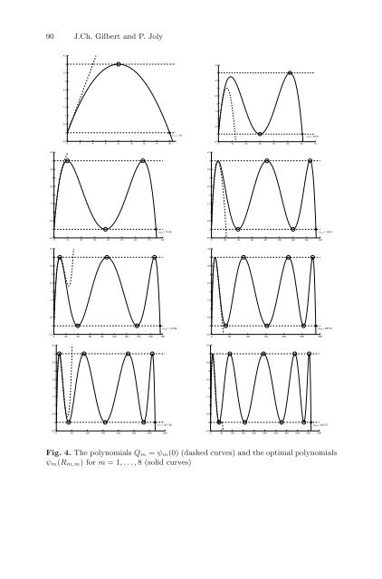
90 J.Ch. Gilbert and P. Joly 4.5 4 4.5 3.5 4 3 3.5 2.5 3 2 2.5 2 1.5 1.5 1 1 0.5 0.5 0 a 1,1 = 16 0 a 2,2 = 60.56 −0.5 0 2 4 6 8 10 12 14 16 −0.5 0 10 20 30 40 50 60 70 4.5 4.5 4 4 3.5 3.5 3 3 2.5 2.5 2 2 1.5 1.5 1 1 0.5 0.5 0 a 3,3 = 75.06 0 a 4,4 = 153.8 −0.5 0 10 20 30 40 50 60 70 80 −0.5 0 20 40 60 80 100 120 140 160 4.5 4.5 4 4 3.5 3.5 3 3 2.5 2.5 2 2 1.5 1.5 1 1 0.5 0.5 0 a 5,5 = 175.84 0 a 6,6 = 287.61 −0.5 0 20 40 60 80 100 120 140 160 180 −0.5 0 50 100 150 200 250 300 4.5 4.5 4 4 3.5 3.5 3 3 2.5 2.5 2 2 1.5 1.5 1 1 0.5 0.5 0 a 7,7 = 317.90 0 a 8,8 = 462.27 −0.5 0 50 100 150 200 250 300 350 −0.5 0 50 100 150 200 250 300 350 400 450 500 Fig. 4. The polynomials Q m = ψ m(0) (dashed curves) and the optimal polynomials ψ m(R m,m) for m =1,...,8 (solid curves)
Optimal Higher Order Time Discretizations 91 Table 2. Asymptotic behaviour of the diagonal schemes m ∆t m,m C m,m(T ) ∆t m,0 C 1,0(T ) 2α m,m m 2 π 2 1 2.00 1.00 3.24 2 3.89 1.03 3.07 3 4.33 1.39 1.69 4 6.20 1.29 1.95 5 6.63 1.51 1.43 6 8.48 1.42 1.62 7 8.91 1.57 1.31 8 10.75 1.49 1.46 ∞ 1.80 1.00 This conjecture is explored numerically in the third column of Table 2. Note that it does not distinguish between even and odd values of m, at least asymptotically. However, looking at the α m,m ’s on the diagonal of Table 1, it appears that the even values of k = m look more interesting than the odd ones. 5 Conclusion In this paper, we have analyzed the stability of higher order time discretization schemes for second order hyperbolic problems based on the modified equation approach. We have in particular proven that the upper bound for the time step (the CFL limit) remains uniformly bounded for large m (2m is the order of the scheme). On the basis of this information, we have proposed the construction of new schemes that are seen as modifications of the previous ones and are designed in order to optimize the CFL condition: this is formulated as an optimization problem in a space of polynomials of given degree. Despite some unpleasant properties (the objective function is non-convex and even discontinuous at the solution!), this problem can be fully analyzed. In particular, we prove the existence and uniqueness of the solution and give necessary and sufficient conditions of optimality. These conditions are exploited to design an algorithm for the effective numerical solution of the optimization problem. The obtained results are more than satisfactory with respect to our original objective. They suggest some conjectures that would mean that we would be able to produce schemes of arbitrary high order in time and whose computational cost would be almost independent of the order. Of course, this is a preliminary work and much has still to be done, including the following items:
- Page 47 and 48: 4 Hybridization and Condensation Mi
- Page 49 and 50: Mixed FE Methods on Polyhedral Mesh
- Page 51 and 52: is symmetric and positive definite,
- Page 53 and 54: with some coefficient α ∈ R wher
- Page 55 and 56: 44 E.J. Dean and R. Glowinski so fa
- Page 57 and 58: 46 E.J. Dean and R. Glowinski 2 A L
- Page 59 and 60: 48 E.J. Dean and R. Glowinski S:T=
- Page 61 and 62: 50 E.J. Dean and R. Glowinski minim
- Page 63 and 64: 52 E.J. Dean and R. Glowinski 6 On
- Page 65 and 66: 54 E.J. Dean and R. Glowinski Fig.
- Page 67 and 68: 56 E.J. Dean and R. Glowinski and
- Page 69 and 70: 58 E.J. Dean and R. Glowinski 7 Num
- Page 71 and 72: 60 E.J. Dean and R. Glowinski Fig.
- Page 73 and 74: 62 E.J. Dean and R. Glowinski Assum
- Page 75 and 76: Higher Order Time Stepping for Seco
- Page 77 and 78: u n+1 h Optimal Higher Order Time D
- Page 79 and 80: Optimal Higher Order Time Discretiz
- Page 81 and 82: Optimal Higher Order Time Discretiz
- Page 83 and 84: Optimal Higher Order Time Discretiz
- Page 85 and 86: Optimal Higher Order Time Discretiz
- Page 87 and 88: Optimal Higher Order Time Discretiz
- Page 89 and 90: Optimal Higher Order Time Discretiz
- Page 91 and 92: Optimal Higher Order Time Discretiz
- Page 93 and 94: Optimal Higher Order Time Discretiz
- Page 95 and 96: Optimal Higher Order Time Discretiz
- Page 97: Optimal Higher Order Time Discretiz
- Page 101 and 102: Optimal Higher Order Time Discretiz
- Page 103 and 104: 96 I. Sazonov et al. To provide a p
- Page 105 and 106: 98 I. Sazonov et al. In the first s
- Page 107 and 108: 100 I. Sazonov et al. Fig. 1. An ex
- Page 109 and 110: 102 I. Sazonov et al. H z 1 exact F
- Page 111 and 112: 104 I. Sazonov et al. (a) (b) Fig.
- Page 113 and 114: 106 I. Sazonov et al. Scattering Wi
- Page 115 and 116: 108 I. Sazonov et al. 6.4 Scatterin
- Page 117 and 118: 110 I. Sazonov et al. (a) (b) Fig.
- Page 119 and 120: 112 I. Sazonov et al. [MHP96] K. Mo
- Page 121 and 122: 114 R. Sanders and A.M. Tesdall I R
- Page 123 and 124: 116 R. Sanders and A.M. Tesdall imp
- Page 125 and 126: 118 R. Sanders and A.M. Tesdall alo
- Page 127 and 128: 120 R. Sanders and A.M. Tesdall (a)
- Page 129 and 130: 122 R. Sanders and A.M. Tesdall D C
- Page 131 and 132: 124 R. Sanders and A.M. Tesdall 8.6
- Page 133 and 134: 126 R. Sanders and A.M. Tesdall 0.3
- Page 135 and 136: 128 R. Sanders and A.M. Tesdall [TR
- Page 137 and 138: 132 S. Lapin et al. Ω R γ Ω 2 Γ
- Page 139 and 140: 134 S. Lapin et al. ∫ ∂ 2 ∫
- Page 141 and 142: 136 S. Lapin et al. Ω R γ Fig. 3.
- Page 143 and 144: 138 S. Lapin et al. 4 Energy Inequa
- Page 145 and 146: 140 S. Lapin et al. 5 Numerical Exp
- Page 147 and 148: 142 S. Lapin et al. Fig. 6. Contour
90 J.Ch. Gilbert <strong>and</strong> P. Joly<br />
4.5<br />
4<br />
4.5<br />
3.5<br />
4<br />
3<br />
3.5<br />
2.5<br />
3<br />
2<br />
2.5<br />
2<br />
1.5<br />
1.5<br />
1<br />
1<br />
0.5<br />
0.5<br />
0<br />
a 1,1 = 16<br />
0<br />
a 2,2 = 60.56<br />
−0.5<br />
0 2 4 6 8 10 12 14 16<br />
−0.5<br />
0 10 20 30 40 50 60 70<br />
4.5<br />
4.5<br />
4<br />
4<br />
3.5<br />
3.5<br />
3<br />
3<br />
2.5<br />
2.5<br />
2<br />
2<br />
1.5<br />
1.5<br />
1<br />
1<br />
0.5<br />
0.5<br />
0<br />
a 3,3 = 75.06<br />
0<br />
a 4,4 = 153.8<br />
−0.5<br />
0 10 20 30 40 50 60 70 80<br />
−0.5<br />
0 20 40 60 80 100 120 140 160<br />
4.5<br />
4.5<br />
4<br />
4<br />
3.5<br />
3.5<br />
3<br />
3<br />
2.5<br />
2.5<br />
2<br />
2<br />
1.5<br />
1.5<br />
1<br />
1<br />
0.5<br />
0.5<br />
0<br />
a 5,5 = 175.84<br />
0<br />
a 6,6 = 287.61<br />
−0.5<br />
0 20 40 60 80 100 120 140 160 180<br />
−0.5<br />
0 50 100 150 200 250 300<br />
4.5<br />
4.5<br />
4<br />
4<br />
3.5<br />
3.5<br />
3<br />
3<br />
2.5<br />
2.5<br />
2<br />
2<br />
1.5<br />
1.5<br />
1<br />
1<br />
0.5<br />
0.5<br />
0<br />
a 7,7 = 317.90<br />
0<br />
a 8,8 = 462.27<br />
−0.5<br />
0 50 100 150 200 250 300 350<br />
−0.5<br />
0 50 100 150 200 250 300 350 400 450 500<br />
Fig. 4. The polynomials Q m = ψ m(0) (dashed curves) <strong>and</strong> the optimal polynomials<br />
ψ m(R m,m) for m =1,...,8 (solid curves)


