Partial Differential Equations - Modelling and ... - ResearchGate

Optimal Higher Order Time Discretizations 89
Diagonal schemes k = m
We have found interesting to have a particular look at the case k = m. First it
gives a computational effort per time step that is twice the one for the original
(2m)th order scheme, which corresponds to k = 0. The second reason is more
related to intuition: if one wants to get α m,k roughly proportional to m 2 ,
we have to control the first m maxima or minima of the optimal polynomial
ψ m (R m,k ), for which we think that we need m parameters, which corresponds
to k = m. Below, we qualify such a scheme as diagonal.
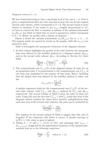
Figure 4 shows the optimal polynomials ψ m (R m,m ), for m = 1,...,8.
The tangent points are quoted by circles on the graphs, while the α m,m ’s are
quoted by dots.
Table 2 investigates the asymptotic behaviour of the diagonal schemes:
1. Its first column highlights the growth of the ratio between the maximum
time step allowed by the stability analysis in a diagonal scheme ∆t m,m
and in the second order scheme ∆t 1,0 . According to Section 2.2, there
holds
( ) 1/2
∆t m,m αm,m
=
= α1/2 m,m
. (32)
∆t 1,0 α 1,0 2
2. The computational cost C m,m (T ) of the diagonal scheme of order 2m on
an integration time T is proportional to the computational cost Cm,m 1 of
one time step multiplied by the number of time steps. Hence, assuming
that the largest time step allowed by the stability analysis is taken, one
has
C m,m (T ) ≃ C1 m,mT
.
∆t m,m
A similar expression holds for the computational cost C 1,0 (T ) of the second
order scheme, with Cm,m 1 and ∆t m,m replaced by C1,0 1 and ∆t 1,0 ,
respectively. The second column of Table 2 gives the ratio of these two
costs. Using (32) and the fact that Cm,m 1 ≃ 2mC1,0 1 (each time step of the
diagonal scheme requires 2m times more operator multiplications than
each time step of the second order scheme), the ratio can be estimated by
C m,m (T )
C 1,0 (T ) ≃
4m
α 1/2
m,m
The numbers in the second column of Table 2 suggest that this ratio is
bounded. If the conjecture (33) below is correct, it should converge to
4 √ 2/π ≃ 1.80, when m goes to infinity.
3. Taking k = m and j = ⌈m/2⌉ in (31), and assuming that α m,m ∼
2τ m,m,⌈m/2⌉ (suggested by the approximate symmetry of the optimal polynomials)
lead us to the following conjecture:
.
α m,m
m 2
→ π2
, when m →∞. (33)
2