Partial Differential Equations - Modelling and ... - ResearchGate

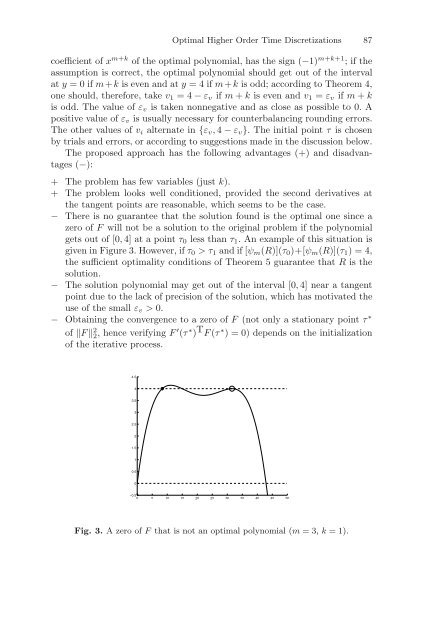
Optimal Higher Order Time Discretizations 87
coefficient of x m+k of the optimal polynomial, has the sign (−1) m+k+1 ;ifthe
assumption is correct, the optimal polynomial should get out of the interval
at y =0ifm+k is even and at y =4ifm+k is odd; according to Theorem 4,
one should, therefore, take v 1 =4− ε v if m + k is even and v 1 = ε v if m + k
is odd. The value of ε v is taken nonnegative and as close as possible to 0. A
positive value of ε v is usually necessary for counterbalancing rounding errors.
The other values of v i alternate in {ε v , 4 − ε v }. The initial point τ is chosen
by trials and errors, or according to suggestions made in the discussion below.
The proposed approach has the following advantages (+) and disadvantages
(−):
+ The problem has few variables (just k).
+ The problem looks well conditioned, provided the second derivatives at
the tangent points are reasonable, which seems to be the case.
− There is no guarantee that the solution found is the optimal one since a
zero of F will not be a solution to the original problem if the polynomial
gets out of [0, 4] at a point τ 0 less than τ 1 . An example of this situation is
given in Figure 3. However, if τ 0 >τ 1 and if [ψ m (R)](τ 0 )+[ψ m (R)](τ 1 )=4,
the sufficient optimality conditions of Theorem 5 guarantee that R is the
solution.
− The solution polynomial may get out of the interval [0, 4] near a tangent
point due to the lack of precision of the solution, which has motivated the
use of the small ε v > 0.
− Obtaining the convergence to a zero of F (not only a stationary point τ ∗
of ‖F ‖ 2 2, hence verifying F ′ (τ ∗ ) T F (τ ∗ ) = 0) depends on the initialization
of the iterative process.
4.5
4
3.5
3
2.5
2
1.5
1
0.5
0
−0.5
0 5 10 15 20 25 30 35 40 45 50
Fig. 3. AzeroofF that is not an optimal polynomial (m =3,k = 1).