Partial Differential Equations - Modelling and ... - ResearchGate

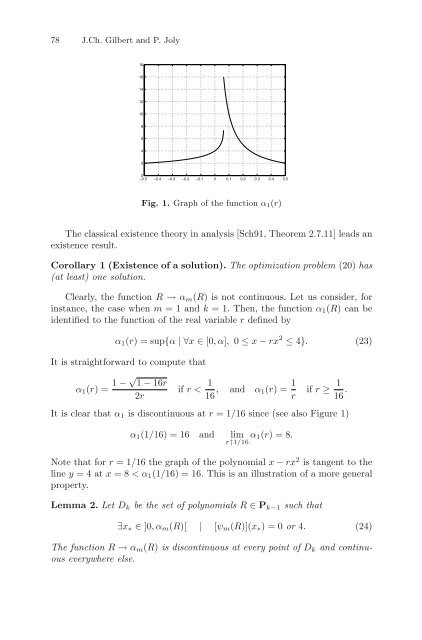
78 J.Ch. Gilbert and P. Joly
18
16
14
12
10
8
6
4
2
0
−0.5 −0.4 −0.3 −0.2 −0.1 0 0.1 0.2 0.3 0.4 0.5
Fig. 1. Graph of the function α 1(r)
The classical existence theory in analysis [Sch91, Theorem 2.7.11] leads an
existence result.
Corollary 1 (Existence of a solution). The optimization problem (20) has
(at least) one solution.
Clearly, the function R → α m (R) is not continuous. Let us consider, for
instance, the case when m =1andk = 1. Then, the function α 1 (R) can be
identified to the function of the real variable r defined by
α 1 (r) = sup{α |∀x ∈ [0,α], 0 ≤ x − rx 2 ≤ 4}. (23)
It is straightforward to compute that
α 1 (r) = 1 − √ 1 − 16r
2r
if r< 1
16 , and α 1(r) = 1 r
if r ≥ 1
16 .
It is clear that α 1 is discontinuous at r =1/16 since (see also Figure 1)
α 1 (1/16) = 16 and lim
r↑1/16 α 1(r) =8.
Note that for r =1/16 the graph of the polynomial x − rx 2 is tangent to the
line y =4atx =8