Partial Differential Equations - Modelling and ... - ResearchGate

58 E.J. Dean and R. Glowinski
7 Numerical Experiments
The least-squares based methodology discussed in the above sections has been
applied to the solution of three particular (E-MA-D) problems, with Ω =
(0, 1) 2 .Thefirst test problem can be formulated as follows (with |x| =(x 2 1 +
x 2 2) 1/2 and R ≥ √ 2):
R 2
det D 2 ψ =
(R 2 −|x| 2 ) 1 2
in Ω, ψ =(R 2 −|x| 2 ) 1 2 on Γ. (68)
The function ψ defined by ψ(x) =(R 2 −|x| 2 ) 1/2 is a solution to the problem
(68). Its graph is a piece of the sphere of center 0 and radius R. Wehave
discretized the problem (68) relying on the mixed finite element approximation
discussed in Section 6, associated to a uniform triangulation of Ω (like the
one shown on Figure 3, but finer). The uniformity of the mesh allows us
to solve the various elliptic problems encountered at each iteration of the
algorithm (57)–(64) (Algorithm 2) by fast Poisson solvers taking advantage
of the decomposition properties of the discrete analogues of the biharmonic
problems (23) and (24). To initialize the algorithm (52)–(54), we followed
Remark 6 (see Section 3) and defined ψ 0 as the solution of the discrete Poisson
problem ⎧
⎨ ψ
∫ 0 ∈ V gh ,
⎩ ∇ψ 0 · ∇vdx=2( √ f h ,v) h , ∀v ∈ V 0h
Ω
and p 0 by p 0 = D 2 h ψ 0. The algorithm (52)–(54) diverges if R = √ 2 (which
is not surprising since the corresponding ψ /∈ H 2 (Ω)). On the other hand,
for R = 2 we have a quite fast convergence as soon as τ is large enough,
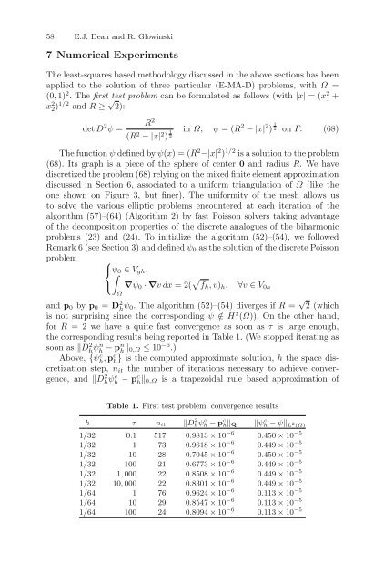
the corresponding results being reported in Table 1. (We stopped iterating as
soon as ‖Dh 2ψn h − pn h ‖ 0,Ω ≤ 10 −6 .)
Above, {ψh c, pc h
} is the computed approximate solution, h the space discretization
step, n it the number of iterations necessary to achieve convergence,
and ‖Dh 2ψc h − pc h ‖ 0,Ω is a trapezoidal rule based approximation of
Table 1. First test problem: convergence results
h τ n it ‖Dhψ 2 h c − p c h‖ Q ‖ψh c − ψ‖ L 2 (Ω)
1/32 0.1 517 0.9813 × 10 −6 0.450 × 10 −5
1/32 1 73 0.9618 × 10 −6 0.449 × 10 −5
1/32 10 28 0.7045 × 10 −6 0.450 × 10 −5
1/32 100 21 0.6773 × 10 −6 0.449 × 10 −5
1/32 1, 000 22 0.8508 × 10 −6 0.449 × 10 −5
1/32 10, 000 22 0.8301 × 10 −6 0.449 × 10 −5
1/64 1 76 0.9624 × 10 −6 0.113 × 10 −5
1/64 10 29 0.8547 × 10 −6 0.113 × 10 −5
1/64 100 24 0.8094 × 10 −6 0.113 × 10 −5