Partial Differential Equations - Modelling and ... - ResearchGate

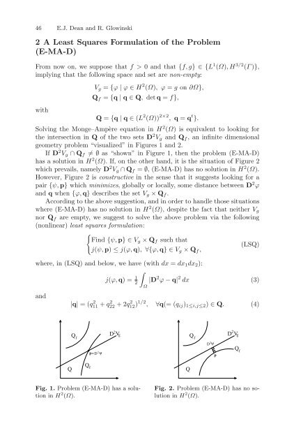
46 E.J. Dean and R. Glowinski
2 A Least Squares Formulation of the Problem
(E-MA-D)
From now on, we suppose that f>0andthat{f,g} ∈{L 1 (Ω),H 3/2 (Γ )},
implying that the following space and set are non-empty:
V g = {ϕ | ϕ ∈ H 2 (Ω), ϕ = g on ∂Ω},
Q f = {q | q ∈ Q, det q = f},
with
Q = {q | q ∈ (L 2 (Ω)) 2×2 , q = q t }.
Solving the Monge–Ampère equation in H 2 (Ω) is equivalent to looking for
the intersection in Q of the two sets D 2 V g and Q f , an infinite dimensional
geometry problem “visualized” in Figures 1 and 2.
If D 2 V g ∩ Q f ≠ ∅ as “shown” in Figure 1, then the problem (E-MA-D)
has a solution in H 2 (Ω). If, on the other hand, it is the situation of Figure 2
which prevails, namely D 2 V g ∩ Q f = ∅, (E-MA-D) has no solution in H 2 (Ω).
However, Figure 2 is constructive in the sense that it suggests looking for a
pair {ψ, p} which minimizes, globally or locally, some distance between D 2 ϕ
and q when {ϕ, q} describes the set V g × Q f .
According to the above suggestion, and in order to handle those situations
where (E-MA-D) has no solution in H 2 (Ω), despite the fact that neither V g
nor Q f are empty, we suggest to solve the above problem via the following
(nonlinear) least squares formulation:
{
Find {ψ, p} ∈V g × Q f such that
(LSQ)
j(ψ, p) ≤ j(ϕ, q), ∀{ϕ, q} ∈V g × Q f ,
where, in (LSQ) and below, we have (with dx = dx 1 dx 2 ):
∫
j(ϕ, q) = 1 2
|D 2 ϕ − q| 2 dx (3)
and
Ω
|q| =(q 2 11 + q 2 22 +2q 2 12) 1/2 , ∀q(= (q ij ) 1≤i,j≤2 ) ∈ Q. (4)
Q f
p=D 2 ψ
D 2 V g
Q
f
2
D V g
D 2 ψ
Qf
p
Q
Q f
Q
Fig. 1. Problem (E-MA-D) has a solution
in H 2 (Ω).
Fig. 2. Problem (E-MA-D) has no solution
in H 2 (Ω).