- Page 1 and 2: Partial Differential Equations
- Page 3 and 4: Partial Differential Equations Mode
- Page 5 and 6: Dedicated to Olivier Pironneau
- Page 7 and 8: VIII Preface computers has been at
- Page 9 and 10: Contents List of Contributors .....
- Page 11 and 12: List of Contributors Yves Achdou UF
- Page 13 and 14: List of Contributors XV Claude Le B
- Page 15 and 16: Discontinuous Galerkin Methods Vive
- Page 17 and 18: Discontinuous Galerkin Methods 5 2
- Page 19 and 20: Discontinuous Galerkin Methods 7 g
- Page 21 and 22: Discontinuous Galerkin Methods 9 (
- Page 23 and 24: Discontinuous Galerkin Methods 11 3
- Page 25 and 26: Discontinuous Galerkin Methods 13 3
- Page 27 and 28: Discontinuous Galerkin Methods 15 W
- Page 29 and 30: Let a h and b h denote the bilinear
- Page 31 and 32: Discontinuous Galerkin Methods 19 t
- Page 33 and 34: Discontinuous Galerkin Methods 21 l
- Page 35 and 36: Table 1. Primal DG for transport Di
- Page 37 and 38: Discontinuous Galerkin Methods 25 [
- Page 39 and 40: Mixed Finite Element Methods on Pol
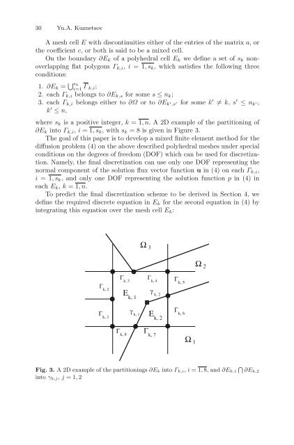
- Page 41: Mixed FE Methods on Polyhedral Mesh
- Page 45 and 46: Mixed FE Methods on Polyhedral Mesh
- Page 47 and 48: 4 Hybridization and Condensation Mi
- Page 49 and 50: Mixed FE Methods on Polyhedral Mesh
- Page 51 and 52: is symmetric and positive definite,
- Page 53 and 54: with some coefficient α ∈ R wher
- Page 55 and 56: 44 E.J. Dean and R. Glowinski so fa
- Page 57 and 58: 46 E.J. Dean and R. Glowinski 2 A L
- Page 59 and 60: 48 E.J. Dean and R. Glowinski S:T=
- Page 61 and 62: 50 E.J. Dean and R. Glowinski minim
- Page 63 and 64: 52 E.J. Dean and R. Glowinski 6 On
- Page 65 and 66: 54 E.J. Dean and R. Glowinski Fig.
- Page 67 and 68: 56 E.J. Dean and R. Glowinski and
- Page 69 and 70: 58 E.J. Dean and R. Glowinski 7 Num
- Page 71 and 72: 60 E.J. Dean and R. Glowinski Fig.
- Page 73 and 74: 62 E.J. Dean and R. Glowinski Assum
- Page 75 and 76: Higher Order Time Stepping for Seco
- Page 77 and 78: u n+1 h Optimal Higher Order Time D
- Page 79 and 80: Optimal Higher Order Time Discretiz
- Page 81 and 82: Optimal Higher Order Time Discretiz
- Page 83 and 84: Optimal Higher Order Time Discretiz
- Page 85 and 86: Optimal Higher Order Time Discretiz
- Page 87 and 88: Optimal Higher Order Time Discretiz
- Page 89 and 90: Optimal Higher Order Time Discretiz
- Page 91 and 92: Optimal Higher Order Time Discretiz
- Page 93 and 94:
Optimal Higher Order Time Discretiz
- Page 95 and 96:
Optimal Higher Order Time Discretiz
- Page 97 and 98:
Optimal Higher Order Time Discretiz
- Page 99 and 100:
Optimal Higher Order Time Discretiz
- Page 101 and 102:
Optimal Higher Order Time Discretiz
- Page 103 and 104:
96 I. Sazonov et al. To provide a p
- Page 105 and 106:
98 I. Sazonov et al. In the first s
- Page 107 and 108:
100 I. Sazonov et al. Fig. 1. An ex
- Page 109 and 110:
102 I. Sazonov et al. H z 1 exact F
- Page 111 and 112:
104 I. Sazonov et al. (a) (b) Fig.
- Page 113 and 114:
106 I. Sazonov et al. Scattering Wi
- Page 115 and 116:
108 I. Sazonov et al. 6.4 Scatterin
- Page 117 and 118:
110 I. Sazonov et al. (a) (b) Fig.
- Page 119 and 120:
112 I. Sazonov et al. [MHP96] K. Mo
- Page 121 and 122:
114 R. Sanders and A.M. Tesdall I R
- Page 123 and 124:
116 R. Sanders and A.M. Tesdall imp
- Page 125 and 126:
118 R. Sanders and A.M. Tesdall alo
- Page 127 and 128:
120 R. Sanders and A.M. Tesdall (a)
- Page 129 and 130:
122 R. Sanders and A.M. Tesdall D C
- Page 131 and 132:
124 R. Sanders and A.M. Tesdall 8.6
- Page 133 and 134:
126 R. Sanders and A.M. Tesdall 0.3
- Page 135 and 136:
128 R. Sanders and A.M. Tesdall [TR
- Page 137 and 138:
132 S. Lapin et al. Ω R γ Ω 2 Γ
- Page 139 and 140:
134 S. Lapin et al. ∫ ∂ 2 ∫
- Page 141 and 142:
136 S. Lapin et al. Ω R γ Fig. 3.
- Page 143 and 144:
138 S. Lapin et al. 4 Energy Inequa
- Page 145 and 146:
140 S. Lapin et al. 5 Numerical Exp
- Page 147 and 148:
142 S. Lapin et al. Fig. 6. Contour
- Page 149 and 150:
144 S. Lapin et al. Fig. 9. Obstacl
- Page 151 and 152:
Domain Decomposition and Electronic
- Page 153 and 154:
Domain Decomposition Approach for C
- Page 155 and 156:
Domain Decomposition Approach for C
- Page 157 and 158:
Domain Decomposition Approach for C
- Page 159 and 160:
Domain Decomposition Approach for C
- Page 161 and 162:
Domain Decomposition Approach for C
- Page 163 and 164:
Domain Decomposition Approach for C
- Page 165 and 166:
Domain Decomposition Approach for C
- Page 167 and 168:
Domain Decomposition Approach for C
- Page 169 and 170:
Numerical Analysis of a Finite Elem
- Page 171 and 172:
Numerical Analysis of a Finite Elem
- Page 173 and 174:
Numerical Analysis of a Finite Elem
- Page 175 and 176:
Numerical Analysis of a Finite Elem
- Page 177 and 178:
Numerical Analysis of a Finite Elem
- Page 179 and 180:
Numerical Analysis of a Finite Elem
- Page 181 and 182:
so that |u| 2 1,ω h ≤ 2 Numerica
- Page 183 and 184:
Numerical Analysis of a Finite Elem
- Page 185 and 186:
Numerical Analysis of a Finite Elem
- Page 187 and 188:
Numerical Analysis of a Finite Elem
- Page 189 and 190:
188 A. Bonito et al. of the model a
- Page 191 and 192:
190 A. Bonito et al. Fig. 1. The sp
- Page 193 and 194:
192 A. Bonito et al. 3 1 16 4 1 1 1
- Page 195 and 196:
194 A. Bonito et al. ∫ v n+1 h
- Page 197 and 198:
196 A. Bonito et al. −pn +2µD(v)
- Page 199 and 200:
198 A. Bonito et al. each of its pa
- Page 201 and 202:
200 A. Bonito et al. The normal vec
- Page 203 and 204:
202 A. Bonito et al. with initial c
- Page 205 and 206:
204 A. Bonito et al. Fig. 8. Jet bu
- Page 207 and 208:
206 A. Bonito et al. References [AM
- Page 209 and 210:
208 A. Bonito et al. [Set96] J. A.
- Page 211 and 212:
210 J. Hao et al. due to shear flow
- Page 213 and 214:
212 J. Hao et al. The backward reac
- Page 215 and 216:
214 J. Hao et al. where u and p den
- Page 217 and 218:
216 J. Hao et al. * * * * * * * * *
- Page 219 and 220:
218 J. Hao et al. and solve for V n
- Page 221 and 222:
220 J. Hao et al. Table 2. The calc
- Page 223 and 224:
222 J. Hao et al. References [ASS80
- Page 225 and 226:
Computing the Eigenvalues of the La
- Page 227 and 228:
Eigenvalues of the Laplace-Beltrami
- Page 229 and 230:
Eigenvalues of the Laplace-Beltrami
- Page 231 and 232:
Eigenvalues of the Laplace-Beltrami
- Page 233 and 234:
A Fixed Domain Approach in Shape Op
- Page 235 and 236:
Shape Optimization Problems with Ne
- Page 237 and 238:
Shape Optimization Problems with Ne
- Page 239 and 240:
Shape Optimization Problems with Ne
- Page 241 and 242:
Shape Optimization Problems with Ne
- Page 243 and 244:
Reduced-Order Modelling of Dispersi
- Page 245 and 246:
Reduced-Order Modelling of Dispersi
- Page 247 and 248:
Reduced-Order Modelling of Dispersi
- Page 249 and 250:
Reduced-Order Modelling of Dispersi
- Page 251 and 252:
Reduced-Order Modelling of Dispersi
- Page 253 and 254:
Reduced-Order Modelling of Dispersi
- Page 255 and 256:
Calibration of Lévy Processes with
- Page 257 and 258:
Calibration of Lévy Processes with
- Page 259 and 260:
Calibration of Lévy Processes with
- Page 261 and 262:
Calibration of Lévy Processes with
- Page 263 and 264:
We have proved Calibration of Lévy
- Page 265 and 266:
Calibration of Lévy Processes with
- Page 267 and 268:
Calibration of Lévy Processes with
- Page 269 and 270:
Calibration of Lévy Processes with
- Page 271 and 272:
Note that p ∗ satisfies Calibrati
- Page 273 and 274:
Calibration of Lévy Processes with
- Page 275 and 276:
280 S. Ikonen and J. Toivanen the p
- Page 277 and 278:
282 S. Ikonen and J. Toivanen Merto
- Page 279 and 280:
284 S. Ikonen and J. Toivanen For H
- Page 281 and 282:
286 S. Ikonen and J. Toivanen and {
- Page 283 and 284:
288 S. Ikonen and J. Toivanen 1.6 1
- Page 285 and 286:
290 S. Ikonen and J. Toivanen 8 Con
- Page 287:
292 S. Ikonen and J. Toivanen [Mer7