Partial Differential Equations - Modelling and ... - ResearchGate

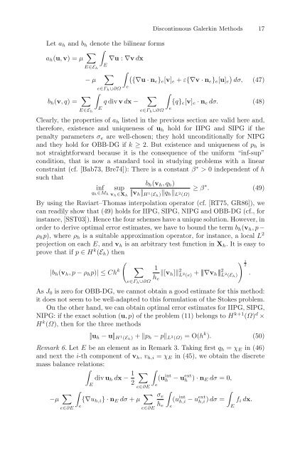
Let a h and b h denote the bilinear forms
a h (u, v) =µ ∑
∇u : ∇v dx
E∈E h
∫E
− µ
b h (v,q)= ∑
E∈E h
∫E
∑
e∈Γ h ∪∂Ω
Discontinuous Galerkin Methods 17
∫
( )
{∇u · ne } e [v] e + ε{∇v · n e } e [u] e dσ, (47)
e
q div v dx −
∑
e∈Γ h ∪∂Ω
∫
{q} e [v] e · n e dσ. (48)
Clearly, the properties of a h listed in the previous section are valid here and,
therefore, existence and uniqueness of u h hold for IIPG and SIPG if the
penalty parameters σ e are well-chosen; they hold unconditionally for NIPG
and they hold for OBB-DG if k ≥ 2. But existence and uniqueness of p h is
not straightforward because it is the consequence of the uniform “inf-sup”
condition, that is now a standard tool in studying problems with a linear
constraint (cf. [Bab73, Bre74]): There is a constant β ∗ > 0 independent of h
such that
b h (v h ,q h )
inf sup
≥ β ∗ . (49)
q h ∈M h v h ∈X h
[|v h |] H 1 (E h )‖q h ‖ L 2 (Ω)
By using the Raviart–Thomas interpolation operator (cf. [RT75, GR86]), we
can readily show that (49) holds for IIPG, SIPG, NIPG and OBB-DG (cf., for
instance, [SST03]). Hence the four schemes have a unique solution. However, in
order to derive optimal error estimates, we have to bound the term b h (v h ,p−
ρ h p), where ρ h is a suitable approximation operator, for instance, a local L 2
projection on each E, andv h is an arbitrary test function in X h .Itiseasyto
prove that if p ∈ H k (E h )then
( ) 1
∑
2
|b h (v h ,p− ρ h p)| ≤Ch k 1
‖[v h ]‖ 2 L
h 2 (e) + |||∇v h||| 2 L 2 (E h ) .
e
e∈Γ h ∪∂Ω
As J 0 is zero for OBB-DG, we cannot obtain a good estimate for this method:
it does not seem to be well-adapted to this formulation of the Stokes problem.
On the other hand, we can obtain optimal error estimates for IIPG, SIPG,
NIPG: if the exact solution (u,p) of the problem (11) belongs to H k+1 (Ω) d ×
H k (Ω), then for the three methods
[|u h − u|] H1 (E h ) + ‖p h − p‖ L2 (Ω) =O(h k ). (50)
Remark 6. Let E be an element as in Remark 3. Taking first q h = χ E in (46)
and next the i-th component of v h , v h,i = χ E in (45), we obtain the discrete
mass balance relations:
∫
div u h dx − 1 ∑
∫
(u int
h − u ext
h ) · n E dσ =0,
E 2 e
e∈∂E
−µ ∑ ∫
{∇u h,i }·n E dσ + µ ∑
e∈∂E
e
e∈∂E
e
σ e
(u
h e
∫e
int
h,i − u ext
h,i ) dσ =
∫
E
f i dx.