Partial Differential Equations - Modelling and ... - ResearchGate

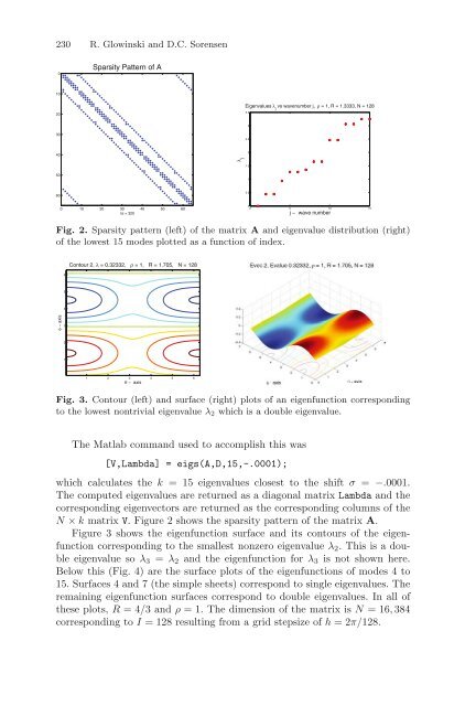
230 R. Glowinski and D.C. Sorensen
0
Sparsity Pattern of A
10
Eigenvalues λ j
vs wavenumber j, ρ = 1, R = 1.3333, N = 128
20
3.5
3
30
2.5
40
2
λ j
1.5
50
1
60
0.5
0 10 20 30 40 50 60
nz = 320
0
0 5 10 15
j − wave number
Fig. 2. Sparsity pattern (left) of the matrix A and eigenvalue distribution (right)
of the lowest 15 modes plotted as a function of index.
Contour 2, λ = 0.32332, ρ = 1, R = 1.705, N = 128
6
5
4
φ − axis
3
2
1
1 2 3 4 5 6
θ − axis
Fig. 3. Contour (left) and surface (right) plots of an eigenfunction corresponding
to the lowest nontrivial eigenvalue λ 2 which is a double eigenvalue.
The Matlab command used to accomplish this was
[V,Lambda] = eigs(A,D,15,-.0001);
which calculates the k = 15 eigenvalues closest to the shift σ = −.0001.
The computed eigenvalues are returned as a diagonal matrix Lambda and the
corresponding eigenvectors are returned as the corresponding columns of the
N × k matrix V. Figure 2 shows the sparsity pattern of the matrix A.
Figure 3 shows the eigenfunction surface and its contours of the eigenfunction
corresponding to the smallest nonzero eigenvalue λ 2 . This is a double
eigenvalue so λ 3 = λ 2 and the eigenfunction for λ 3 is not shown here.
Below this (Fig. 4) are the surface plots of the eigenfunctions of modes 4 to
15. Surfaces 4 and 7 (the simple sheets) correspond to single eigenvalues. The
remaining eigenfunction surfaces correspond to double eigenvalues. In all of
these plots, R =4/3 andρ = 1. The dimension of the matrix is N =16, 384
corresponding to I = 128 resulting from a grid stepsize of h =2π/128.