Partial Differential Equations - Modelling and ... - ResearchGate
Partial Differential Equations - Modelling and ... - ResearchGate
Partial Differential Equations - Modelling and ... - ResearchGate
Create successful ePaper yourself
Turn your PDF publications into a flip-book with our unique Google optimized e-Paper software.
182 B. Maury<br />
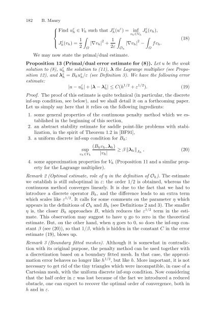
⎧<br />
⎪⎨<br />
Find u ε h ∈ V h such that Jh(u ε ε ) = inf Jh(v ε h ),<br />
v h ∈V h<br />
⎪⎩ Jh(v ε h )= 1 ∫<br />
|∇v h | 2 + 1 ∫<br />
∫<br />
|∇v h | 2 − fv h .<br />
2 Ω 2ε O h Ω<br />
(18)<br />
We may now state the primal/dual estimate.<br />
Proposition 13 (Primal/dual error estimate for (8)). Let u be the weak<br />
solution to (8), u ε h<br />
the solution to (11), λ the Lagrange multiplier (see Proposition<br />
12), <strong>and</strong> λ ε h = B hu ε h<br />
/ε (see Definition 3). We have the following error<br />
estimate:<br />
|u − u ε h| + |λ − λ ε h|≤C(h 1/2 + ε 1/2 ). (19)<br />
Proof. The proof of this estimate is quite technical (in particular, the discrete<br />
inf-sup condition, see below), <strong>and</strong> we shall detail it on a forthcoming paper.<br />
Let us simply say here that it relies on the following ingredients:<br />
1. some general properties of the continuous penalty method which we established<br />
in the beginning of this section,<br />
2. an abstract stability estimate for saddle point-like problems with stabilization,<br />
in the spirit of Theorem 1.2 in [BF91],<br />
3. a uniform discrete inf-sup condition for B h :<br />
(B h v h , λ h )<br />
sup<br />
≥ β ‖λ h ‖<br />
v h ∈V h<br />
|v h |<br />
Λh<br />
, (20)<br />
4. some approximation properties for V h (Proposition 11 <strong>and</strong> a similar property<br />
for the Lagrange multiplier).<br />
Remark 2 (Optimal estimate, role of η in the definition of O h ). The estimate<br />
we establish is still suboptimal in ε: the order 1/2 is obtained, whereas the<br />
continuous method converges linearly. It is due to the fact that we had to<br />
introduce a discrete operator B h , <strong>and</strong> the difference leads to an extra term<br />
which scales like ε 1/2 . It calls for some comments on the parameter η which<br />
appears in the definitions of O h <strong>and</strong> B h (see Definitions 2 <strong>and</strong> 3). The smaller<br />
η is, the closer B h approaches B, which reduces the ε 1/2 term in the estimate.<br />
This observation may suggest to have η go to zero in the theoretical<br />
estimate. But, on the other h<strong>and</strong>, when η goes to 0, so does the inf-sup constant<br />
β (see (20)), so that 1/β, which is hidden in the constant C in the error<br />
estimate (19), blows up.<br />
Remark 3 (Boundary fitted meshes). Although it is somewhat in contradiction<br />
with its original purpose, the penalty method can be used together with<br />
a discretization based on a boundary fitted mesh. In that case, the approximation<br />
error behaves no longer like h 1/2 , but like h. More important, it is not<br />
necessary to get rid of the tiny triangles which were incompatible, in case of a<br />
Cartesian mesh, with the uniform discrete inf-sup condition. Now considering<br />
that the half order in ε was lost because of the fact we introduced a reduced<br />
obstacle, one can expect to recover the optimal order of convergence, both in<br />
h <strong>and</strong> in ε.


