Partial Differential Equations - Modelling and ... - ResearchGate
Partial Differential Equations - Modelling and ... - ResearchGate Partial Differential Equations - Modelling and ... - ResearchGate
The von Neumann Triple Point Paradox 125 2.5 2 1.5 1 0.5 0 −2 −1 0 1 2 Fig. 9. The geometry of the M =1.04/11.5 ◦ Euler example. The insert indicates the region where extreme local grid refinement is performed. to exactly agree with this shock located at x =1.04. The lower boundary condition mimics symmetry about the x-axis for x0. The grid geometry can be seen in Figure 9. This problem is well outside the range where regular reflection solutions are possible. Refer again to the figure to see that its numerical solution (under the insert) clearly resembles single Mach reflection. However, Mach reflection (where three plane shocks meet at a point) is also not possible for a shock this weak [Hen87]. This example demonstrates a classic von Neumann triple point paradox. This problem is solved in self-similar coordinates by essentially the same high order Roe method discussed in the previous section. However, we simplify the Roe approach by again evaluating the Roe matrix at the midpoint, which for the Euler equations is only an approximation to the Roe average. Also, to avoid spurious expansion shocks, artificial dissipation on the order of O(|U r − U l |) is appended to the diagonal part of the Roe dissipation matrix in a field by field manner. We locally refine a very small neighborhood around the apparent triple point as done earlier. The full finest grid has eleven million grid points with 800 × 2000 = 1.6 × 10 6 (∆x ≈ 5 × 10 −7 ) devoted to the local refinement. We plot the sonic number M which is defined as follows. The eigenvalue corresponding to a fast shock in unit direction n for the self-similar Euler flux Jacobian is λ =(u − ξ,v − η) · n + c where ξ = x/t and η = y/t. Define r 2 = ξ 2 + η 2 and set n = (ξ,η)/r, u n =(u, v) · n to find ( un − r λ = c c ) +1 = c(1 −M) where M = r − u n . c
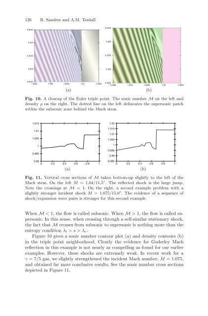
126 R. Sanders and A.M. Tesdall 0.3045 0.3045 0.304 0.304 0.3035 0.3035 0.303 0.303 0.3025 1.0385 1.039 1.0395 1.04 1.0405 (a) 0.3025 1.0385 1.039 1.0395 1.04 1.0405 (b) Fig. 10. A closeup of the Euler triple point. The sonic number M on the left and density ρ on the right. The dotted line on the left delineates the supersonic patch within the subsonic zone behind the Mach stem. 1.015 1.01 1.005 1 0.995 0.99 0 0.2 0.4 0.6 0.8 1 (a) 1.02 1.015 1.01 1.005 1 0.995 0.99 0.985 0 0.2 0.4 0.6 0.8 1 (b) Fig. 11. Vertical cross sections of M taken bottom-up slightly to the left of the Mach stem. On the left M =1.04/11.5 ◦ . The reflected shock is the large jump. Note the crossings at M = 1. On the right, a second example problem with a slightly stronger incident shock M =1.075/15.0 ◦ . The evidence of a sequence of shock/expansion wave pairs is stronger for this second example. When M < 1, the flow is called subsonic. When M > 1, the flow is called supersonic. In this sense, when crossing through a self-similar stationary shock, the fact that M crosses from subsonic to supersonic is nothing more than the entropy condition λ l >s>λ r . Figure 10 gives a sonic number contour plot (a) and density contours (b) in the triple point neighborhood. Clearly the evidence for Guderley Mach reflection in this example is not nearly as compelling as found for our earlier examples. However, these shocks are extremely weak. In recent work for a γ =7/5 gas, we slightly strengthened the incident Mach number, M =1.075, and obtained far more conclusive results. See the sonic number cross sections depicted in Figure 11.
- Page 81 and 82: Optimal Higher Order Time Discretiz
- Page 83 and 84: Optimal Higher Order Time Discretiz
- Page 85 and 86: Optimal Higher Order Time Discretiz
- Page 87 and 88: Optimal Higher Order Time Discretiz
- Page 89 and 90: Optimal Higher Order Time Discretiz
- Page 91 and 92: Optimal Higher Order Time Discretiz
- Page 93 and 94: Optimal Higher Order Time Discretiz
- Page 95 and 96: Optimal Higher Order Time Discretiz
- Page 97 and 98: Optimal Higher Order Time Discretiz
- Page 99 and 100: Optimal Higher Order Time Discretiz
- Page 101 and 102: Optimal Higher Order Time Discretiz
- Page 103 and 104: 96 I. Sazonov et al. To provide a p
- Page 105 and 106: 98 I. Sazonov et al. In the first s
- Page 107 and 108: 100 I. Sazonov et al. Fig. 1. An ex
- Page 109 and 110: 102 I. Sazonov et al. H z 1 exact F
- Page 111 and 112: 104 I. Sazonov et al. (a) (b) Fig.
- Page 113 and 114: 106 I. Sazonov et al. Scattering Wi
- Page 115 and 116: 108 I. Sazonov et al. 6.4 Scatterin
- Page 117 and 118: 110 I. Sazonov et al. (a) (b) Fig.
- Page 119 and 120: 112 I. Sazonov et al. [MHP96] K. Mo
- Page 121 and 122: 114 R. Sanders and A.M. Tesdall I R
- Page 123 and 124: 116 R. Sanders and A.M. Tesdall imp
- Page 125 and 126: 118 R. Sanders and A.M. Tesdall alo
- Page 127 and 128: 120 R. Sanders and A.M. Tesdall (a)
- Page 129 and 130: 122 R. Sanders and A.M. Tesdall D C
- Page 131: 124 R. Sanders and A.M. Tesdall 8.6
- Page 135 and 136: 128 R. Sanders and A.M. Tesdall [TR
- Page 137 and 138: 132 S. Lapin et al. Ω R γ Ω 2 Γ
- Page 139 and 140: 134 S. Lapin et al. ∫ ∂ 2 ∫
- Page 141 and 142: 136 S. Lapin et al. Ω R γ Fig. 3.
- Page 143 and 144: 138 S. Lapin et al. 4 Energy Inequa
- Page 145 and 146: 140 S. Lapin et al. 5 Numerical Exp
- Page 147 and 148: 142 S. Lapin et al. Fig. 6. Contour
- Page 149 and 150: 144 S. Lapin et al. Fig. 9. Obstacl
- Page 151 and 152: Domain Decomposition and Electronic
- Page 153 and 154: Domain Decomposition Approach for C
- Page 155 and 156: Domain Decomposition Approach for C
- Page 157 and 158: Domain Decomposition Approach for C
- Page 159 and 160: Domain Decomposition Approach for C
- Page 161 and 162: Domain Decomposition Approach for C
- Page 163 and 164: Domain Decomposition Approach for C
- Page 165 and 166: Domain Decomposition Approach for C
- Page 167 and 168: Domain Decomposition Approach for C
- Page 169 and 170: Numerical Analysis of a Finite Elem
- Page 171 and 172: Numerical Analysis of a Finite Elem
- Page 173 and 174: Numerical Analysis of a Finite Elem
- Page 175 and 176: Numerical Analysis of a Finite Elem
- Page 177 and 178: Numerical Analysis of a Finite Elem
- Page 179 and 180: Numerical Analysis of a Finite Elem
- Page 181 and 182: so that |u| 2 1,ω h ≤ 2 Numerica
126 R. S<strong>and</strong>ers <strong>and</strong> A.M. Tesdall<br />
0.3045<br />
0.3045<br />
0.304<br />
0.304<br />
0.3035<br />
0.3035<br />
0.303<br />
0.303<br />
0.3025<br />
1.0385 1.039 1.0395 1.04<br />
1.0405<br />
(a)<br />
0.3025<br />
1.0385 1.039 1.0395 1.04<br />
1.0405<br />
(b)<br />
Fig. 10. A closeup of the Euler triple point. The sonic number M on the left <strong>and</strong><br />
density ρ on the right. The dotted line on the left delineates the supersonic patch<br />
within the subsonic zone behind the Mach stem.<br />
1.015<br />
1.01<br />
1.005<br />
1<br />
0.995<br />
0.99<br />
0 0.2 0.4 0.6 0.8 1<br />
(a)<br />
1.02<br />
1.015<br />
1.01<br />
1.005<br />
1<br />
0.995<br />
0.99<br />
0.985<br />
0 0.2 0.4 0.6 0.8 1<br />
(b)<br />
Fig. 11. Vertical cross sections of M taken bottom-up slightly to the left of the<br />
Mach stem. On the left M =1.04/11.5 ◦ . The reflected shock is the large jump.<br />
Note the crossings at M = 1. On the right, a second example problem with a<br />
slightly stronger incident shock M =1.075/15.0 ◦ . The evidence of a sequence of<br />
shock/expansion wave pairs is stronger for this second example.<br />
When M < 1, the flow is called subsonic. When M > 1, the flow is called supersonic.<br />
In this sense, when crossing through a self-similar stationary shock,<br />
the fact that M crosses from subsonic to supersonic is nothing more than the<br />
entropy condition λ l >s>λ r .<br />
Figure 10 gives a sonic number contour plot (a) <strong>and</strong> density contours (b)<br />
in the triple point neighborhood. Clearly the evidence for Guderley Mach<br />
reflection in this example is not nearly as compelling as found for our earlier<br />
examples. However, these shocks are extremely weak. In recent work for a<br />
γ =7/5 gas, we slightly strengthened the incident Mach number, M =1.075,<br />
<strong>and</strong> obtained far more conclusive results. See the sonic number cross sections<br />
depicted in Figure 11.


