Partial Differential Equations - Modelling and ... - ResearchGate

More documents

Recommendations

Info

Electromagnetic Scattering 99 purpose, we choose to employ the Delaunay–Voronoï dual diagram, with the integrals taken over the edges of the Delaunay and Voronoï cells. To illustrate the process, consider a triangular element m of the Delaunay mesh. This element will share an edge with N m elements, with numbers m i ,1≤ i ≤ N m , where N m = 3, unless the element has an edge representing the boundary of the domain. Suppose the Delaunay edge mm i is the common edge between elements m and m i and let the length of this edge be denoted by l mmi . Similarly, suppose that the Voronoï edgemm i is the line segment connecting the circumcentres of element m and element m i . The length of this Voronoï edge will be denoted by h mmi . As basic unknowns in the solution algorithm, we consider the value of the z-component of the magnetic field at the Voronoï vertices, and denote this by H m , and the projection of the electric field at the midpoint of the Delaunay edge mm i , in the direction of the edge, and denote this by E mmi . In this case, the laws of Ampère and Faraday can be approximated, using central differencing, as H (n+1/2) m E (n+1) mm i = H (n−1/2) m − ∆t ∑N m S m i=1 E (n) mm i l mmi , (11) = E mm (n) i + ∆t [ ] H m (n+1/2) − H m (n+1/2) h i , (12) mmi where S m is the area of element m. This is a staggered explicit scheme, where the time step size for a stable implementation may be determined from the requirement [TH00] ∆t < C min {l min ,h min } . (13) Here l min and h min are the minimum Delaunay and Voronoï edge lengths respectively and C is a safety factor. This implies the use of meshes which do not include either very short Delaunay, or very short Voronoï, edges. However, Voronoï edge lengths may vanish completely, on a general unstructured mesh, when two adjacent triangles have a common circumcentre. When this happens, the simple remedy is to merge these two triangles to form a single quadrilateral element. The discrete formulae of the equations (11) and (12) may be applied directly to this quadrilateral, with appropriate redefinition of N m . Moreover, the same merging procedure can be adopted when more than two triangles share a common circumcentre and the discrete equations applied again to the polygonal cell that is created by merging the triangles in this manner. This merging process is illustrated in Figure 1. If the mesh contains short non-zero Voronoï sides, the merging process may still be carried out, to overcome the severe restriction on the time step. However, this will reduce the accuracy of the scheme, due to the slight local non-orthogonality introduced by the merging. The boundary condition on the tangential component of the electric field can be directly imposed at the surface of the PEC. The far field boundary condition is again approximated by the addition of an artificial PML, with the external boundary of the truncated domain taken to be rectangular in shape.
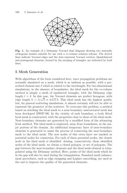
100 I. Sazonov et al. Fig. 1. An example of a Delaunay–Voronoï dual diagram showing two mutually orthogonal meshes suitable for use with a co-volume solution scheme. The dotted lines indicate Voronoï edges and the dots represent Voronoï vertices. Quadrilateral and pentagonal elements, formed by the merging of triangles, are indicated by bold lines. 5 Mesh Generation With algorithms of the form considered here, wave propagation problems are normally simulated on a mesh, which is as uniform as possible, with a prescribed element size δ which is related to the wavelength. For two-dimensional simulations, in the absence of boundaries, the ideal mesh for the co-volume method is simply a mesh of equilateral triangles, with the Delaunay edge length l = δ. In this case, the Voronoï elements are perfect hexagons, with edge length h = δ/ √ 3 ≈ 0.577 δ. This ideal mesh has the highest quality but, for general scattering simulations, it almost certainly will not be able to represent the geometry of the scatterer. To overcome this problem, a method based on stitching the ideal mesh to a near-boundary unstructured mesh has been developed [SWH + 06]. In the vicinity of each boundary, a body fitted local mesh is constructed, with the properties close to those of the ideal mesh. Near-boundary elements are generated by a modified form of the advancing front method. The ideal mesh is employed, away from boundaries, in the major portion of the domain. An additional temporary layer of near-boundary elements is generated to assist the process of connecting the near-boundary mesh to the ideal mesh. The new nodes of this extra layer are marked as potential nodes for connection. For each of these potential nodes, the closest node in the ideal mesh is identified. Joining, consecutively, these identified nodes of the ideal mesh, we obtain a closed polygon, or set of polygons. The gap between the near-boundary elements and the ideal mesh element is triangulated using the Delaunay method. Here, points of the ideal mesh which lie in the gap will also be used during the triangulation. Standard mesh enhancement procedures, such as edge swapping and Laplace smoothing, are used at the end to improve the quality of the generated elements.
Page 1 and 2:
Partial Differential Equations
Page 3 and 4:
Partial Differential Equations Mode
Page 5 and 6:
Dedicated to Olivier Pironneau
Page 7 and 8:
VIII Preface computers has been at
Page 9 and 10:
Contents List of Contributors .....
Page 11 and 12:
List of Contributors Yves Achdou UF
Page 13 and 14:
List of Contributors XV Claude Le B
Page 15 and 16:
Discontinuous Galerkin Methods Vive
Page 17 and 18:
Discontinuous Galerkin Methods 5 2
Page 19 and 20:
Discontinuous Galerkin Methods 7 g
Page 21 and 22:
Discontinuous Galerkin Methods 9 (
Page 23 and 24:
Page 25 and 26:
Page 27 and 28:
Discontinuous Galerkin Methods 15 W
Page 29 and 30:
Let a h and b h denote the bilinear
Page 31 and 32:
Discontinuous Galerkin Methods 19 t
Page 33 and 34:
Discontinuous Galerkin Methods 21 l
Page 35 and 36:
Table 1. Primal DG for transport Di
Page 37 and 38:
Discontinuous Galerkin Methods 25 [
Page 39 and 40:
Mixed Finite Element Methods on Pol
Page 41 and 42:
Mixed FE Methods on Polyhedral Mesh
Page 43 and 44:
Page 45 and 46:
Page 47 and 48:
4 Hybridization and Condensation Mi
Page 49 and 50:
Page 51 and 52:
is symmetric and positive definite,
Page 53 and 54:
with some coefficient α ∈ R wher
Page 55 and 56: 44 E.J. Dean and R. Glowinski so fa
Page 57 and 58: 46 E.J. Dean and R. Glowinski 2 A L
Page 59 and 60: 48 E.J. Dean and R. Glowinski S:T=
Page 61 and 62: 50 E.J. Dean and R. Glowinski minim
Page 63 and 64: 52 E.J. Dean and R. Glowinski 6 On
Page 65 and 66: 54 E.J. Dean and R. Glowinski Fig.
Page 67 and 68: 56 E.J. Dean and R. Glowinski and
Page 69 and 70: 58 E.J. Dean and R. Glowinski 7 Num
Page 71 and 72: 60 E.J. Dean and R. Glowinski Fig.
Page 73 and 74: 62 E.J. Dean and R. Glowinski Assum
Page 75 and 76: Higher Order Time Stepping for Seco
Page 77 and 78: u n+1 h Optimal Higher Order Time D
Page 79 and 80: Optimal Higher Order Time Discretiz
Page 103 and 104: 96 I. Sazonov et al. To provide a p
Page 105: 98 I. Sazonov et al. In the first s
Page 109 and 110: 102 I. Sazonov et al. H z 1 exact F
Page 111 and 112: 104 I. Sazonov et al. (a) (b) Fig.
Page 113 and 114: 106 I. Sazonov et al. Scattering Wi
Page 115 and 116: 108 I. Sazonov et al. 6.4 Scatterin
Page 117 and 118: 110 I. Sazonov et al. (a) (b) Fig.
Page 119 and 120: 112 I. Sazonov et al. [MHP96] K. Mo
Page 121 and 122: 114 R. Sanders and A.M. Tesdall I R
Page 123 and 124: 116 R. Sanders and A.M. Tesdall imp
Page 125 and 126: 118 R. Sanders and A.M. Tesdall alo
Page 127 and 128: 120 R. Sanders and A.M. Tesdall (a)
Page 129 and 130: 122 R. Sanders and A.M. Tesdall D C
Page 131 and 132: 124 R. Sanders and A.M. Tesdall 8.6
Page 133 and 134: 126 R. Sanders and A.M. Tesdall 0.3
Page 135 and 136: 128 R. Sanders and A.M. Tesdall [TR
Page 137 and 138: 132 S. Lapin et al. Ω R γ Ω 2 Γ
Page 139 and 140: 134 S. Lapin et al. ∫ ∂ 2 ∫
Page 141 and 142: 136 S. Lapin et al. Ω R γ Fig. 3.
Page 143 and 144: 138 S. Lapin et al. 4 Energy Inequa
Page 145 and 146: 140 S. Lapin et al. 5 Numerical Exp
Page 147 and 148: 142 S. Lapin et al. Fig. 6. Contour
Page 149 and 150: 144 S. Lapin et al. Fig. 9. Obstacl
Page 151 and 152: Domain Decomposition and Electronic
Page 153 and 154: Domain Decomposition Approach for C
Page 155 and 156: Domain Decomposition Approach for C
Page 157 and 158:
Domain Decomposition Approach for C
Page 159 and 160:
Page 161 and 162:
Page 163 and 164:
Page 165 and 166:
Page 167 and 168:
Page 169 and 170:
Numerical Analysis of a Finite Elem
Page 171 and 172:
Page 173 and 174:
Page 175 and 176:
Page 177 and 178:
Page 179 and 180:
Page 181 and 182:
so that |u| 2 1,ω h ≤ 2 Numerica
Page 183 and 184:
Page 185 and 186:
Page 187 and 188:
Page 189 and 190:
188 A. Bonito et al. of the model a
Page 191 and 192:
190 A. Bonito et al. Fig. 1. The sp
Page 193 and 194:
192 A. Bonito et al. 3 1 16 4 1 1 1
Page 195 and 196:
194 A. Bonito et al. ∫ v n+1 h
Page 197 and 198:
196 A. Bonito et al. −pn +2µD(v)
Page 199 and 200:
198 A. Bonito et al. each of its pa
Page 201 and 202:
200 A. Bonito et al. The normal vec
Page 203 and 204:
202 A. Bonito et al. with initial c
Page 205 and 206:
204 A. Bonito et al. Fig. 8. Jet bu
Page 207 and 208:
206 A. Bonito et al. References [AM
Page 209 and 210:
208 A. Bonito et al. [Set96] J. A.
Page 211 and 212:
210 J. Hao et al. due to shear flow
Page 213 and 214:
212 J. Hao et al. The backward reac
Page 215 and 216:
214 J. Hao et al. where u and p den
Page 217 and 218:
216 J. Hao et al. * * * * * * * * *
Page 219 and 220:
218 J. Hao et al. and solve for V n
Page 221 and 222:
220 J. Hao et al. Table 2. The calc
Page 223 and 224:
222 J. Hao et al. References [ASS80
Page 225 and 226:
Computing the Eigenvalues of the La
Page 227 and 228:
Eigenvalues of the Laplace-Beltrami
Page 229 and 230:
Page 231 and 232:
Page 233 and 234:
A Fixed Domain Approach in Shape Op
Page 235 and 236:
Shape Optimization Problems with Ne
Page 237 and 238:
Page 239 and 240:
Page 241 and 242:
Page 243 and 244:
Reduced-Order Modelling of Dispersi
Page 245 and 246:
Page 247 and 248:
Page 249 and 250:
Page 251 and 252:
Page 253 and 254:
Page 255 and 256:
Calibration of Lévy Processes with
Page 257 and 258:
Page 259 and 260:
Page 261 and 262:
Page 263 and 264:
We have proved Calibration of Lévy
Page 265 and 266:
Page 267 and 268:
Page 269 and 270:
Page 271 and 272:
Note that p ∗ satisfies Calibrati
Page 273 and 274:
Page 275 and 276:
280 S. Ikonen and J. Toivanen the p
Page 277 and 278:
282 S. Ikonen and J. Toivanen Merto
Page 279 and 280:
284 S. Ikonen and J. Toivanen For H
Page 281 and 282:
286 S. Ikonen and J. Toivanen and {
Page 283 and 284:
288 S. Ikonen and J. Toivanen 1.6 1
Page 285 and 286:
290 S. Ikonen and J. Toivanen 8 Con
Page 287:
292 S. Ikonen and J. Toivanen [Mer7
show all

Partial Differential Equations - Modelling and ... - ResearchGate

Create successful ePaper yourself

Delete template?

Save as template?