Biodiversity Data Analysis: Testing Statistical Hypotheses
Biodiversity Data Analysis: Testing Statistical Hypotheses
Biodiversity Data Analysis: Testing Statistical Hypotheses

Create successful ePaper yourself
Turn your PDF publications into a flip-book with our unique Google optimized e-Paper software.
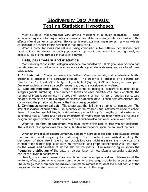
<strong>Biodiversity</strong> <strong>Data</strong> <strong>Analysis</strong>:<br />
<strong>Testing</strong> <strong>Statistical</strong> <strong>Hypotheses</strong><br />
Most biological measurements vary among members of a study population. These<br />
variations may occur for any number of reasons, from differences in genetic expression to the<br />
effects of environmental variables. Hence, an investigator must measure as many individuals<br />
as possible to account for the variation in that population.<br />
When a particular measured value is being compared in two different populations, care<br />
must be taken to ensure that each population is represented as accurately and rigorously as<br />
possible. This is the purpose of statistical analysis.<br />
I. <strong>Data</strong>, parameters and statistics<br />
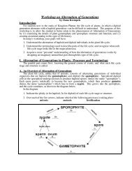
Many investigations in the biological sciences are quantitative. Biological observations can<br />
be tabulated as numerical facts, also known as data (singular = datum), and can be of three<br />
basic types.<br />
1. Attribute data. These are descriptive, "either-or" measurements, and usually describe the<br />
presence or absence of a particular attribute. The presence or absence of a genetic trait<br />
("freckles" or "no freckles") or the type of genetic trait (type A, B, AB or o blood) are examples.<br />
Because such data have no specific sequence, they are considered unordered.<br />
2. Discrete numerical data. These correspond to biological observations counted as<br />
integers (whole numbers). The number of leaves on each member of a group of plants, the<br />
number of breaths per minute in a group of newborns or the number of beetles per square<br />
meter of forest floor are all examples of discrete numerical data. These data are ordered, but<br />
do not describe physical attributes of the things being counted.<br />
3. Continuous numerical data. These are data that fall along a numerical continuum. The<br />
limit of resolution of such data is the accuracy of the methods and instruments used to collect<br />
them. Examples are tail length, brain volume, percent body fat...anything that varies on a<br />
continuous scale. Rates (such as decomposition of hydrogen peroxide per minute or uptake of<br />
oxygen during respiration over the course of an hour) are also numerical continuous data.<br />
When you perform an experiment, you must know which type of data you are collecting.<br />
The statistical test appropriate for a particular data set depends upon the nature of the data.<br />
When an investigator collects numerical data from a group of subjects, s/he must determine<br />
how and with what frequency the data vary. For example, if one wished to study the<br />
distribution of shoe size in the human population, one might measure the shoe size of a<br />
sample of the human population (say, 50 individuals) and graph the numbers with "shoe size"<br />
on the x-axis and "number of individuals" on the y-axis. The resulting figure shows the<br />
frequency distribution of the data, a representation of how often a particular data point<br />
occurs at a given measurement.<br />
Usually, data measurements are distributed over a range of values. Measures of the<br />
tendency of measurements to occur near the center of the range include the population mean<br />
(the average measurement), the median (the measurement located at the exact center of the<br />
range) and the mode (the most common measurement in the range).<br />
<strong>Biodiversity</strong> – <strong>Data</strong> <strong>Analysis</strong> 1
It is also important to understand how much variation a group of subjects exhibits around<br />
the mean. For example, if the average human shoe size is "9," we must determine whether<br />
shoe size forms a very wide distribution (with a relatively small number of individuals wearing<br />
all sizes from 1 - 15) or one which hovers near the mean (with a relatively large number of<br />
individuals wearing sizes 7 through 10, and many fewer wearing sizes 1-6 and 11-15).<br />
Measurements of dispersion around the mean include the range, variance and standard<br />
deviation.<br />
Parameters and Statistics<br />
If you were able to measure the height of every adult male Homo sapiens who ever existed,<br />
and then calculate a mean, median, mode, range, variance and standard deviation from your<br />
measurements, those values would be known as parameters. They represent the actual<br />
values as calculated from measuring every member of a population of interest. Obviously, it is<br />
very difficult to obtain data from every member of a population of interest, and impossible of<br />
that population is theoretically infinite in size. However, one can estimate parameters by<br />
randomly sampling members of the population. Such an estimate, calculated from<br />
measurements of a subset of the entire population, is known as a statistic.<br />
In general, parameters are written as Greek symbols equivalent to the Roman symbols<br />
used to represent statistics. For example, the standard deviation for a subset of an entire<br />
population is written as "s", whereas the true population parameter is written as σ.<br />
Statistics and statistical tests are used to test whether the results of an experiment are<br />
significantly different from what is expected. What is meant by "significant?" For that matter,<br />
what is meant by "expected" results? To answer these questions, we must consider the<br />
matter of probability.<br />
II. Experimental Design for <strong>Statistical</strong> <strong>Hypotheses</strong><br />
As you know from reading Appendix I, statistical hypotheses are stated in terms of two<br />
opposing statements, the null hypothesis (H o ) and the alternative hypothesis (H a ). The null<br />
hypothesis states that there is no significant difference between two populations being<br />
compared. The alternative hypothesis may be either directional (one-tailed), stating the<br />
precise way in which the two populations will differ, or nondirectional (two-tailed), not<br />
specifying the way in which two populations will differ.<br />
For example, if you were testing the efficacy of a new drug (Fat-B-Gon ) in promoting<br />
tm)<br />
weight loss in a population of volunteer subjects, you would assemble two groups of volunteers<br />
who are as similar as possible in every aspect (age, sex, weight, health measurements, etc.),<br />
and divide them into two groups. One half of the subjects (the treatment group) would receive<br />
the drug, and the other half (the control group) would receive an inert substance, known as a<br />
placebo, that subjects cannot distinguish from the actual drug. Both groups would be<br />
administered either the drug or the placebo in exactly the same way. Subjects must not know<br />
whether they are in the treatment or control group (a single-blind study), as this will help to<br />
prevent the placebo effect, a measurable, observable change in health or behavior not<br />
attributable to a medication or other treatment. The placebo effect is believed to be triggered<br />
by a subject’s belief that a medication or treatment will have a certain result. In some cases,<br />
not even the investigators know which subjects are in the treatment and control groups (a<br />
double-blind study). Thus, the only difference between the treatment and control groups<br />
<strong>Biodiversity</strong> – <strong>Data</strong> <strong>Analysis</strong> 2
is the presence or absence of a single variable, in this case, Fat-B-Gon tm . Such careful<br />
design and execution of the experiment reduces the influence of confounding effects,<br />
uncontrolled differences between the two groups that might affect the results.<br />
Over the course of the experiment, our investigators measure weight changes in each<br />
individual of both groups (Table 1). Because they cannot control for the obvious confounding<br />
effect of genetic differences in metabolism, the investigators must try to reduce the influence of<br />
that effect by using a large sample size--as many experimental subjects as possible--so there<br />
will be a wide variety of metabolic types in both the treatment and control groups. The larger<br />
the sample size, the more closely the statistic will reflect the actual parameter.<br />
Table 1. Change in weight (x) of subjects given Fat-B-Gon tm (treatment) and placebo<br />
(control) food supplements over the course of one month. All weight changes were<br />
negative (weight loss). Mean weight change (x), the square of each data point (x 2 ) and<br />
the squared deviation from the mean (x - x) 2 are included for later statistical analysis.<br />
control Dweight (Dweight) 2 (x - x) 2 treatment Dweight (D weight) 2 (x - x) 2<br />
subjects (kg) (= x) (= x 2 )<br />
subjects (kg) (= x) (= x 2 )<br />
1 4.4 19.36 0.12 11 11.0 121.00 13.40<br />
2 6.3 36.69 2.43 12 5.5 30.25 3.39<br />
3 1.2 1.44 12.53 13 6.2 38.44 1.30<br />
4 7.4 54.76 7.07 14 9.1 82.81 3.10<br />
5 6.0 36.00 1.59 15 8.1 65.61 0.58<br />
6 4.1 16.81 0.41 16 6.0 36.00 1.80<br />
7 5.2 27.04 0.21 17 8.2 67.24 0.74<br />
8 3.1 9.61 2.69 18 5.0 25.00 5.47<br />
9 4.2 17.64 0.29 19 7.2 51.84 0.02<br />
10 5.5 30.25 0.58 20 7.1 50.41 0.06<br />
total (S) 47.4<br />
(x=4.74)<br />
249.6<br />
(=Sx 2 )<br />
III. <strong>Statistical</strong> tests<br />
27.92<br />
(=S(x-x) 2 )<br />
total (S) 73.4<br />
(x = 7.34)<br />
568.60<br />
(=Sx 2 )<br />
29.86<br />
(=S(x-x) 2 )<br />
Let's continue with our Fat-B-Gon tm subjects. After the data have been collected, the<br />
subjects can go home and eat Twinkies T.M. and the investigators' analysis begins. They must<br />
now determine whether any difference in weight loss between the two groups is significant or<br />
simply due to random chance. To do so, the investigators must perform a statistical test on<br />
the data collected. The results of this test will enable them to either ACCEPT or REJECT the<br />
null hypothesis.<br />
A. Mean, variance and standard deviation<br />
You probably will be dealing most often with numerical continuous data, and so should be<br />
familiar with the definitions and abbreviations of several important quantities:<br />
x = data point the individual values of a measured parameter (=x i )<br />
_<br />
x = mean<br />
the average value of a measured parameter<br />
n = sample size<br />
the number of individuals in a particular test group<br />
<strong>Biodiversity</strong> – <strong>Data</strong> <strong>Analysis</strong> 3
df = degrees of freedom<br />
s 2 = variance<br />
the number of independent quantities in a system<br />
a measure of individual data points' variability from the mean<br />
s = standard deviation the positive square root of the variance<br />
To calculate the mean weight change of either the treatment or control group, the<br />
investigators simply sum the weight change of all individuals in a particular group and divide it<br />
by the sample size.<br />
n<br />
_<br />
Σ x i<br />
x = i=1<br />
n<br />
Thus calculated, the mean weight change of our Fat-B-Gon tm control group is 4.74 kg, and of<br />
the treatment group, 7.34 kg (Table A2-1).<br />
To determine the degree of the subjects' variability from the mean weight change, the<br />
investigators calculate several quantities. The first is the sum of squares (SS) of the<br />
deviations from the mean, defined as:<br />
_<br />
SS = Σ ( x - x i ) 2<br />
Whenever there is more than one test group, statistics referring to each test group are given a<br />
subscript as a label. In our example, we will designate any statistic from the control group with<br />
a subscript "c" and any statistic from the treatment group with a subscript "t." Thus, sum of<br />
squares of our control group (SS c ) is equal to 27.92 and SS t is equal to 29.86 (Table A2-2).<br />
The variance (s 2 ) of the data, the mean SS of each test group, is defined as:<br />
Calculate the variance for both the treatment and control Fat-B-Gon tm groups. Check your<br />
answers against the correct ones listed Table A2-2.<br />
Standard deviation (s), the square root of the variance:<br />
Calculate the standard deviation for the treatment and control groups. Check your answers<br />
against the correct ones listed in Table A2-2.<br />
B. Parametric tests<br />
A parametric test is used to test the significance of continuous numerical data (e.g. -<br />
lizard tail length, change in weight, reaction rate, etc.). Examples of commonly used<br />
parametric tests are the Student's t-test and the ANOVA. Your biodiversity data are likely to be<br />
non-parametric, but if you do have parametric data, you should already be familiar with the use<br />
<strong>Biodiversity</strong> – <strong>Data</strong> <strong>Analysis</strong> 4
of the student’s t-test, which will allow you to compare two means (either independent or<br />
paired). If you are not familiar with the t-test, you can find an exercise here:<br />
http://www.bio.miami.edu/dana/151/gofigure/151F11_statistics.pdf<br />
C. Non-parametric tests<br />
A non-parametric test is used to test the significance of qualitative data (e.g. numbers of<br />
purple versus yellow corn kernels, presence or absence of freckles in members of a population<br />
etc.). Both attribute data and discrete numerical data can be analyzed with non-parametric<br />
tests such as the Chi-square and Mann-Whitney U test.<br />
Most of the biodiversity research teams likely collected non-parametric data. If you are<br />
comparing two non-parametric data sets, a useful test, analogous to the parametric t-test, is<br />
the Mann-Whitney U test. A clear explanation of how to use this test can be found on our old<br />
pal YouTube, right here:<br />
Mann-Whitney U: http://www.youtube.com/watch?v=nRAAAp1Bgnw<br />
If your team is comparing more than two non-parametric data sets, a useful test, analogous to<br />
the ANOVA (<strong>Analysis</strong> Of Variance), is the Kruskal-Wallis test. This is nicely explained here:<br />
Kruskal Wallis: http://www.youtube.com/watch?v=BkyGuNuaZYw<br />
IV. Probability and significance<br />
The term "significant" is often used in every day conversation, yet few people know the<br />
statistical meaning of the word. In scientific endeavors, significance has a highly specific and<br />
important definition. Every time you read the word "significant" in this book, know that we refer<br />
to the following scientifically accepted standard:<br />
The difference between an observed and expected result is said to be statistically<br />
significant if and only if:<br />
Under the assumption that there is no true difference, the probability that<br />
the observed difference would be at least as large as that actually seen is<br />
less than or equal to 5% (0.05).<br />
Conversely, under the assumption that there is no true difference, the<br />
probability that the observed difference would be smaller than that actually<br />
seen is greater than 95% (0.95).<br />
Once an investigator has calculated a Chi-square or t-statistic, s/he must be able to draw<br />
conclusions from it. How does one determine whether deviations from the expected (null<br />
hypothesis) are significant?<br />
As mentioned previously, depending upon the degrees of freedom, there is a specific<br />
probability value linked to every possible value of any statistic.<br />
<strong>Biodiversity</strong> – <strong>Data</strong> <strong>Analysis</strong> 5
A. Determining the significance level of a parametric statistic<br />
If were to perform an independent sample t- test on the Fat-B-Gon data listed previously,<br />
we might obtain values equal to those listed in Table 2, with a t-statistic equal to 4.05. The<br />
next step is to interpret what this statistic tells us about the difference in mean weight loss<br />
between the treatment and control groups. Is the difference significant, suggesting that Fat-B-<br />
Gon tm is that mysterious factor "other than chance?" Or is the melting of unsightly cellulite at<br />
the pop of a pill just another poor biologist's fantasy of early retirement? The answer lies in the<br />
table of critical values for the t-statistic, part of which is illustrated in Table 3.<br />
Table 2. Treatment and control group statistics and overall statistics for weight<br />
loss in the Fat-B-Gon experiment.<br />
statistic control treatment<br />
mean (x) 4.74 7.34<br />
sum of squares (SS) 27.9 29.9<br />
variance (s2) 2.79 2.99<br />
standard deviation (s) 1.66 1.82<br />
overall statistics<br />
s 2 p<br />
3.21<br />
sxt - s xc<br />
0.642<br />
t 4.05<br />
degrees of freedom (df) 19<br />
P value (significance)<br />
P ><br />
The Fat-B-Gon tm t statistic (4.05) is larger than the greatest value for (df = 19) on the table<br />
of critical values. Thus, the probability that the weight difference in treatment and control<br />
groups is due to chance is less than 0.001 for our two-tailed hypothesis. This is highly<br />
significant. It means that the likelihood that the weight loss difference between the treatment<br />
and control is due to Fat-B-Gon (and not just random chance) is greater than 99%. We thus<br />
can reject our original two-tailed hypothesis and accept the alternative hypothesis:<br />
"There is a difference in the rate of weight loss between members of the<br />
population who use Fat-B-Gon tm and those who do not use Fat-B-Gon tm ."<br />
Notice that the t-value calculated for the Fat-B-Gon tm data indicates rejection of even onetailed<br />
hypothesis. However, because all honest researchers state their hypotheses before<br />
<strong>Biodiversity</strong> – <strong>Data</strong> <strong>Analysis</strong> 6
they see their results, Team Fat-B-Gon tm should stick by their original hypothesis and let the<br />
direction of the data (i.e., all volunteers lost weight) speak for itself.<br />
Remember that you must have a representative sample of the population--not a single<br />
experimental run--in order to perform the t-test (A single experiment cannot have a mean,<br />
variance or standard deviation.). Your probability value will come closer to the population<br />
parameter if your sample size is large.<br />
Table 3. Partial table of critical values for the two-sample t-test. The second row of P values should be<br />
used for a two-tailed alternate hypothesis (i.e., one which does not specify the direction (weight loss or<br />
gain) of the alternate hypothesis). The first row of P values should be used for a one-tailed hypothesis<br />
(i.e., one which does specify the direction of the alternate hypothesis). A t-statistic to the right of the<br />
double bar indicates rejection of the two-tailed Fat-B-Gon tm null hypothesis (at df = 9).<br />
http://www.stattools.net/tTest_Tab.php)<br />
P 0.05 0.025 0.01 0.005 0.0025 0.001 0.0005<br />
(1 tail)<br />
P 0.1 0.05 0.02 0.01 0.005 0.002 0.001<br />
(2 tail)<br />
df<br />
1 6.3138 12.7065 31.8193 63.6551 127.3447 318.4930 636.0450<br />
2 2.9200 4.3026 6.9646 9.9247 14.0887 22.3276 31.5989<br />
3 2.3534 3.1824 4.5407 5.8408 7.4534 10.2145 12.9242<br />
4 2.1319 2.7764 3.7470 4.6041 5.5976 7.1732 8.6103<br />
5 2.0150 2.5706 3.3650 4.0322 4.7734 5.8934 6.8688<br />
6 1.9432 2.4469 3.1426 3.7074 4.3168 5.2076 5.9589<br />
7 1.8946 2.3646 2.9980 3.4995 4.0294 4.7852 5.4079<br />
8 1.8595 2.3060 2.8965 3.3554 3.8325 4.5008 5.0414<br />
9 1.8331 2.2621 2.8214 3.2498 3.6896 4.2969 4.7809<br />
10 1.8124 2.2282 2.7638 3.1693 3.5814 4.1437 4.5869<br />
11 1.7959 2.2010 2.7181 3.1058 3.4966 4.0247 4.4369<br />
12 1.7823 2.1788 2.6810 3.0545 3.4284 3.9296 4.3178<br />
13 1.7709 2.1604 2.6503 3.0123 3.3725 3.8520 4.2208<br />
14 1.7613 2.1448 2.6245 2.9768 3.3257 3.7874 4.1404<br />
15 1.7530 2.1314 2.6025 2.9467 3.2860 3.7328 4.0728<br />
16 1.7459 2.1199 2.5835 2.9208 3.2520 3.6861 4.0150<br />
17 1.7396 2.1098 2.5669 2.8983 3.2224 3.6458 3.9651<br />
18 1.7341 2.1009 2.5524 2.8784 3.1966 3.6105 3.9216<br />
19 1.7291 2.0930 2.5395 2.8609 3.1737 3.5794 3.8834<br />
20 1.7247 2.0860 2.5280 2.8454 3.1534 3.5518 3.8495<br />
(After<br />
B. Determining significance level of a non-parametric statistic<br />
Critical values associated with non-parametric statistics have been compiled for the Mann-<br />
Whitney U appear in Table 4 (Mann-Whitney U). Kruskal Wallis critical values are more<br />
complex, as they involve more than two data sets. Fortunately for us, J. Patrick Meyer<br />
(University of Virginia) and Michael A. Seaman (University of South Caroina) have made<br />
available a limited portion of a table of critical values they have calculated. These can be<br />
found here if your project involves either three or four data sets:<br />
http://faculty.virginia.edu/kruskal-wallis/<br />
<strong>Biodiversity</strong> – <strong>Data</strong> <strong>Analysis</strong> 7
The tables are not complete, but they do provide cricital values for Probability (P) values of 0.1,<br />
0.5, and 0.01. You are unlikely to need other values, as these will tell you whether to accept or<br />
reject your null hypothesis.<br />
Table 4. Critical values for the Mann-Whitney U test. The vertical grey column (n1)<br />
represents the number of samples in your first data set, while the horizontal grey row<br />
(n2) represents the number of samples in your second data set. There are no degrees<br />
of freedom in this table of critical values.<br />
<strong>Biodiversity</strong> – <strong>Data</strong> <strong>Analysis</strong> 8