FAST 3D SCANNING METHODS FOR LASER MEASUREMENT ...

FAST 3D SCANNING METHODS FOR LASER MEASUREMENT SYSTEMS
Oliver Wulf, Bernardo Wagner
Institute for Systems Engineering, University of Hannover, Germany
Email: {wulf,wagner}@rts.uni-hannover.de
Abstract: 3D perception is a promising technology for automatic control, manufacturing
and robotics. Compared to 2D vision systems 3D range sensors can provide direct geometric
information of the environment. This paper describes 3D scanning systems with
laser time-of-flight measurement devices and compares their usability in different application
scenes. Additionally new methods that allow fast scanning are contributed. Optimizations
are based on efficient scanning methods with a maximum number of measurement
points in the area of interest, compensation of systematic measurement errors
and improvements of the mechanical scanning system. All described methods are implemented
and tested on a mobile robot with a real-time Linux system.
Keywords: Data Acquisition Systems, 3D Perception, Laser Range Finder, LMS
1. INTRODUCTION
There are a number of ways to acquire 3-
Dimensional information of the environment. Measuring
methods can be divided into three major principles,
stereo vision (e.g. with application in robotics,
Lacroix et al., 2002), active triangulation (e.g. in
quality control, Perceptron, 2003) and laser time-offlight
measurement (see below). Each method has its
advantages and drawbacks and is therefore suitable
for different applications.
The laser time-of-flight method, that will be dealt
with in this paper, is robust and can provide distance
measurements in a range of more than 50m with
centimeter accuracy. As the measurement device is
1-Dimensional a scanning mirror is needed to get 2D
or 3D data. Commercial 2D sensors that work on this
principle are available and widely used. On the other
hand there is no commercial 3D scanner available
that is suitable for applications in dynamic environments.
Laser scanners that are used in surveying (for
example Riegl, 2001) do not fulfill the needs of factory
automation and robotics, as they are heavy,
expensive and the scan time is by far too long (a few
minutes).
A common solution to make 3D scanning feasible for
this kind of applications is to use a standard 2D scanner
and a mechanical actuator to reach the 3 rd dimension.
The actuator can be a servo drive to turn the
scanner (Surmann et al., 2001 and Hähnel and Burgard,
2002).
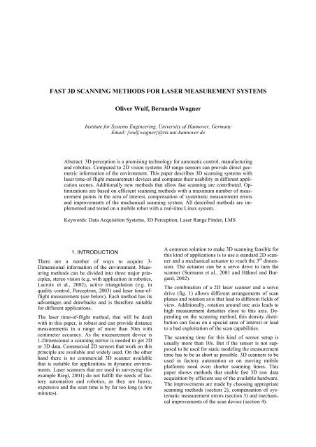
The combination of a 2D laser scanner and a servo
drive (fig. 1) allows different arrangements of scan
planes and rotation axis that lead to different fields of
view. Additionally, rotation around one axis leads to
high measurement densities close to this axis. Depending
on the scanning method, this density distribution
can focus on a special area of interest or lead
to a bad exploitation of the scan capabilities.
The scanning time for this kind of sensor setup is
usually more than 10s. But if the sensor is not supposed
to be used for static modeling the measurement
time has to be as short as possible. 3D scanners to be
used in factory automation or on moving mobile
platforms need even shorter scanning times. This
paper shows methods that enable fast 3D raw data
acquisition by efficient use of the available hardware.
The improvements are made by choosing appropriate
scanning methods (section 2), compensation of systematic
measurement errors (section 3) and mechanical
improvements of the scan device (section 4).

c)
Fig. 1. 3D scanner (yawing scan) consisting of a 2D laser
range sensor (Sick) and a servo drive (Powercube)
d)
2. SCANNING METHODS
An obvious optimization of the measurement system
is to take the scanning method that is most suitable
for the application. However, taking a 2D laser scanner
with 180° scanning range and a servo drive results
in a number of possible combinations of scan
planes and rotation axis to get a 3D scan. This section
describes four of these combinations. Subsection 2.1
gives a graphical analysis showing the measurement
density distributions. Based on this analysis and
experimental results the scanning methods are compared
in 2.2.
We have named the scanning methods as pitching
scan, rolling scan, yawing scan and yawing scan top.
The pitching scan (Fig. 2a) has a horizontal scan
plane and is pitching up and down. This method is
for example used in Surmann et al. (2001) and Hähnel
and Burgard (2002). A method that is newly
introduced here is the rolling scan (Fig. 2b). This
scan is rotating around the center of the scanner, with
the advantage of only one focus point in front of the
sensor. The yawing scan (Fig. 2c) and the yawing
scan top (Fig. 2d) have a vertical scan plane and are
rotating around the upright z-axis. This method is
used e.g. by Riegl (2001).
a)
b)
Fig. 2. Scanning schemes (left) and measurement density
distribution (right): (a) pitching scan, (b) rolling scan, (c)
yawing scan and (d) yawing scan top
2.1 Measurement density
As described above, variations of the rotation axis
and the alignment of the 2D scanner lead to a number
of different scanning patterns. On one hand these
scanning patterns differ in the field of view that can
be specified by a horizontal apex angel, a vertical
apex angel and the center of the scan. On the other
hand they differ in the distribution of the distance
measurements. Compared to a camera e.g. the measured
points are not placed in a regular grid. The rotation
of the 2D sensor leads to an accumulation of
scan points along the rotation axis that lead to a non
homogeneous measurement density distribution. The
measurement density is minimal for laser beams
orthogonal to the rotation axis and maximal for
beams parallel to this axis.
One possibility to illustrate the measurement density
distribution and the field of view, that is spanned by
the apex angles, is to show the measurement points
on a virtual sphere surrounding the 3D scanner. The
right column of figure 2 shows this method applied to
the described scanning patterns. It can be seen, for
example, that the pitching scan (fig. 2a) has got two
regions with a high measurement density on both
sides of the scanner and the rolling scan (fig. 2b) one
large region with a high density in front of the sensor.
These illustrations can be used for a qualitative comparison
of different scanning patterns.
2.2 Experimental comparison
This subsection shows experimental results of all
four scanning methods. The results illustrate the
meaning of the measurement density distribution in
real environments. Based on these results the practicability
in different applications is briefly discussed.
The examples are chosen from our mobile robotics
background, but similar scenarios can also be found
in other parts of flexible automation. Furthermore the

goal of this subsection is to illustrate the amount of
information and the potential that lies in 3D sensing.
The first experiment was made in a simple indoor
environment. It shows a person standing in the corridor
of our lab. Even though the scans shown in figure
3a and 3b took the same scanning time (1.6s), and
therefore consist of the same amount of points (about
22000), the scans are very different. It can be seen
that the measurement points are not uniformly distributed.
The pitching scan (fig. 3a) contains two
regions with a large number of points on the walls to
the left and the right side of the scanner, whereas the
person in front of the scanner is only sensed with a
few measurement points. On the other hand the rolling
scan (fig. 3b) centers most of its measurement
points in one region in front of the scanner and only a
few points along the walls on the side. Here, the
representation of the person in front of the sensor is
more detailed.
measured geometric information can be used directly
to estimate the container position, orientation and
height. The applicable scanning methods are also
depending on the required field of view. But in contrast
to the application in safety systems the rolling
scan might not be preferred to the pitching scan or
yawing scan. In measurement applications the regular
structure consisting of horizontal rows and vertical
columns might be easier to handle in following data
processing steps (segmentation, object detection).
Anyway the measurement points on the sides of the
scanner would be wasted in this case.
a)
a)
b)
b)
Fig. 3 Corridor with standing person: (a) pitching scan
(1.6s), (b) rolling scan (1.6s)
One possible application of 3D scanners is to build
up safety systems. These systems can be used for
area protection in factory automation, collision
avoidance on mobile robots or in surveillance. In this
applications the scanning method is first of all depending
on the needed field of view. For applications
with a horizontal apex angle of less then 180° the
pitching scan, the yawing scan or the rolling scan are
applicable, whereby the rolling scan has got the most
measurement points in the area of interest in front of
the sensor. In case that a larger apex angel is needed,
only the yawing scan and the yawing scan top are
applicable.
A more advanced application for 3D laser scanners is
a measurement system for object localization and
recognition. An example scan for this kind of application
can be seen in figure 4a showing a ramp and
two containers. In the top view calculated from the
same scan (fig. 4b) the different nature of 2D camera
pictures and 3D range scans becomes clear. The
Fig. 4 Position estimation of a ramp and 2 containers:
(a) pitching scan side view, (b) top view
Another, more specialized application for laser scanners
is mobile robot navigation in indoor environments,
including localization and mapping. There are
a number of solutions that manage this navigation
task by using 2D laser sensors and maps build of
simple features like lines or corners. These algorithms
work well under the condition that enough
straight wall segments can be seen. But this precondition
excludes packed rooms and environments with
many people. As walls in different heights and the
ceiling can be seen in 3D scans, the information
content of 3D scans offers a potential solution for
navigation problems in this kind of environments.
Figure 5a shows a yawing scan top of a packed room.
In contrast to the 2D scan taken in the same room
(fig. 5b), large parts of the walls and the ceiling can
be seen. In this special kind of application the yawing
scan top would be the most suitable scanning
method. With its 360° apex angle and perception of
the whole upper hemisphere, this scanning method
covers 100% of the area of interest in flat indoor
environments.

a)
b)
Fig. 5 3D scan for indoor navigation: (a) yawing scan top
(2.8s), (b) 2D scan of the same room
To complete the list of scanning methods, the experiments
that can be seen in figure 6a and 6b show
3D scans measured with the yawing scan method.
The advantage of this scanning method is that it is
possible to make scans with a horizontal apex angel
larger than 180°. This wide opening angle is for example
useful in outdoor navigation of mobile robots.
a)
b)
Fig. 6 Yawing scan (270°, 4s) in outdoor application:
(a) avenue (b) car park
3. SYSTEMATIC MEASUREMENT ERRORS
The analysis of systematic measurement errors and
the compensation of these effects play an important
role in 3D scanning. Here the synchronization of the
laser device and the position of the servo drive have a
major influence on the accuracy of the 3D point
cloud, as it is already mentioned in Herbert and
Krotkov (1991). Especially fast scanning is effected
by poor synchronization, as it can be seen in the
following example: A 3D scanning device with the
commonly used Sick LMS 200 and a 1° resolution
results in a rotation speed ω s = 75° / s of the servo
drive. The maximum systematic measurement error
e due to a miss synchronization of ∆ t = 100ms
and
an object distance of d = 10m
can be estimated as
follows:
( ⋅ t)
e = d ⋅sin ωs ∆
(3.1)
resulting in a maximal systematic measurement error
with a magnitude of e = 1. 3m
for a typical non realtime
system.
Subsection 3.1 describes a real-time implementation
and a method to build time consistent data sets. Subsection
3.2 describes how the Sick LMS 200 creates
its 0.5° resolution. The understanding of this function
leads to better time correlation and therefore better
accuracy.
3.1 Time-consistent data sets
A common representation for 3D measurements is
the 3D point cloud given in Cartesian coordinates (as
seen in fig. 3 – 6). To calculate this 3D point cloud a
transformation is needed that has the 2D raw scan
and the position of the 2D scanner as its inputs. As it
was already stated in the beginning of this section, it
is important that the scanner position at the time of
the scan is known. This means that a time consistent
data set, consisting of a laser scan and the servo drive
position is needed.
One way to get this data set is a sequential data capturing
procedure that waits for a new laser scan and
reads the servo drive position afterwards. The problem
with this simple procedure is that the acquired
data set is not time consistent. In this case the servo
drive position is not specifying the scanner position
at the time of the scan, but its position a short time
after. This “short” time is system dependent and can
be up to several 100 ms due to a servo drive that
gives only time discrete response or a non real-time
OS that is delayed by hard disk I/O or memory arrangements.
A possibility to overcome this problem is a different
data capturing procedure for real-time operating
systems. This data acquisition system consists of
three tasks. Two of these tasks read continuous data
from the laser scanner and the servo drive, where
these tasks must neither be synchronized nor have the
same sampling frequency (fig. 7). The correlation is
made subsequently based on accurate timestamps
that are attached to each raw data sample. The third
task connects this raw data to get a time consistent
data set and to calculate the transformation into Cartesian
coordinates. As this calculation is only based
on the given timestamps, the third task is not time
critical and can be performed with low priority, remote
or even offline without loss of precision.
Given the accurate timestamps, the actual assembly
procedure is fairly easy. The third task waits for a
new 2D laser data package and looks up the accord-

ing position in a list of received servo drive positions.
Because the position at the accurate scan time is not
generally given, the position can be linearly interpolated
between the two closest servo drive positions
(fig. 7). For efficient calculation our actual implementation
is representing a 2D laser scan by a single
timestamp which leads to a maximal miss synchronization
of ∆ t = 3. 3ms
for the measured points at the
beginning and the end of the scan. For slower 2D
scanners (longer ∆ t ) or faster 3D scans (larger ω S ),
it might be necessary to represent the 2D scans with
start- and end-timestamps and to interpolate the laser
measurement point of time as well.
resulting in an angle resolution of ∆ϕ = 1°
for the
scanner with f L = 27kHz
sampling rate and a rotation
speed of ωm = 75⋅
2π
/ s (13.3ms turnaround
time). If the maximum sampling rate is fixed an angular
resolution of 0.5° or 0.25° can be reached in
two different ways. One possibility is, according to
equation 3.2, a lower mirror speed, resulting in a turn
around time of 26.6ms for 0.5° and 53.3ms for 0.25°
resolution. The second possibility, which is applied
in the sick sensor, is to assemble the 0.5° scan out of
two scans with 1° resolution. Here, the mirror is
constantly rotating with a speed of ωm = 75⋅
2π
/ s
and is measuring the first scan with 1° resolution and
0° offset and the second scan also with a resolution
of 1° but an offset of 0.5° (Fig. 8). Similarly the
0.25° resolution takes four turns with 0.0°, 0.5°,
0.25° and 0.75° offsets. This scanning pattern does
not affect the scanning time or the accuracy of static
scans but it disturbs fast 3D scan, as an exact measurement
timestamp cannot be given. For this case the
Sick raw data mode offers a good solution. This
measuring mode uses the same scanning pattern to
generate the 0.5° resolution but in contrast to the
standard mode, which measures two turns and transmits
a 0.5° data package thereafter, the raw data
mode transmits two 1° data packages directly after
the measurement. This allows more accurate timestamps
and therefore better compensation of systematic
measurement errors.
Fig. 7. Synchronization of laser scanner and servo drive
Fig. 8. Sick LMS Raw Data Mode
3.2 Sick LMS Raw Data Mode
To assign accurate timestamps and to compensate
systematic measurement errors, knowledge about the
measurement principle and the actual implementation
of the sensor is needed. As the implementation is
sensor dependent, this paper takes the LMS 200 series
of the company Sick as an example. This 2D
laser range scanner is a standard industrial product
which is widely used in robotics.
The Sick 2D scanner, similarly to other sensors,
consists of a 1D laser range measurement device and
a continuously rotating mirror. The 180° opening
angle of the sensor is separating the measurement
stream into two equal sized time slots. One measurement
slot and one slot where no measurements are
possible because the mirror is facing the inside of the
case. This timeslot is used for communication and
data transfer. The angle resolution ∆ ϕ can be calculated
from the sampling rate f L and the rotation
speed of the mirror ω as follows:
m
ωm
∆ ϕ =
(3.2)
f
L
4. CONTINUOUS SCANNING
All 3D scans that have been presented in this paper
so far and all publications concerning 3D scanners
consisting of a 2D laser scanner and an extra servo
drive use a servo drive with limited turning circle.
This limitation is due to the cable connections of the
laser sensor for power supply and data transfer. The
problem of the limited turning circle is that the scanner
cannot be turned with constant speed. The sensor
has to be accelerated at the start and the end of each
turn. This accelerations can lead to mechanical problems
especially on fast scans. On one hand the lifetime
and mechanical stability of the sensor is reduced
due to the forces that come with the positive and
negative acceleration, on the other hand the servo
drive has to be more powerful and requires more
energy compared to a continuously moving scanner,
a drawback especially on mobile systems.
Fig. 9. Scan drive prototype with
IBEO 2D range finder
A solution for this problem, that has been build as a
prototype (fig. 9) at the institute, is a 3D scanner with
a continuously moving servo drive. To enable this
endless turning, it is necessary to replace the cable
connections for power and data transfer by slip rings.
For this reason the implemented prototype has got a 4
pole slip ring with 2 poles for 24V power supply and
2 poles for data transfer via 1Mbit CAN bus.

Fig. 10. Range image taken with the
continuously turning 3D scanner
Riegl Laser Measurement Systems (2001). Data
sheet, LMS-Z210, www.riegl.com
Sick AG (2000). Data sheet, LMS 200,
www.sick.com
Surmann, H., K. Lingemann, A. Nüchter and J.
Hertzberg (2001). A 3D Laser Range Finder for
Autonomous Mobile Robots, In: Proceedings of the
International Symposium on Robotics, Zurich, Switzerland
5. CONCLUSION
This paper described a sensor system that is able to
acquire 3D geometric information of the environment.
The system consists of a 2D laser range sensor
working on the time-of-flight measurement principle,
a servo drive as mechanical actuator and a processing
unit that collects raw data and calculates point clouds
in Cartesian space.
The focus of this paper lies on the fast acquisition of
undistorted raw data that allows the use of 3D sensors
in safety systems, factory automation and on
moving platforms like service robots. All scanning
3D sensors that are available at present can only be
used for static modeling as the measurement of one
scan takes several minutes. Even the 3D scanners that
are used on mobile robots need more than 10s to take
a single scan with an apex angle of 180 ° × 90°
.
This paper described improvements that allow fast
scanning. The contributions are made by laying a
focus on the measurement density distribution, by
compensation of systematic measurement errors and
by mechanical improvements of the scanning device.
These improvements allow fast scanning with scan
times from 1.6s for an apex angle of 180 ° × 180°
to 5
seconds for 360 ° × 180°
without distortion. The only
limiting factor at this moment is the maximum measurement
rate of the available 2D scanners. Thus the
scanner can be used in dynamic environments and
not only for static modeling.
REFERENCES
Hähnel, D. and W. Burgard (2002). Map Building
with Mobile Robots in Populated Environments, In:
Proceedings of the International conference on Intelligent
Robots and Systems, Lausanne, Switzerland
Herbert, M. and E. Krotkov (1991). 3-D Measurements
from Imaging Laser Radars: How good are
they?, In: Proceedings of the International Workshop
on Intelligent Robots and Systems, Osaka, Japan
Lacroix, S., A. Mallet, D. Bonnafous, G. Bauzil, S.
Fleury, M. Herrb and R. Chatila (2002). Autonomous
Rover Navigation on Uneven Terrains: Functions
and Integration, International Journal of Robotics
Research, Volume No 21, pp. 917 - 942
Perceptron (2003). ScanWorks 3D product Brochure,
www.perceptron.com