Chapter 6. Advanced Data Structures (Search Trees)

6. Elementary Data Structures 6-1
Chapter 6. Advanced Data Structures (Search Trees)
Balanced Binary Search Trees [S, Ü11.2]
Worst-case running time for BST is ¢´µ ¢´Òµ.
Đ Can be improved to ¢´ÐÓ Òµ if we can guarantee that ¢´ÐÓ Òµ—balanced BST.
Idea: restructure tree if necessary (when insert or delete) to balance its height.
Ð Methods: AVL tree, 2-3 tree, red-black tree, B tree, etc.
Recall that a set Ë has many different BST representations.
Let ´Ì µ denote the height of a BST Ì , with subtrees Ì Ð and Ì Ö , and assume that if Ì is empty
then ´Ì µ ½.
Definition 1
Ì is height balanced of degree k, denoted HB(), if
(1) ´Ì Ð µ ´Ì Ö µ , and
(2) Ì Ð and Ì Ö are HB().
Definition 2
Ì is height balanced, denoted HB, if it is HB(1).
Definition 3
The balance factor of Ì is defined as
´Ì µ ´Ì Ð µ ´Ì Ö µ
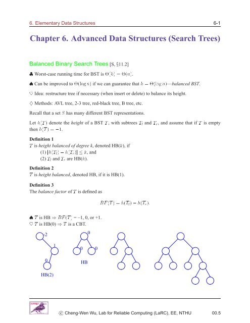
Đ Ì is HB µ ´Ì µ = –1, 0, or +1.
Ì is HB(0) µ Ì is a CBT.
-2
0
1
0
0
0
HB
HB(2)
c­ Cheng-Wen Wu, Lab for Reliable Computing (LaRC), EE, NTHU 00.5

6. Elementary Data Structures 6-2
AVL Tree [S, Ü11.2]
Definition 4 (Adelson/Velskii/Landis)
An empty BST is an AVL tree. If Ì is a nonempty BST with Ì Ð and Ì Ö as its left and right subtrees,
then Ì is an AVL tree iff
1) Ì Ð and Ì Ö are AVL trees, and
2) ´Ì Ð µ ´Ì Ö µ ½.
HB BST AVL tree
Theorem 1
The height of an AVL tree Ì with Ò nodes satisfies
That is, ´Ì µ Ç´ÐÓ Òµ.
´Ì µ ½ ÐÓ Ò
Proof :LetÆ be the minimum number of nodes in an AVL tree Ì with height . Then
Æ ¼ ½
Æ ½ ¾ and
Æ Æ ½ · Æ ¾ · ½ ¾
It can be verified easily (by induction) that
Therefore,
Ô
ÐÓ´
Ò ·¾ ½
Æ ·¾ ½
Ô
Ô
Ô
½
´ ½ ·
µ ·¾ ´ ½
µ ·¾ ℄ ½
¾
¾
Ô
Ô
½
´ ½ ·
µ ·¾ for large
¾
Òµ ´ · ¾µ ÐÓ´ ½ · Ô
µ ÐÓ Ò Ô
· ÐÓ
ÐÓ ½½
½ ÐÓ Ò
As an example, we insert 10, 6, 2, 3, 11, 7, 9, 8, 1, 5, 4 into an empty BST and keep it HB. The
final tree is an AVL tree:
¾
¾
µ
¾
c­ Cheng-Wen Wu, Lab for Reliable Computing (LaRC), EE, NTHU 00.5

6. Elementary Data Structures 6-3
10:
10
6:
10
2:
2
10
6
HB
6
HB
0
1
6
2
not HB
rotate right
µ
2
HB
10
3:
6
11:
6
7:
6
9:
6
2
10
2
10
2
10
2
10
8:
2
3
HB
6
10
3 7 11
µ
3
HB
2
11
3
6
10
8 11
3 7 11
HB
1, 5, 4
...
1
2
4
6
3 7 11
9
HB
10
8 11
9
7
9
3
5
7
9
not HB 8
HB
Definition 5
An AVL tree Ì is balanced if ´Ì Ð µ ´Ì Ö µ. Ì is right heavy if ´Ì Ö µ ´Ì Ð µ·½. Ì is left heavy
if ´Ì Ð µ ´Ì Ö µ · ½.
=
/
· ½
balanced
right heavy
left heavy
typedef struct node{
char CC; /* condition code */
int key;
struct node *left, *right;
} NODETYPE, *NODEPTR;
c­ Cheng-Wen Wu, Lab for Reliable Computing (LaRC), EE, NTHU 00.5

6. Elementary Data Structures 6-4
On the insertion path of an element from root to leaf:
Ü
Ü
Ü
Ü
Ü
=
Ü Ü Ü
No change in AVL property. No change.
(But CC will change.)
Ü
No change.
Ü
Needs balancing.
Ü
Needs balancing.
Exercise 1
Give the CC of each of the nodes in the following AVL tree.
8
1
3
6
11
21
23
2
5
7
10
16
22
25
4
9
13
18
24
12
14
17
19
¾
c­ Cheng-Wen Wu, Lab for Reliable Computing (LaRC), EE, NTHU 00.5

6. Elementary Data Structures 6-5
Balancing AVL Tree
Assume before insertion of Ü, tree Ì was HB(1).
(1) Single left rotation (SLR): to change old CCs on the path, we go from leaf up. We find CC =
right-heavy, then rotate at that point.
T1
A
T2
B
T3
x
SLR
µ
T1
A
T2
B
T3
x
(2) Single right rotation (SRR): to change old CCs on the path, we go from leaf up. We find CC =
left-heavy, then rotate at that point.
T1
x
A
T2
B
T3
SRR
µ
T1
x
A
T2
B
T3
Rules: (a) Go up from left till left-heavy found. (b) Go up from right till right-heavy found.
c­ Cheng-Wen Wu, Lab for Reliable Computing (LaRC), EE, NTHU 00.5

6. Elementary Data Structures 6-6
(3) Double right rotation (DRR)
A
B
C
µ
DRR
A
B
C
T1
T2
x
or
T3
x
T4
T1
T2 T3
x x
Height remains the same.
T4
(4) Double left rotation (DLR)
T1
T2
x
A
B
or
T3
x
C
T4
µ
DLR
T1
B
A
C
T2 T3
x x
Height remains the same.
T4
¯ Must check that BST properties are maintained.
Stack of CCs: We maintain a stack of CCs for each insert operation.
Exercise 2
Insert 20 into the AVL tree of the previous example. Set up the stack when the inserted item is
being pushed along the inserting path.
¾
Going from the insertion point (leaf) up to the root, let current be the node currently being
scanned, with child and gchild.
child = node inserted; gchild = NULL; /* initial condition */
hc = CC = condition code;
if(hc(current) == ‘=’)
if(child == rchild(current)) hc(current) = ‘\’; /* from right */
else hc(current) = ‘/’; /* coming from left */
c­ Cheng-Wen Wu, Lab for Reliable Computing (LaRC), EE, NTHU 00.5

6. Elementary Data Structures 6-7
gchild = child;
child = current;
current = pop(stack);
if((hc(current) == ‘/’ && child == rchild(current)) ||
(hc(current) == ‘\’ && child == lchild(current)))
{ hc(current) = ‘=’; return; }
else rebalance the tree @ current;
AVL Tree Deletion
Assume the deleted node is a leaf.
Đ Use a stack.
I.C.: child is the deleted node, and current is its parent.
We use a bottom-up strategy:
1. if(hc(current) == ‘=’)
{ if(child == lchild(current)) hc(current) = ‘\’;
else hc(current) = ‘/’;
return;
}
2. if((hc(current) == ‘/’ && child == lchild(current)) ||
(hc(current) == ‘\’ && child == rchild(current)))
{ hc(current) = ‘=’;
child = current;
current = pop(stack);
}
3. else
{ rebalance @ current;
child = current;
current = pop(stack);
}
Exercise 3
(a) We showed in Chapter 4 that every comparison based algorithm to sort Ò elements must take
Ç´Ò ÐÓ Òµ time in the worst case. What implication does this result have on the complexity of
initializing an AVL tree of Ò nodes?
(b) Write an algorithm to list the nodes of an AVL tree Ì in ascending order of Ý. Can this be
done in Ç´Òµ time if Ì has Ò nodes?
c­ Cheng-Wen Wu, Lab for Reliable Computing (LaRC), EE, NTHU 00.5

6. Elementary Data Structures 6-8
(c) How do you combine two AVL trees into a bigger new AVL tree? Can this be done in linear
time?
¾
2-3 Tree
Definition 6
A 2-3 tree is a search tree that is either empty or satisfies the following properties:
1. Each internal node is either a 2-node (with 2 children) or a 3-node (with 3 children). A
2-node has one element; a 3-node has two elements.
2. All elements in the 2-3 subtree with root lchild have key less than lkey.
3. All elements in the 2-3 subtree with root mchild have key greater than lkey (and less than
rkey if it is a 3-node).
4. If it is a 3-node, then all elements in the 2-3 subtree with root rchild have key greater than
rkey.
5. All external nodes are at the same level, i.e. Ì is HB.
6. All the elements appear at the leaves (external nodes).
typedef struct NODE *NODEPTR;
struct NODE {
int lkey, rkey;
NODEPTR lchild, mchild, rchild;
};
search(NODEPTR T, int x)
{
while(T)
switch(compare(x,T))
{
case 1: T = T->lchild; break;
case 2: T = T->mchild; break;
case 3: T = T->rchild; break;
case 4: return T;
}
return NULL;
}
c­ Cheng-Wen Wu, Lab for Reliable Computing (LaRC), EE, NTHU 00.5

6. Elementary Data Structures 6-9
40
+
11
+
10 20
80
+
7
9
15
+
5 10 20 40 80 2 7 9 11 15
Exercise 4
Write the compare function used in the above procedure.
¾
Exercise 5
(a) Show that a 2-3 tree has height which satisfies
ÐÓ ¿
Ò ÐÓ ¾
Ò
(b) Show that searching can be done in Ç´ÐÓ Òµ time.
¾
Insertion:
insert(T, y) NODEPTR T; int y; [cf. HSA, Sec. 10.3.3]
{ NODETYPE p, q;
if(!(*T)) new_root(T, y, NULL); /* T was empty */
else
{ p = find_node(*T, y); /* Is y in T? */
if(!p) /* y is in T */
{ fprintf(stderr, "The key is currently in T.\n");
exit(1);
} /* else get to the node where y is to be inserted */
q = NULL; /* q will be the newly created node after split */
for(;;)
if(p->rkey == INFINITY) /* p is a 2-node */
{ put_in(&p, y, q); /* insert y into p and place q */
break; /* immediately to the right of y */
}
else /* p is a 3-node */
{ split(p, &y, &q);
if(p == *T) /* split the root; h = h+1 */
{ new_root(T, y, q); /* create new node q */
break;
c­ Cheng-Wen Wu, Lab for Reliable Computing (LaRC), EE, NTHU 00.5

6. Elementary Data Structures 6-10
}
}
}
}
else p = pop(stack); /* follow the path back up */
split(p, yp, qp) NODETYPE p; NODEPTR yp, qp;
{ take node p with 2 keys in it;
create a new node q with q.lkey = max(p.rkey, y);
and q.rkey = INFINITY;
temp = median(p.lkey, p.rkey, y);
p.lkey = min(p.lkey, y);
y = temp; /* the median key sent upward */
update the pointers;
}
40
+
insert(T, 70):
40
+
insert(T, 30):
20 40
10 20
80
+
10 20
70 80
10
+
30
+
70 80
5
10
20
40
80
5
10
20
40
70 80
5
10
20
30
40
70 80
Exercise 6
What is the result of a subsequent insert(T, 60)?
¾
Deletion:
modify p as necessary to reflect status after element has been deleted;
while(p has 0 element && p is not root)
{ r = parent of p;
q = left or right sibling of p (as appropriate);
if(q is a 3-node) rotate;
else combine;
p = r;
}
if(p has 0 element) /* then p must be the root */
{ left child of p becomes the new root;
delete p;
}
c­ Cheng-Wen Wu, Lab for Reliable Computing (LaRC), EE, NTHU 00.5

6. Elementary Data Structures 6-11
Exercise 7
(a) We showed in Chapter 4 that every comparison based algorithm to sort Ò elements must take
Ç´Ò ÐÓ Òµ time in the worst case. What implication does this result have on the complexity of
initializing a 2-3 tree of Ò nodes?
(b) Write an algorithm to list the nodes of an 2-3 tree Ì in ascending order of Ý. Can this be
done in Ç´Òµ time if Ì has Ò nodes?
(c) How do you combine two 2-3 trees into a bigger new 2-3 tree? Can this be done in linear time?
¾
2-3-4 Tree
A 2-3-4 tree extends a 2-3 tree so that 4-nodes are also permitted (4-nodes may have up to 4
children).
typedef struct NODE *NODEPTR;
struct NODE {
int lkey, mkey, rkey;
NODEPTR lchild, lmchild, rmchild, rchild;
};
50
10
70 80
5
7
9
30 40
60
75
85 90 92
Đ The height of a 2-3-4 tree with Ò elements is between ÐÓ ´Ò · ½µ and ÐÓ ¾´Ò · ½µ.
An advantage 2-3-4 trees have over 2-3 trees is that insertion and deletion can be done by a
single root to leaf pass.
We can efficiently represent a 2-3-4 tree as a BST called red-black tree (see next section), which
utilizes space more efficiently than a 2-3 or 2-3-4 tree.
c­ Cheng-Wen Wu, Lab for Reliable Computing (LaRC), EE, NTHU 00.5

6. Elementary Data Structures 6-12
Insertion: To avoid the backward leaf to root pass, we split 4-nodes on the way down the tree to
the leaf node into which the element is to be inserted (see Figs. 10.21-24, pp. 512-514). The leaf
node which the insertion is to be made is therefore guaranteed to be a 2- or 3-node. No further
node splitting is required.
Deletion: To avoid the backward leaf to root restructuring path, it is necessary to ensure that at
the time of deletion, the element to be deleted is in a 3- or 4-node. This is accomplished by
restructuring the 2-3-4 tree during the downward root to leaf pass (see Fig. 10.25, p. 517).
Exercise 8
Show that insertion and deletion can be done in Ç´ÐÓ Òµ time.
¾
Red-Black Tree [S, Ü11.3]
A red-black tree is a BST representation of a 2-3-4 tree, in which every node (pointer) is colored
either red or black.
typedef enum {red,black} color;
typedef struct NODE *NODEPTR;
typedef struct NODE {
int key;
NODEPTR lchild, rchild;
color lcolor, rcolor;
};
☞ If the child pointer was present in the original 2-3-4 tree, it is a black pointer. Otherwise, it
is a red pointer.
☞ An alternative node structure in which each node has a single color field may also be used,
whose value is the color of the pointer from the node’s parent.
☞ The root node is a black node by definition.
☞ All external nodes are black nodes, too.
Transformation from a 2-3-4 tree to a red-black tree:
1. A 2-node Ô is represented by a node Õ with both its color fields black, key = lkey, q-
>lchild = p->lchild,andq->rchild = p->lmchild.
2. A 3-node is represented by two nodes connected by a red pointer.
c­ Cheng-Wen Wu, Lab for Reliable Computing (LaRC), EE, NTHU 00.5

6. Elementary Data Structures 6-13
3. A 4-node is represented by three nodes one of which is connected to the remaining two by
red pointers.
The above 2-3-4 tree example is transformed into the following red-black tree.
50
10
70
7
40
60
80
5
9
30
75
90
85
92
From the transformation rules we can show that a BT is a red-black tree iff it satisfies the
following properties:
¯ It is a BST.
¯ Every root to external node path has the same number of black pointers (since all external
nodes of the original 2-3-4 tree are on the same level).
¯ No root to external node path has 2 or more consecutive red pointers.
☞ Every red-black tree with Ò nodes has a height ¾ÐÓ ¾´Ò · ½µ.
☞ Read Ü11.3 [S] for details of insertion & deletion.
Exercise 9
Compare the worst-case height of a red-black tree with Ò nodes and that of an AVL tree with the
same number of nodes.
¾
Multiway Search Tree [S, Ü11.4]
Definition 7
A multiway search tree of order Ò (or Ò-way search tree) is a generalization of 2-3 tree, in which
each node has Ò or fewer subtrees and contains one fewer keys than it has subtrees; each of the
subtrees can be empty; and empty subtrees are not necessarily on the right.
c­ Cheng-Wen Wu, Lab for Reliable Computing (LaRC), EE, NTHU 00.5

6. Elementary Data Structures 6-14
1. Ì is an AVL tree µ Ì is a 2-way search tree.
2. Ì is a 2-3 tree µ Ì is a 3-way search tree.
3. Ì is a 2-3-4 tree µ Ì is a 4-way search tree.
Nodes as full as possible µ as less storage wasted as possible (keep as many keys as possible in
each node).
Example 1
Let there be 4000 elements (keys). If Ò then we have 1000 nodes of 4 keys each, so . If
Ò ½½ then we have 400 nodes of 10 keys each, so ¿.
For full nodes, they use about the same amount of storage.
Accessing a node is the most expensive operation in searching external storage, where multiway
trees are used most often.
¾
B-Tree [S, Ü11.4]
Definition 8
A B-tree of order m is a balanced order-Ñ multiway search tree in which 1) each non-root internal
node contains Ò¾ keys; 2) the root node has at least 2 children; and 3) all external nodes are
at the same level.
☞ A.k.a. ´Ñ ½µ-Ñ tree.
☞ Each node has a maximum of Ñ
½ keys and Ñ children.
☞ They are good at minimizing disk I/O operations.
☞ The height of Ì is Ç´ÐÓ Ñ¾´Ò¾µµ.
☞ Read Ü11.4 [S] for details of insertion & deletion.
Trie
A trie is a tree of degree ¾ in which the branching at any level is determined not by the entire
key value but by only a portion of it. Its internal nodes are branch nodes (which contain pointers
only) and external nodes are element nodes.
c­ Cheng-Wen Wu, Lab for Reliable Computing (LaRC), EE, NTHU 00.5

6. Elementary Data Structures 6-15
#define MAXLETTER 27 /* blank + 26 letters */
#define MAXCHAR 30 /* max length of key */
typedef enum {key,pointer} nodetype;
typedef struct NODE *NODEPTR;
struct NODE {
nodetype tag;
union {
int *key;
NODEPTR letter[MAXLETTER];
} u;
};
NODEPTR root;
search(NODEPTR T, int *key, int i)
{
if(!T) return NULL; /* not found */
if(T->tag == key)
return ((strcmp(T->u.key, key))? NULL : T);
return search(T->u.letter[get_index(key,i)], key, i+1);
}
c­ Cheng-Wen Wu, Lab for Reliable Computing (LaRC), EE, NTHU 00.5