Classification of Cervical Cancer Cells Using HMLP ... - AU Journal
Classification of Cervical Cancer Cells Using HMLP ... - AU Journal
Classification of Cervical Cancer Cells Using HMLP ... - AU Journal

Create successful ePaper yourself
Turn your PDF publications into a flip-book with our unique Google optimized e-Paper software.
<strong>Classification</strong> <strong>of</strong> <strong>Cervical</strong> <strong>Cancer</strong> <strong>Cells</strong> <strong>Using</strong><br />
<strong>HMLP</strong> Network with Confidence Percentage and<br />
Confidence Level Analysis.<br />
N. A. Mat-Isa 1 , M. Y. Mashor 2 , N. H. Othman 3<br />
1,2<br />
Control and Electronic Intelligent System (CELIS) Research Group,<br />
School <strong>of</strong> Electrical & Electronic Engineering,<br />
Universiti Sains Malaysia,Malaysia<br />
1 E-mail: ashidi75@yahoo.co.uk<br />
2 E-mail: yus<strong>of</strong>@eng.usm.my<br />
3 Pathology Department, School <strong>of</strong> Medical Science<br />
Universiti Sains Malaysia, Malaysia.<br />
E-mail: hayati@kb.usm.my<br />
Abstract<br />
In most previous studies, the analysis on<br />
the ability <strong>of</strong> neural networks to be used as a<br />
good cervical cancer diagnosis technique is<br />
only based on accuracy, sensitivity,<br />
specificity, false negative and false positive.<br />
In the current study, we go one step further<br />
by introducing analysis <strong>of</strong> diagnosis<br />
confidence percentage and diagnosis<br />
confidence level to analyse the ability <strong>of</strong><br />
neural network to produce a good diagnosis<br />
performance. The current study used hybrid<br />
multilayered perceptron (<strong>HMLP</strong>) network to<br />
diagnose cervical cancer in the early stage<br />
by classifying cervical cells into normal,<br />
LSIL and HSIL cell. The proposed diagnosis<br />
confidence percentage and diagnosis<br />
confidence level analysis have been proved<br />
to give clearer picture on the strength or<br />
confidence level <strong>of</strong> each diagnosis, which is<br />
done by <strong>HMLP</strong> network.<br />
Keywords<br />
<strong>Cervical</strong> cancer, <strong>HMLP</strong> network,<br />
diagnosis confidence percentage, diagnosis<br />
confidence level, Pap test.<br />
1. Introduction<br />
<strong>Cervical</strong> cancer is the second common<br />
malignancy in women. However, in<br />
Malaysia, Ministry <strong>of</strong> Health reported<br />
cervical cancer is the first leading cancers in<br />
women (Ministry <strong>of</strong> Health, 1999).<br />
Malaysian government has launched the<br />
National <strong>Cancer</strong> Control Program to reduce<br />
International <strong>Journal</strong> <strong>of</strong> The Computer, The Internet and Management, Vol. 11, No.1, 2003, pp. 17 - 29<br />
17
N. A. Mat-Isa, M. Y. Mashor, N. H. Othman<br />
the incidence and mortality <strong>of</strong> cancer<br />
including cervical cancer. The program aims<br />
to improve the quality <strong>of</strong> life <strong>of</strong> cancer<br />
patients. The program policies encompass<br />
prevention, early diagnosis, treatment,<br />
palliative care and rehabilitation. In order to<br />
reduce the incidence and mortality <strong>of</strong><br />
cervical cancer, the program aims to increase<br />
the Pap test facilities and public education<br />
campaign.<br />
In Malaysia, Papanicolaou test or better<br />
known as Pap test is commonly used as<br />
cervical cancer screening test. Several<br />
previous studies by Breen et al. (2001),<br />
Framer (2001), Kuie (1996) and Adami et al.<br />
(1994), showed that the chances for a woman<br />
<strong>of</strong> acquiring cervical cancer is reduced as she<br />
has Pap test regularly. However, studies by<br />
Othman et al., (1997, 1995), Kuie (1996) and<br />
Hislop et al. (1994) proved that sometimes<br />
the Pap test is not effective. The<br />
determination <strong>of</strong> abnormal cervical cells can<br />
sometimes be missed in certain situation.<br />
Three major reasons that decrease the<br />
accuracy <strong>of</strong> Pap test diagnosis result are bad<br />
Pap smear samples, technical errors and<br />
small size <strong>of</strong> CIN. Beside that, the screening<br />
procedure on the Pap smear sample requires<br />
an experienced pathologist and thus<br />
expensive and time-consuming.<br />
Due to the problems, several previous<br />
studies have successfully developed<br />
automated and semi-automated screening<br />
systems in order to increase the diagnosis<br />
performance <strong>of</strong> Pap test. Three<br />
supplementary diagnosis systems for Pap test<br />
which are commonly used in medical field<br />
and currently approved by the Food and<br />
Drug Administration (FDA) are Papnet,<br />
AutoPap and ThinPrep (WebMD, 2002,<br />
HTAC, 2002). Beside those supplementary<br />
systems, several previous studies also<br />
proposed artificial intelligence as a cervical<br />
cancer diagnosis system. The most popular<br />
artificial intelligence systems that were used<br />
for that purpose are neural networks.<br />
Multilayered perceptron network (MLP)<br />
becomes the most popular neural networks to<br />
be used as cervical cancer diagnosis system<br />
(Li & Najarian, 2001, Mitra et al., 2000,<br />
Balasubramaniam et al. 1998). Papnet<br />
system also used MLP network trained using<br />
back propagation (BP) algorithm. In the<br />
current study, <strong>HMLP</strong> network trained using<br />
modified recursive prediction error (MRPE)<br />
algorithm is proposed to diagnose cervical<br />
cancer.<br />
In almost all previous studies (eg. by<br />
Mat-Isa et al., 2002, 2001, Li & Najarian,<br />
2001, Mitra et al., 2000) analyse to<br />
determine the ability <strong>of</strong> the neural networks<br />
to diagnose cervical cancer were only done<br />
based on accuracy, sensitivity, specificity,<br />
false negative and false positive. The current<br />
study goes one step further by introducing<br />
analysis <strong>of</strong> confidence percentage and<br />
confidence level to analyse the degree <strong>of</strong><br />
suitability <strong>of</strong> the <strong>HMLP</strong> network to be used<br />
as a cervical cancer diagnosis technique.<br />
2. Hybrid Multilayered Perceptron<br />
Network<br />
MLP network is a highly nonlinear<br />
neural networks. By using the MLP network,<br />
a linear system has to be approximated using<br />
the nonlinear neural network model.<br />
However, modelling a linear system using a<br />
nonlinear model can never be better than<br />
using a linear model. Therefore, Mashor in<br />
2000, proposed additional linear input<br />
connections to the MLP network. The<br />
modified version <strong>of</strong> MLP is called hybrid<br />
multilayered perceptron (<strong>HMLP</strong>) network.<br />
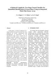
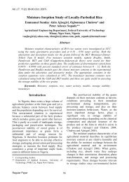
As shown in Figure 1, the <strong>HMLP</strong> network<br />
allows the network inputs to be connected<br />
directly to the output nodes via weighted<br />
connections to form a linear model, which is<br />
in parallel with the nonlinear original MLP<br />
model.<br />
18
Figure 1: One-hidden layer <strong>HMLP</strong> network.<br />
As shown in Figure 1, for the <strong>HMLP</strong><br />
network with m output nodes, n h hidden<br />
nodes and n i input nodes, the output <strong>of</strong> the<br />
kth neuron, y k , in the output layer is given<br />
by:<br />
yˆ<br />
( t)<br />
=<br />
k<br />
n<br />
n<br />
2<br />
w<br />
⎜<br />
jkF<br />
j= 1 i=<br />
1<br />
∑<br />
⎛<br />
⎝<br />
∑<br />
⎞<br />
⎟ +<br />
⎠<br />
∑<br />
h i n i<br />
w x ( t)<br />
+ b<br />
1 0<br />
ij i<br />
1<br />
j<br />
i=<br />
1<br />
w x ( t)<br />
for 1 ≤ k ≤ m<br />
(1)<br />
w ij<br />
w jk<br />
w ik<br />
1 2<br />
l<br />
where , and denote the<br />
weights <strong>of</strong> the connection between input and<br />
hidden layer, weights <strong>of</strong> the connection<br />
between hidden and output layer, and<br />
weights <strong>of</strong> the linear connection between<br />
1<br />
input and output layer respectively. b and<br />
x i<br />
denote the thresholds in hidden nodes and<br />
inputs that are supplied to the input layer<br />
respectively. F(•<br />
) is an activation function<br />
and is normally be selected as sigmoid<br />
function.<br />
l<br />
ik<br />
0<br />
i<br />
j<br />
From Equation (1), the values <strong>of</strong><br />
1 2 l<br />
1<br />
w<br />
ij<br />
, w<br />
jk<br />
, wik<br />
and b j<br />
must be determined<br />
using appropriate algorithm. BP algorithm is<br />
commonly used to find optimum values for<br />
those parameters. Although the algorithm is<br />
easy to be implemented and produces a good<br />
performance, but its convergence rate is<br />
slow. To overcome the problems, Chen et al.<br />
(1990) proposed recursive prediction error<br />
(RPE) to replace the BP algorithm. The RPE<br />
algorithm provides a faster convergence rate<br />
and better final convergence values <strong>of</strong><br />
weights and thresholds. In 2000, Mashor<br />
proposed a modified version <strong>of</strong> RPE<br />
algorithm, known as modified recursive<br />
prediction error (MRPE). By optimising the<br />
way the momentum and the learning rate are<br />
assigned, the MRPE algorithm is able to<br />
improve the convergence rate <strong>of</strong> the RPE<br />
algorithm. From the above discussion, the<br />
MRPE algorithm will be used to train the<br />
<strong>HMLP</strong> network in the current study.<br />
International <strong>Journal</strong> <strong>of</strong> The Computer, The Internet and Management, Vol. 11, No.1, 2003, pp. 17 - 29<br />
19
N. A. Mat-Isa, M. Y. Mashor, N. H. Othman<br />
The RPE algorithm modified by Chen et<br />
al. (1990) minimizes the following cost<br />
function:<br />
∧<br />
⎛ ⎞<br />
J⎜<br />
Θ ⎟ =<br />
⎝ ⎠ 2N<br />
1 1<br />
∑<br />
∧<br />
∧<br />
T ⎛ ⎞ ⎛ ⎞<br />
⎜ Θ<br />
−<br />
ε t,<br />
⎟Λ ε⎜t,<br />
Θ ⎟ (2)<br />
⎝ ⎠ ⎝ ⎠<br />
by updating the estimated parameter<br />
vector, ∧ Θ (consists <strong>of</strong> ws and bs), recursively<br />
using the Gauss-Newton algorithm:<br />
∧<br />
Θ<br />
∆<br />
∧<br />
() t = Θ( t −1) + Ρ() t ∆()<br />
t<br />
and<br />
() t = α () t ∆( t −1) +α ( t)<br />
ψ ( t)<br />
ε(<br />
t)<br />
m<br />
g<br />
(3)<br />
(4)<br />
where ε(t)<br />
and Λ are the prediction<br />
error and an m × m symmetric positive<br />
definite matrix respectively, and m is the<br />
number <strong>of</strong> output nodes; α m<br />
(t) and<br />
α g<br />
(t) are the momentum and the learning<br />
rate respectively. α (t) m<br />
and α<br />
g<br />
(t) can be<br />
arbitrarily assigned to some values between<br />
0 and 1, and the typical values <strong>of</strong> α m<br />
( t) and<br />
α g<br />
(t) are closed to 1 and 0 respectively. In<br />
the present study, α m<br />
(t) and α g<br />
(t) are<br />
varied to improve further the convergence<br />
rate <strong>of</strong> the RPE algorithm according to:<br />
() t = α ( t −1)<br />
a<br />
α (5)<br />
m m<br />
+<br />
and<br />
α ( t)<br />
= α ( t)<br />
( 1−α<br />
( t)<br />
) (6)<br />
g<br />
m<br />
m<br />
where a is a small constant (typically<br />
a = 0.01); ψ (t)<br />
represents the gradient <strong>of</strong><br />
the one-step-ahead predicted output, y<br />
∧<br />
with<br />
respect to the network parameters:<br />
∧<br />
⎡ ⎤<br />
⎢<br />
d y(<br />
t,<br />
Θ)<br />
ψ ( t,<br />
Θ)<br />
= ⎥ (7)<br />
⎢ dΘ<br />
⎥<br />
⎣ ⎦<br />
P(t) in equation (3) is updated<br />
recursively according to:<br />
⎡P(<br />
t −1)<br />
−P(<br />
t −1)<br />
ψ(<br />
t)<br />
1 ⎢<br />
P(<br />
t)<br />
= ⎢<br />
λ(<br />
t)<br />
⎢<br />
⎣<br />
T<br />
( λ(<br />
t)<br />
I + ψ ( t)<br />
P(<br />
t −1)<br />
ψ(<br />
t)<br />
)<br />
⎤<br />
⎥<br />
⎥<br />
T ⎥<br />
ψ ( t)<br />
P(<br />
t −1)<br />
⎦<br />
−1<br />
(8)<br />
where λ(t) is the forgetting factor,<br />
0 < λ(<br />
t)<br />
< 1, and has been updated using the<br />
following scheme:<br />
λ( t)<br />
= λ0λ(<br />
t −1)<br />
+ (1 − λ0<br />
)<br />
(9)<br />
where λ 0<br />
and the initial forgetting<br />
factor, λ(0) are the design values. The initial<br />
value <strong>of</strong> the P(t) matrix, P(0) is set<br />
toαI<br />
where I is the identity matrix and α is a<br />
constant, typically between 100 and 10000.<br />
The gradient matrix, ψ (t)<br />
can be<br />
modified to accommodate the extra linear<br />
connections for a one-hidden-layer <strong>HMLP</strong><br />
network model by differentiating equation<br />
(1) with respect to the parameters, θ c<br />
, to<br />
yield:<br />
ψ ( k)<br />
=<br />
k<br />
dy<br />
k<br />
dθ<br />
( t)<br />
c<br />
⎧u<br />
⎪<br />
⎪x<br />
⎪<br />
= ⎨u<br />
⎪<br />
⎪u<br />
⎪<br />
⎩0<br />
i<br />
j<br />
j<br />
j<br />
(1 − u<br />
(1 − u<br />
j<br />
j<br />
) w<br />
) w<br />
2<br />
jk<br />
2<br />
jk<br />
x<br />
i<br />
if<br />
if<br />
if<br />
if<br />
otherwise<br />
θ<br />
θ<br />
θ<br />
θ<br />
c<br />
c<br />
c<br />
c<br />
= w<br />
= w<br />
= b<br />
2<br />
jk<br />
l<br />
ik<br />
1<br />
j<br />
= w<br />
1<br />
ij<br />
1 ≤ j<br />
0 ≤ i<br />
1 ≤ j<br />
1 ≤ j<br />
≤ n<br />
≤ n<br />
i<br />
≤ n<br />
h<br />
h<br />
≤ n ,1 ≤ i ≤<br />
h<br />
n<br />
i<br />
(10)<br />
20
The modified RPE algorithm for a onehidden-layer<br />
<strong>HMLP</strong> network can be<br />
implemented as follows (Mashor, 2000):<br />
1. Initialize weights, thresholds, P(0), a,<br />
b, α (0) m<br />
, λ<br />
0<br />
and λ(0)<br />
. (b is a design<br />
parameter that has a typical value between<br />
0.8 and 0.9).<br />
2. Present inputs to the network and<br />
compute the network outputs according to<br />
equation (1).<br />
3. Calculate the prediction error<br />
according to:<br />
∧<br />
ε ( t)<br />
= y ( t)<br />
− y ( t)<br />
(11)<br />
k<br />
where<br />
k<br />
(t) y k<br />
k<br />
is the actual output.<br />
4. Compute matrix ψ (t)<br />
according to<br />
equation (10). Note that, elements <strong>of</strong><br />
ψ (t) should be calculated from the output<br />
layer down to the hidden layer.<br />
5. Compute matrix P(t) and<br />
λ(t) according to equations (8) and (9)<br />
respectively.<br />
6. If α<br />
m<br />
( t)<br />
< b , update α m<br />
(t)<br />
according<br />
to equation (5).<br />
7. Update α<br />
g<br />
(t) and ∆(t)<br />
according to<br />
equations (6) and (4) respectively.<br />
∧<br />
8. Update parameter vector Θ(t)<br />
according to equation (3).<br />
9. Repeat steps (2) to (8) for each<br />
training data sample.<br />
3. Confidence Percentage and<br />
Confidence Level Analysis<br />
In most <strong>of</strong> the previous studies on<br />
diagnosis <strong>of</strong> cervical cancer using neural<br />
network, the suitability and the ability <strong>of</strong> the<br />
neural network to be used as a good cervical<br />
cancer diagnosis technique is determined<br />
solely based on accuracy, sensitivity,<br />
specificity, false negative and false positive.<br />
However, those five terms do not give clear<br />
picture on the strength or confidence level <strong>of</strong><br />
the given diagnosis. Therefore, the current<br />
study introduced two new analysis<br />
techniques, known as diagnosis confidence<br />
percentage and diagnosis confidence level.<br />
The main purpose <strong>of</strong> introducing the two<br />
analysis is to give clearer picture on the<br />
strength or confidence level <strong>of</strong> each<br />
diagnosis.<br />
In the current study, each output node<br />
will be assigned with either 0 or 10. Value<br />
10 represents the type <strong>of</strong> cervical cells to be<br />
determined, while value 0 represents other<br />
type <strong>of</strong> cervical cell. Value 5 is the border<br />
value. If the output value is more than 5, the<br />
<strong>HMLP</strong> network will classify the cervical<br />
cells as the type <strong>of</strong> cervical cell to be<br />
determined, and if the output value is lower<br />
than 5, the network will classify the cervical<br />
cells as other type <strong>of</strong> cervical cell. From the<br />
explanation, if the output value is close to 0<br />
or 10, so the <strong>HMLP</strong> network produce a<br />
strong diagnosis with high confidence level.<br />
But if the output value is close to 5, so the<br />
<strong>HMLP</strong> network produce a weak diagnosis<br />
with low confidence level. Therefore, the<br />
current study introduced diagnosis<br />
confidence percentage and diagnosis<br />
confidence level analysis to give a clearer<br />
picture on the strength and confidence level<br />
<strong>of</strong> each diagnosis, which is done by <strong>HMLP</strong><br />
network.<br />
Consider a case where H a denotes the<br />
diagnosis <strong>of</strong> certain type <strong>of</strong> cervical cell (in<br />
the current study, H a equals to 10) and H b<br />
denotes the diagnosis <strong>of</strong> other type <strong>of</strong><br />
cervical cell (in the current study, H b equals<br />
to 0). H s denotes the border value, calculated<br />
as:<br />
H<br />
a<br />
+ H<br />
b<br />
H<br />
s<br />
= (12)<br />
2<br />
International <strong>Journal</strong> <strong>of</strong> The Computer, The Internet and Management, Vol. 11, No.1, 2003, pp. 17 - 29<br />
21
N. A. Mat-Isa, M. Y. Mashor, N. H. Othman<br />
The diagnosis confidence percentage<br />
can be determined by:<br />
⎧100%<br />
if<br />
⎪<br />
∧<br />
⎪ y−<br />
H<br />
s<br />
⎪<br />
Confidence percentage = ⎨<br />
× 100% if<br />
⎪( H<br />
a<br />
− H<br />
b<br />
) 2<br />
⎪<br />
⎪<br />
⎩100%<br />
if<br />
where ŷ is the <strong>HMLP</strong> network predicted output.<br />
For easier classification <strong>of</strong> diagnosis<br />
confidence level which is produced by the<br />
<strong>HMLP</strong> network, the diagnosis confidence<br />
level is proposed. The diagnosis confidence<br />
level is classified into five level (Level 1, 2,<br />
3, 4 and 5) based on diagnosis confidence<br />
percentage as shown in Table 1. Diagnosis<br />
confidence Level 1, 2, 3, 4 and 5 denote<br />
highest, high, moderate, low and lowest<br />
confidence level respectively.<br />
Table 1: <strong>Classification</strong> <strong>of</strong> diagnosis<br />
confidence level.<br />
Confidence<br />
level<br />
Confidence<br />
percentage<br />
range<br />
Confidence<br />
type<br />
1 80% to 100% Highest<br />
2 60% to 79% High<br />
3 40% to 59% Moderate<br />
4 20% to 39% Low<br />
5 0% to 19% Lowest<br />
4. Methodology and Data Samples<br />
As mentioned above, <strong>HMLP</strong> network<br />
trained using MRPE algorithm is<br />
proposed as cervical cancer diagnosis<br />
technique. <strong>Cervical</strong> cancer has been<br />
classified in a variety <strong>of</strong> ways. The new<br />
and commonly used is the Bethesda<br />
system. Abnormal cervical cells are<br />
classified into two types; low grade<br />
intraepithelial lesions (LSIL) and high<br />
grade intraepithelial lesions (HSIL).<br />
Cytopathologists differentiate both types<br />
<strong>of</strong> abnormal cervical cells and normal<br />
∧<br />
y ≥<br />
H<br />
∧<br />
a<br />
y ≤<br />
H<br />
H<br />
a<br />
∧<br />
> y > H<br />
b<br />
b<br />
(13)<br />
cells based on several morphologies.<br />
The<br />
abnormal cervical cells show changes in<br />
nucleocytoplasmic ratio. The cytoplasm<br />
size decreases but the nucleus size<br />
increases from normal cells to HSIL cells<br />
through LSIL cells (Crum, 1994). This<br />
phenomena increase the nucleus-tocytoplasm<br />
ratio. Besides that, the<br />
abnormal cervical cells also show changes<br />
in colour (grey level) <strong>of</strong> nucleus and<br />
cytoplasm (WebMD, 2002). The grey<br />
levels for the cells’ structures become<br />
darker from normal cells to HSIL cells<br />
through LSIL cells. Therefore, size <strong>of</strong><br />
nucleus, size <strong>of</strong> cytoplasm, grey level <strong>of</strong><br />
nucleus and grey level <strong>of</strong> cytoplasm will be<br />
used as inputs data for the <strong>HMLP</strong><br />
network.<br />
To determine the suitability <strong>of</strong> the<br />
<strong>HMLP</strong> network as cervical cancer diagnosis<br />
technique, the <strong>HMLP</strong> network needs to go<br />
through training and testing phase. During<br />
both phases, the optimum structure and<br />
diagnosis performance <strong>of</strong> the <strong>HMLP</strong><br />
networks was determined. The analysis <strong>of</strong><br />
diagnosis performance <strong>of</strong> the <strong>HMLP</strong> network<br />
is based on five important terms, which are<br />
accuracy, sensitivity, specificity, false<br />
negative and false positive. Accuracy is<br />
defined as the probability that the person is<br />
diagnosed correctly either positive or<br />
negative. Sensitivity refers to the probability<br />
that a symptom is present (or screening test<br />
is positive) given that the person has the<br />
22
disease (occurrence <strong>of</strong> abnormal cells).<br />
Specificity is defined as the probability that a<br />
symptom is not present (or screening test is<br />
negative) given that the person does not have<br />
the disease (occurrence <strong>of</strong> normal cells).<br />
False negative refers to a person who was<br />
tested as negative who is actually positive<br />
while false positive refers to a person who<br />
was tested as positive who is actually<br />
negative. Beside that, the current study also<br />
introduce two new analysis techniques (as<br />
mentioned in the previous section) known as<br />
diagnosis confidence percentage and<br />
diagnosis confidence level analysis to<br />
determine the ability <strong>of</strong> the <strong>HMLP</strong> network<br />
to classify cervical cells. These two analyses<br />
will give clearer picture on strength and<br />
confidence level for each diagnosis, which is<br />
done by <strong>HMLP</strong> network.<br />
In the current study, 200 cells (50<br />
normal cells, 50 LSIL cells and 100 HSIL<br />
cells) were used in diagnosing cervical<br />
cancer using <strong>HMLP</strong> network. The data<br />
were taken from Hospital Universiti Sains<br />
Malaysia (HUSM). For each cell, four<br />
extracted features will be used as input<br />
data to the <strong>HMLP</strong> network, which are size<br />
<strong>of</strong> nucleus and cytoplasm and grey level <strong>of</strong><br />
nucleus and cytoplasm. 128 data (32<br />
normal cells, 32 LSIL cells and 62 HSIL<br />
cells) were used as training data while<br />
another 72 cells (18 normal cells, 18 LSIL<br />
cells and 36 HSIL cells) will be used as<br />
testing data.<br />
5. Result and Discussion<br />
The first step to determine the suitability<br />
<strong>of</strong> the <strong>HMLP</strong> network as cervical cancer<br />
diagnosis technique is to find the optimum<br />
structure <strong>of</strong> the network. In the current study,<br />
the <strong>HMLP</strong> network was trained using the<br />
following configuration:<br />
α<br />
m<br />
( 0) = 0, α ( 0)<br />
= 0.5,<br />
b = 0.85, λ = 0.99, λ<br />
g<br />
0<br />
=<br />
a = 0.01,<br />
( 0) 0. 95<br />
Note: Refer to MRPE algorithm in Section 2<br />
for definition <strong>of</strong> these parameters.<br />
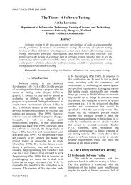
Figure 2(a) and (b) show the diagnosis<br />
performance <strong>of</strong> <strong>HMLP</strong> network versus<br />
different number <strong>of</strong> epochs in the training<br />
and testing phase respectively. During the<br />
analysis, the number <strong>of</strong> hidden nodes is set to<br />
10 hidden nodes. For every epoch in both<br />
phases, the <strong>HMLP</strong> network produced good<br />
diagnosis performance. The performance is<br />
maintained from 1 to 50 epochs. Both figures<br />
indicate that the <strong>HMLP</strong> network achieved its<br />
optimum diagnosis performance after it was<br />
trained for 5 epochs.<br />
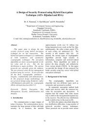
Determination <strong>of</strong> optimum hidden nodes<br />
<strong>of</strong> <strong>HMLP</strong> network is done based on the<br />
results shown in Figure 3(a) and (b). Figure<br />
3(a) and (b) show the diagnosis performance<br />
<strong>of</strong> <strong>HMLP</strong> network during training and<br />
testing phase respectively. During the<br />
analysis, the <strong>HMLP</strong> network was trained for<br />
5 epochs. From both figures, the diagnosis<br />
performance <strong>of</strong> <strong>HMLP</strong> networks are high<br />
and consistent. The <strong>HMLP</strong> network reached<br />
the optimum diagnosis performance after 10<br />
hidden nodes were used.<br />
Analysis percentage<br />
100<br />
80<br />
60<br />
40<br />
20<br />
0<br />
0 10 20 30 40 50<br />
Number <strong>of</strong> epochs<br />
Accuracy<br />
Sensitivity<br />
Specificity<br />
False negative<br />
False positive<br />
Fig 2(a) Training phase<br />
International <strong>Journal</strong> <strong>of</strong> The Computer, The Internet and Management, Vol. 11, No.1, 2003, pp. 17 - 29<br />
23
N. A. Mat-Isa, M. Y. Mashor, N. H. Othman<br />
100<br />
Analysis percentage<br />
80<br />
60<br />
40<br />
20<br />
Accuracy<br />
Sensitivity<br />
Specificity<br />
False negative<br />
False positive<br />
0<br />
0 10 20 30 40 50<br />
Number <strong>of</strong> epochs<br />
(b) Testing phase<br />
Figure 2: Diagnosis performance <strong>of</strong> <strong>HMLP</strong> network for different number <strong>of</strong> epochs.<br />
100<br />
Analysis percentage<br />
80<br />
60<br />
40<br />
20<br />
Accuracy<br />
Sensitivity<br />
Specificity<br />
False negative<br />
False positive<br />
0<br />
0 10 20 30 40 50<br />
Number <strong>of</strong> hidden nodes<br />
(a) Training phase<br />
Analysis percentage<br />
100<br />
80<br />
60<br />
40<br />
20<br />
Accuracy<br />
Sensitivity<br />
Specificity<br />
False negative<br />
False positive<br />
0<br />
0 10 20 30 40 50<br />
Number <strong>of</strong> hidden nodes<br />
(b) Testing phase<br />
Figure 3: Diagnosis performance <strong>of</strong> <strong>HMLP</strong> network for different number <strong>of</strong> hidden nodes.<br />
24
After the <strong>HMLP</strong> network has been<br />
trained using MRPE algorithm, the result in<br />
Figure 2 and 3 show that the <strong>HMLP</strong> network<br />
needed 10 hidden nodes and 5 training<br />
epochs to produce optimum diagnosis<br />
performance. After the <strong>HMLP</strong> network has<br />
been properly trained, the <strong>HMLP</strong> network<br />
was tested using the training and testing data<br />
sets. The overall diagnosis result is shown in<br />
Table 2. The percentage <strong>of</strong> correct<br />
determination <strong>of</strong> normal, LSIL and HSIL<br />
cells are shown in Table 3. The result for<br />
diagnosis confidence level analysis for<br />
determination <strong>of</strong> normal, LSIL and HSIL<br />
cells are shown in Figure 4, 5 and 6<br />
respectively. From these figures, 6 levels <strong>of</strong><br />
diagnosis confidence are used. Level 1 to 5<br />
denotes the proposed diagnosis confidence<br />
level, while Level 6 denote the case <strong>of</strong><br />
incorrect cell determination.<br />
The results in Table 2 indicated that the<br />
<strong>HMLP</strong> network gave good diagnosis<br />
performance. In the training phase, the<br />
<strong>HMLP</strong> network produced 96.09%, 94.79%<br />
and 100% <strong>of</strong> accuracy, sensitivity and<br />
specificity respectively, while in the testing<br />
phase, the <strong>HMLP</strong> network produced 94.44%,<br />
92.59% and 100% <strong>of</strong> accuracy, sensitivity<br />
and specificity respectively. In both phases,<br />
the <strong>HMLP</strong> network produced low percentage<br />
<strong>of</strong> false negative and false negative rate. In<br />
the training phase, only 1.04% <strong>of</strong> false<br />
negative and 6.25% <strong>of</strong> false positive cases<br />
occurred, while in the testing phase, only<br />
5.55% <strong>of</strong> false negative and 2.78% false<br />
positive cases occurred.<br />
Table 2: Overall cervical cancer diagnosis result.<br />
Analysis Training phase Testing phase<br />
Accuracy 96.09 94.44<br />
Sensitivity 94.78 92.59<br />
Specificity 100.00 100.00<br />
False negative 1.04 5.55<br />
False positive 6.25 2.78<br />
Table 3: Percentage <strong>of</strong> correct determination <strong>of</strong> normal, LSIL and HSIL cells.<br />
Type <strong>of</strong> cell Training phase Testing phase<br />
Normal cells 100.00 100.00<br />
LSIL cells 87.50 94.44<br />
HSIL cells 98.44 91.67<br />
Overall 96.09 94.44<br />
The results in Table 3 showed that the<br />
<strong>HMLP</strong> network has superior ability to<br />
determine all normal cells correctly in both<br />
phases. The <strong>HMLP</strong> network also produced<br />
high percentage <strong>of</strong> correct determination for<br />
HSIL cells, which is 98.44% and 91.67% for<br />
training and testing phase respectively. The<br />
percentage <strong>of</strong> correct determination for LSIL<br />
International <strong>Journal</strong> <strong>of</strong> The Computer, The Internet and Management, Vol. 11, No.1, 2003, pp. 17 - 29<br />
25
N. A. Mat-Isa, M. Y. Mashor, N. H. Othman<br />
cells in the testing phase is also high, which<br />
is 94.44%. However, the percentage <strong>of</strong><br />
correct determination for LSIL cells is<br />
slightly low in the training phase, which is<br />
87.50%.<br />
Overall, the results in Table 3 only give<br />
the percentage <strong>of</strong> correct determination for<br />
all type <strong>of</strong> cervical cells without giving a<br />
clear picture on the strength and confidence<br />
level <strong>of</strong> each diagnosis which was done by<br />
<strong>HMLP</strong> network. The strength and confidence<br />
level <strong>of</strong> diagnosis are shown in Figure 4, 5<br />
and 6 for determination <strong>of</strong> normal, LSIL and<br />
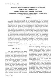
HSIL respectively. From Figure 4, although<br />
the <strong>HMLP</strong> network can determine all normal<br />
cells correctly, but only 81.25% and 72.22%<br />
normal cells are determined with highest<br />
confidence level in training and testing phase<br />
respectively. In training phase, another<br />
15.63% and 3.13% normal cells are<br />
determined correctly with high and moderate<br />
confidence level respectively. While, in the<br />
testing phase 11.11% and 16.67% normal<br />
cells are determined correctly with high and<br />
moderate confidence level respectively.<br />
From Table 3, the <strong>HMLP</strong> network<br />
determined 87.50% and 94.44% LSIL cells<br />
correctly in the training and testing phase<br />
respectively. However, as shown in Figure 5,<br />
in the training phase, it is only about 50%<br />
LSIL cells are determined correctly with<br />
confidence level more than moderate and in<br />
the testing phase the percentage is lower,<br />
which is only about 40%. About 35% and<br />
55% LSIL cells are determined correctly<br />
with low and lowest confidence level in the<br />
training and testing phase respectively.<br />
On the other hand, the <strong>HMLP</strong> network<br />
can determine HSIL cells correctly with<br />
better confidence level as compared to LSIL<br />
cells as shown in Figure 6. In the training<br />
phase, 43.75%, 17.19% and 7.18% HSIL<br />
cells were determined correctly with highest,<br />
high and moderate confidence level<br />
respectively. Only 21.87% and 7.81% HSIL<br />
cells are determined correctly with low and<br />
lowest confidence level respectively. In the<br />
testing phase, 69.44%, 8.33% and 5.56%<br />
HSIL cells are determined correctly with<br />
highest, high and moderate confidence level<br />
respectively. Only 8.33% HSIL cells are<br />
determined correctly with low confidence<br />
level.<br />
Diagnosis Percentage<br />
90<br />
80<br />
70<br />
60<br />
50<br />
40<br />
30<br />
20<br />
10<br />
0<br />
1 2 3 4 5 6<br />
Diagnosis Confidence Level<br />
Training Phase<br />
Testing Phase<br />
Figure 4: Diagnosis confidence level results for determination <strong>of</strong> normal cells.<br />
26
Diagnosis Percentage<br />
100<br />
80<br />
60<br />
40<br />
20<br />
0<br />
1 2 3 4 5 6<br />
Diagnosis Confidence Level<br />
Training phase<br />
Testing phase<br />
Figure 5: Diagnosis confidence level results for determination <strong>of</strong> LSIL cells.<br />
Diagnosis Percentage<br />
100<br />
80<br />
60<br />
40<br />
20<br />
0<br />
1 2 3 4 5 6<br />
Diagnosis Confidence Level<br />
Training phase<br />
Testing phase<br />
Figure 6: Diagnosis confidence level results for determination <strong>of</strong> HSIL cells.<br />
6. Conclusion<br />
The <strong>HMLP</strong> network trained using<br />
MRPE algorithm has been proposed to<br />
classify cervical cells into normal, LSIL and<br />
HSIL cells. Four features from Pap smear<br />
samples, which are size <strong>of</strong> nucleus, size <strong>of</strong><br />
cytoplasm, grey level <strong>of</strong> nucleus and grey<br />
level <strong>of</strong> cytoplasm, have been used as<br />
<strong>HMLP</strong> network inputs data. From the result<br />
in the previous section, it has been proved<br />
that the <strong>HMLP</strong> network has successfully<br />
classified cervical cells with high accuracy,<br />
sensitivity and specificity, and low false<br />
negative and false positive. The <strong>HMLP</strong> has<br />
also successfully determined each type <strong>of</strong><br />
cervical cells correctly with high percentage<br />
in both training and testing phase.<br />
Two new analysis techniques namely<br />
diagnosis confidence percentage and<br />
diagnosis confidence level analysis have<br />
been introduced as diagnosis performance<br />
analysis techniques. Both analyses have been<br />
proved to give significant information about<br />
the strength and confidence level <strong>of</strong> each<br />
diagnosis which is done by <strong>HMLP</strong> network.<br />
From the confidence level analysis, the user<br />
will know either the diagnosis results can be<br />
accepted with or without confirmation by the<br />
International <strong>Journal</strong> <strong>of</strong> The Computer, The Internet and Management, Vol. 11, No.1, 2003, pp. 17 - 29<br />
27
N. A. Mat-Isa, M. Y. Mashor, N. H. Othman<br />
cytopathologist. The high confidence level<br />
indicates that the diagnosis result can be<br />
accepted without any doubt, while the low<br />
confidence level indicates that the diagnosis<br />
result must be confirmed by the pathologist.<br />
References<br />
1. Adami, H. O., Ponten, J., Sparen, P.,<br />
Bergstrom, R., Gustafsson, L. & Friberg,<br />
L. G. (1994). “Survival Trend After<br />
Invasive <strong>Cervical</strong> <strong>Cancer</strong> Diagnosis in<br />
Sweden Before and After Cytologic<br />
Screening”. <strong>Cancer</strong>. Vol. 73. No. 1. pp.<br />
140-147.<br />
2. Balasubramaniam, R., Rajan, S.,<br />
Doraiswami, R. & Stevenson, M. (1998).<br />
“A Reliable Composite <strong>Classification</strong><br />
Strategy”. Proceedings <strong>of</strong> IEEE<br />
Canadian Conference on Electrical and<br />
Computer Engineering. Vol. 2. pp. 914-<br />
917.<br />
3. Breen, N., Wagener, D. K., Brown, M.<br />
L., Davis, W. W. & Barbash, R. B.<br />
(2001). “Progress in <strong>Cancer</strong> Screening<br />
Over a Decade: Results <strong>of</strong> <strong>Cancer</strong><br />
Screening From the 1987, 1992 and 1998<br />
National Health Interview Surveys”.<br />
<strong>Journal</strong> <strong>of</strong> the National <strong>Cancer</strong> Institute.<br />
Vol. 93. No. 22. pp. 1704-1713.<br />
4. Chen, S., Cowan, C. F. N., Billings, S.<br />
A., & Grant, P. M. (1990). “A Parallel<br />
Recursive Prediction Error Algorithm for<br />
Training Layered Neural Networks”.<br />
International <strong>Journal</strong> <strong>of</strong> Control. Vol.<br />
51. No. 6. pp. 1215-1228.<br />
5. Crum, C. P. (1994). Female Genital<br />
Tract. In Robbins: Pathologic Basis <strong>of</strong><br />
Disease. (Cotran, R. S., Kumar, V. &<br />
Robbins, S. L.). pp. 1033-1088. 5 th<br />
Edition. Philadelphia: W. B. Saunders<br />
Company<br />
6. Framer, P. S. (2001). “Screening for<br />
<strong>Cancer</strong>: Progress but More Can Be<br />
Done”. <strong>Journal</strong> <strong>of</strong> the National <strong>Cancer</strong><br />
Institute. Vol. 93. No. 22. pp. 1676-1677.<br />
7. Hislop, T. G., Band, P. R., Deschamps,<br />
M., Clarke, H. F., Smith, J. M. & Ng, V.<br />
T. Y. (1994). “<strong>Cervical</strong> <strong>Cancer</strong> Screening<br />
in Canadian Native Women: Adequacy<br />
<strong>of</strong> The Papnicolaou Smear”. The <strong>Journal</strong><br />
<strong>of</strong> Clinical Cytology and Cytopathology.<br />
Vol. 38. No. 1. pp. 29-32.<br />
8. HTAC. (2002). “Pap Smears and<br />
Prevention <strong>of</strong> <strong>Cervical</strong> <strong>Cancer</strong>”. Citing<br />
from internet source URL<br />
http://www.health.state.mn.us/htac/papq<br />
&a.html.<br />
9. Kuie, T. S. (1996). <strong>Cervical</strong> <strong>Cancer</strong>: Its<br />
Causes and Prevention. Singapore:<br />
Times Book International.<br />
10. Li, Z. & Najarian, K. (2001).<br />
“Automated <strong>Classification</strong> <strong>of</strong> Pap Smear<br />
Tests <strong>Using</strong> Neural Networks”.<br />
Proceedings <strong>of</strong> International Joint<br />
Conference on Neural Networks. Vol. 4.<br />
pp. 2899-2901.<br />
11. Mashor, M. Y. (2000). “Hybrid<br />
Multilayered Perceptron Networks”.<br />
International <strong>Journal</strong> <strong>of</strong> System Science.<br />
Vol. 31. No. 6. pp. 771-785.<br />
12. Mat-Isa, N. A., Mashor, M. Y. &<br />
Othman, N. H. (2001). “Diagnosis <strong>of</strong><br />
<strong>Cervical</strong> <strong>Cancer</strong> <strong>Using</strong> Hybrid Radial<br />
Basis Function Network’. Proceedings <strong>of</strong><br />
Student Conference on Research and<br />
Development. pp. 37.<br />
13. Mat-Isa, N. A., Mashor, M. Y. &<br />
Othman, N. H. (2002). “Diagnosis <strong>of</strong><br />
<strong>Cervical</strong> <strong>Cancer</strong> <strong>Using</strong> Hierarchical<br />
28
Radial Basis Function (HiRBF)<br />
Network’. Proceedings <strong>of</strong> International<br />
Conference on Artificial Intelligence in<br />
Engineering and Technology. pp. 458-<br />
463.<br />
14. Ministry <strong>of</strong> Health Malaysia. (1999).<br />
Malaysia’s Health 1999: Technical<br />
Report <strong>of</strong> The Director-General <strong>of</strong><br />
Health, Malaysia 1999. Malaysia:<br />
Ministry <strong>of</strong> Health Malaysia.<br />
15. Mitra, P., Mitra, S. & Pal, S. K. (2000).<br />
“Staging <strong>of</strong> <strong>Cervical</strong> <strong>Cancer</strong> with S<strong>of</strong>t<br />
Computing”. IEEE Transaction on<br />
Biomedical Engineering. Vol. 47. No. 7.<br />
934-940.<br />
16. Othman, N. H., Ayub, M. C., Aziz, W.<br />
A. A., Muda, M., Wahid, R. &<br />
Selvarajan, S. (1997). “Pap Smears – Is It<br />
An Effective Screening Methods for<br />
<strong>Cervical</strong> <strong>Cancer</strong> Neoplasia? – An<br />
Experience with 2289 Cases”. The<br />
Malaysian <strong>Journal</strong> <strong>of</strong> Medical Sciences.<br />
Vol. 4. No. 1. pp. 45-50.<br />
17. Othman, N. H., Ayob, M. C. & Wahid,<br />
R. A. (1995). “Is Pap Smear Screening<br />
Program Effective? A Kelantan<br />
Experience with 5000 cases”. Malaysian<br />
<strong>Journal</strong> <strong>of</strong> Pathology. Vol. 17. No. 1. pp.<br />
53.<br />
18. WebMD. (2002). “How Can <strong>Cervical</strong><br />
<strong>Cancer</strong> Be Prevented?”. Citing from<br />
internet source URL<br />
http://www.webmd.com/content/dmk/dmk<br />
_article_3961643.<br />
***<br />
International <strong>Journal</strong> <strong>of</strong> The Computer, The Internet and Management, Vol. 11, No.1, 2003, pp. 17 - 29<br />
29