A Brief Introduction to Space Plasma Physics.pdf - Institute of ...

ESS 200C - Space Plasma Physics
Winter Quarter 2006-2007
Date Topic
1/8 Organization and Introduction
to Space Physics I
1/10 Introduction to Space Physics II
1/17 Introduction to Space Physics III
1/19 The Sun I
1/22 The Sun II
1/24 The Solar Wind I
1/29 The Solar Wind II
1/31 First Exam
2/5 Bow Shock and Magnetosheath
2/7 The Magnetosphere I
Raymond J. Walker
Schedule of Classes
Date Topic
2/14 The Magnetosphere II
2/16 The Magnetosphere III
2/21 Planetary Magnetospheres
2/23 The Earth’s Ionosphere
2/26 Substorms
3/5 Aurorae
3/7 Planetary Ionospheres
3/12 Pulsations
3./14 Storms and Review
Second Exam

ESS 200C – Space Plasma
Physics
• There will be two examinations and homework assignments.
• The grade will be based on
– 35% Exam 1
– 35% Exam 2
– 30% Homework
• References
– Kivelson M. G. and C. T. Russell, Introduction to Space
Physics, Cambridge University Press, 1995.
– Gombosi, T. I., Physics of the Space Environment, Cambridge
University Press, 1998
– Kellenrode, M-B, Space Physics, An Introduction to Plasmas and
Particles in the Heliosphere and Magnetospheres, Springer, 2000.
– Walker, A. D. M., Magnetohydrodynamic Waves in Space, Institute
of Physics Publishing, 2005.

Space Plasma Physics
• Space physics is concerned with the interaction of
charged particles with electric and magnetic fields in
space.
• Space physics involves the interaction between the
Sun, the solar wind, the magnetosphere and the
ionosphere.
• Space physics started with observations of the
aurorae.
– Old Testament references to auroras.
– Greek literature speaks of “moving accumulations
of burning clouds”
– Chinese literature has references to auroras prior
to 2000BC

• Aurora over Los Angeles (courtesy V.
Peroomian)

– Galileo theorized that aurora is caused by air rising out of
the Earth’s shadow to where it could be illuminated by
sunlight. (Note he also coined the name aurora borealis
meaning “northern dawn”.)
– Descartes thought they are reflections from ice crystals.
– Halley suggested that auroral phenomena are ordered by
the Earth’s magnetic field.
– In 1731 the French philosopher de Mairan suggested they
are connected to the solar atmosphere.

• By the 11th century the
Chinese had learned that
a magnetic needle points
north-south.
• By the 12th century the
European records
mention the compass.
• That there was a
difference between
magnetic north and the
direction of the compass
needle (declination) was
known by the 16th
century.
• William Gilbert (1600)
realized that the field was
dipolar.
• In 1698 Edmund Halley
organized the first
scientific expedition to
map the field in the
Atlantic Ocean.

The Plasma State
• A plasma is an electrically neutral ionized
gas.
– The Sun is a plasma
– The space between the Sun and the Earth
is “filled” with a plasma.
– The Earth is surrounded by a plasma.
– A stroke of lightning forms a plasma
– Over 99% of the Universe is a plasma.
• Although neutral a plasma is composed of
charged particles- electric and magnetic
forces are critical for understanding plasmas.

The Motion of Charged Particles
• Equation of motion
m
r
dv
dt
r
= qE
r r
+ qv × B +
• SI Units
– mass (m) - kg
– length (l) - m
– time (t) - s
– electric field (E) - V/m
– magnetic field (B) - T
– velocity (v) - m/s
– F g stands for non-electromagnetic forces (e.g. gravity) -
usually ignorable.
r
F g

• B acts to change the motion of a charged particle
only in directions perpendicular to the motion.
– Set E = 0, assume B along z-direction.
mv&
mv&
v&&
x
v&&
y
x
y
=
qv
y
= −qv
2
qv&
yB
q vxB
= = −
2
m m
2 2
q vyB
= −
2
m
– Equations of circular motion with angular frequency
(cyclotron frequency or gyro frequency
Ω = qB
c
m
– If q is positive particle gyrates in left handed sense
– If q is negative particle gyrates in a right handed sense
B
x
B
2

• Radius of circle ( r c ) - cyclotron radius or Larmor
radius or gyro radius. v = ρ Ω
mv
qB
– The gyro radius is a function of energy.
– Energy of charged particles is usually given in electron volts
(eV)
– Energy that a particle with the charge of an electron gets in
falling through a potential drop of 1 Volt- 1 eV = 1.6X10 -19
Joules (J).
• Energies in space plasmas go from electron Volts to
kiloelectron Volts (1 keV = 10 3 eV) to millions of electron Volts
(1 meV = 10 6 eV)
• Cosmic ray energies go to gigaelectron Volts ( 1 geV = 10 9 eV).
• The circular motion does no work on a particle
r r
F ⋅v
=
r
dv
m
dt
r
⋅v
⊥
ρ
c
=
c
1
d(
2
mv
=
dt
2
⊥
)
c
r r r
= qv ⋅(
v × B)
= 0
Only the electric field can energize particles!

• The electric field can modify the particles motion.
– Assume E r ≠ 0 but B r still uniform and F g =0.
– Frequently in space physics it is ok to set E
r
⋅ B r
= 0
• Only E r
can accelerate particles along B r
• Positive particles go along E and negative particles go
along − E
• Eventually charge separation wipes out E
E ⊥
– has a major effect on motion.
• As a particle gyrates it moves along E r and gains energy
• Later in the circle it losses energy.
• This causes different parts of the “circle” to have different radii -
it doesn’t close on itself.
r r
r E × B
=
u E
2
B
• Drift velocity is perpendicular to and
• No charge dependence, therefore no currents
E r
B r

• Any force capable of accelerating and decelerating
charged particles can cause
r r
them to drift.
r F × B
u F
=
2
qB
– If the force is charge independent the drift motion will
depend on the sign of the charge and can form
perpendicular currents.
• Changing magnetic fields cause a drift velocity.
– If B r changes over a gyro-orbit the radius of curvature will
change.
mv⊥
– ρc
= gets smaller when the particle goes into a region of
qB
stronger B. Thus the drift is opposite to that of E
r B
r
r r × motion.
r
−1
2 ∇B
× B
1 2 B × ∇B
u g
=
2
mv⊥
=
3 2
mv⊥
3
qB
qB
– u g depends on the charge so it can yield perpendicular
currents.

• The change in the direction of the magnetic field
along a field line can cause motion.
– The curvature of the magnetic field line introduces a drift
motion.
• As particles move along the field they undergo centrifugal
acceleration.
2
r
F
mv
R
nˆ
• R c
is the radius of curvature of a field line ( = −(
bˆ
⋅∇)
bˆ
)
where
Rc
r
B
bˆ = , nˆ is perpendicular to B r
and points away from the center
B
of curvature, v is the component of velocity along B r
r
u
c
=
mv
• Curvature drift can cause currents.
=
c
Rˆ
c
r
B×
( bˆ
⋅∇)
bˆ
2 2
ˆ
qB
2
r
mv B×
n
= −
2
R qB
c

• The Concept of the Guiding Center
v r
– Separates the motion ( ) of a particle into motion
perpendicular ( ) and parallel ( v ) to the magnetic field.
v
⊥
– To a good approximation the perpendicular motion can
consist of a drift ( ) and the gyro-motion ( )
r
v
=
r
v
v D
– Over long times the gyro-motion is averaged out and the
particle motion can be described by the guiding center
motion consisting of the parallel motion and drift. This is very
useful for distances l such that ρ c
l

• Maxwell’s equations
– Poisson’s Equation
∇ ⋅ E r
=
ρ
ε 0
• E r is the electric field
• ρ is the charge density
• ε is the electric permittivity (8.85 X 10 -12 0
Farad/m)
– Gauss’ Law (absence of magnetic monopoles)
∇ ⋅ B r
= 0
• is the magnetic field
B r

– Faraday’s Law
– Ampere’s Law
r
∇× B =
• c is the speed of light.
• Is the permeability of free space, H/m
0
• is the current density
r
r ∂B
∇× E = −
∂t
1
c
2
r
∂E
∂t
r
+ µ J
−7
µ µ = 4π ×
J r
0
0
10

• Maxwell’s equations in integral form
r 1
∫ E ⋅ ndA ˆ = ∫ ρ dV
A
ε 0
– A is the area, dA is the differential element of area
– nˆ is a unit normal vector to dA pointing outward.
– V is the volume, dV is the differential volume element
ˆn '
∫
∫
A
C
r
B ⋅ nd ˆ A =
v r
E ⋅ ds = −
0
r
∂B
∂t
'
⋅nˆ
dF = −
∂Φ
∂ t
– is a unit normal vector to the surface element dF in the
direction given by the right hand rule for integration around
C, and is magnetic flux through the surface.
ds
r
Φ
– is the differential element
r
around C.
r r ∂E
'
∫ B ⋅ds
= 2 n dF J
C
c ∫ ⋅ ˆ + µ
0
∂t
∫
∫
1
ˆ
'
⋅n dF

• The first adiabatic invariant
r
∂B
r
– = −∇× E says that changing B r
drives E r
(electromotive
∂t
force). This means that the particles change energy in
changing magnetic fields.
– Even if the energy changes there is a quantity that remains
constant provided the magnetic field changes slowly enough.
– µ is called the magnetic moment. In a wire loop the
magnetic moment is the current through the loop times the
area.
µ
1 2
2
mv =
⊥ =
B
– As a particle moves to a region of stronger (weaker) B it is
accelerated (decelerated).
const.

• For a coordinate in which the motion is
periodic the action integral
J
i
= ∫ pidqi
= constant
is conserved.
rHere pr
i is the rcanonical
momentum ( p = mv + qA where A is the
vector potential).
r r 2πm
• For a gyrating particle J1 = ∫ p⊥
⋅ds
= µ
q
• The action integrals are conserved when the
properties of the system change slowly
compared to the period of the coordinate.

• The magnetic mirror
– As a particle gyrates the current will be
I =
q
T c
where
T c
= π
Ω
c
– The force on a dipole magnetic moment is
where
A = π r
IA
=
π v
2
c
2
⊥
2π
Ω
v
= π
Ω
q Ω
c
2
c
=
2
⊥
2
c
mv
2B
r
dB
F = −
r µ ⋅∇B
= −µ
r
dz
µ = µ bˆ
2
⊥
=
2 µ

B r
• The force is along and away from the direction of
increasing B.
• Since E = 0 and kinetic energy must be conserved
1 2 1 2 2
2
mv =
2
m(
v + v⊥)
a decrease in v must yield an increase in v⊥
• Particles will turn around when
B =
1
mv
2
2
µ

• The second adiabatic invariant
– The integral of the parallel momentum over one
complete bounce between mirrors is constant (as
long as B doesn’t change much in a bounce).
J
= ∫
s
s
1
2
2mv
ds
= const.
– Using conservation of energy and the first
adiabatic invariant
J
= ∫
s
s
1
2
B
2
2mv(1
− )
1
ds
B
here B m is the magnetic field at the mirror point.
m
= const.

– As particles bounce they will drift
because of gradient and
curvature drift motion.
– If the field is a dipole their
trajectories will take them around
the planet and close on
themselves.
• The third adiabatic invariant
– As long as the magnetic field
doesn’t change much in the time
required to drift around a rplanet
the magnetic flux Φ = ∫ B ⋅ nˆ
dA
inside the orbit must be constant.
– Note it is the total flux that is
conserved including the flux
within the planet.

• Limitations on the invariants
µ
– is constant when there is little change in the field’s
strength over a cyclotron path.
∇B
B
– All invariants require that the magnetic field not change much in the
time required for one cycle of motion
1
B

The Properties of a Plasma
• A plasma as a collection of particles
– The properties of a collection of particles can be described
by specifying how many there are in a 6 dimensional volume
called phase space.
• There are 3 dimensions in “real” or configuration space and 3
dimensions in velocity space.
• The volume in phase space is
dvdr
• The number of particles in a phase space volume is
where f is called the distribution function.
– The density of particles of species “s” (number per unit
volume)
– The average velocity (bulk flow velocity)
r
u
s
r
(
, t)
=
dv
r r r
ns (
, t)
= ∫ fs
(
, v,
t)
dv
x
dv
y
dv
z
dxdydz
r r r r r
= vf (
, v,
t)
dv / f (
, v,
t)
dv
∫
s
∫ s
r r
f (
, v,
t)
dvdr

– Average random energy
r r 2
− = ∫
2 r r r
1
ms ( v us
) ms
( v − us
) fs
(
, v,
t)
dv / fs
(
, v,
t)
dv
r
1
2
2
– The partial pressure of s is given by
p
n
s
s
2
N
=
( ) 2 3r −
1 2
(
2ms
( v us
)
where N is the number of independent velocity components
(usually 3).
r
∫
– In equilibrium the phase space distribution is a Maxwellian
distribution
r r
⎡ 1
2
r r
( )
( − ) ⎤
2
ms
v us
fs
, v = As
exp⎢
⎥⎦
⎣ kTs
where
A
s
= n
s
m
2π
kT

• For monatomic particles in equilibrium
1 2
2m
( ) NkT
s
v us
= / 2
p
s
=nskTs
where k is the Boltzman constant (k=1.38x10 -23 JK -1 )
• For monatomic particles in equilibrium
m v
r − u
r 2
= NkT
1
2
( ( ) ) 2
• This is true even for magnetized particles.
• The ideal gas law becomes
s
r
− r
s
p = n
s
s
kT
s
s

– Other frequently used distribution functions.
• The bi-Maxwellian distribution
⎡ 1
r r
ms
v − u
'
2
f ( ) = ⎢
s
, v As
exp −
⎢ kT
⎣
s
– where
s s s ⎜ s s ⎟
⎝ ⎠
– It is useful when there is a difference between the distributions
perpendicular and parallel to the magnetic field
• The kappa distribution
f
s
r
'
A
r
( r,
v)
=
A
Κ characterizes the departure from Maxwellian form.
– E Ts is an energy.
κs
⎡
⎢1
+
⎣
2
( ) ⎤ r r
⎡ 1
2
( ) ⎤
⎥⎦
1
2
m
s
⎥ exp⎢−
⎥
⎦ ⎣
( v − u )
sκ Ts
s
− u
– At high energies E>>κE Ts it falls off more slowly than a Maxwellian
(similar to a power law)
κ → ∞
⎛
⎜T
3
2
= A T
⊥
T
1
2
⎞
⎟
– For it becomes a Maxwellian with temperature kT=E Ts
r
E
r
2
2
⎤
⎥
⎦
m
s
v
−κ
−1
⊥
kT
⊥s
⊥s

• What makes an ionized gas a plasma?
– The electrostatic potential of an isolated ion ϕ =
q
4πε 0
r
– The electrons in the gas will be attracted to the ion and will reduce
the potential at large distances.
– If we assume neutrality Poisson’s equation around a test charge
q 0
is
∇
– Expanding in a Taylor series for r>0 and for both
–
ϕ
r − ρ q
⎡ ⎛ ⎞ ⎛ ⎞⎤
0 3 en0
eϕ
− eϕ
( ) = = − δ ( r ) + exp⎜
⎟ − exp⎜
⎟⎥ ⎦
2 r
ε
0
electrons and ions
∇
ϕ
r
2
ε
0
en ⎡
⎢
ε
0 ⎣
eϕ
kT
ε
0
⎢
⎣
eϕ
⎤
⎥
kTion
⎦
⎜
⎝ kT
⎟
⎠
eϕ kT
⎜
⎝
e
kT ion

ϕ =
−r
λ
qe D
4π
ε 0
r
•The Debye length ( ) is
where n is the electron number density and now e
is the electron charge.
•The number of particles within a Debye sphere
N
D
3
4π
nλ
=
D
3
λ
needs to be large for shielding to occur
(N D >>1). Far from the central charge the electrostatic
force is shielded.
D
λ D
⎛ 0kT
= ⎜ ne
2
⎝
ε
⎞
⎟
⎠
1
2

• The plasma frequency
– Consider a slab of plasma of thickness L.
– At t=0 displace the electron part of the slab by

– The frequency of this oscillation is the plasma frequency
ω
ω
ω
2
p
2
pe
0 ion
– Because m ion >>m e
ω ≈
2
pi
= ω
2
pe
2
e n0
=
ε
0m
2
e n
=
ε m
+ ω
e
0
p
ω pe
2
pi

• A note on conservation laws
– Consider a quantity that can be moved from place to place.
f r
– Let be the flux of this quantity – i.e. if we have an element of area
then is the amount of the quantity passing the area
element per unit time.
– Consider a volume V of space, bounded by a surface S.
– If σ is the density of the substance then the total amount in the
volume is
r r
f ⋅δ
A
∫σ dV
– The rate at which material is lost through the surface is
d
r r
∫σ
dV = −∫ f ⋅ dA
dt
– Use Gauss’ theorem
V
– An equation of the preceeding form means that the quantity whose
density is σ is conserved.
∫
V
V
⎧∂σ
⎨ + ∇ ⋅
⎩ ∂t
∂σ
= −∇ ⋅
∂t
S
r⎫
f ⎬dV
⎭
r
f
= 0
r r
∫ f ⋅dA
S
δA r

• Magnetohydrodynamics (MHD)
– The average properties are governed by the basic
conservation laws for mass, momentum and energy in a
fluid.
– Continuity equation
∂n
∂t
s
+ ∇ ⋅ n
– S s and L s represent sources and losses. S s -L s is the net rate
at which particles are added or lost per unit volume.
– The number of particles changes only if there are sources
and losses.
s
r
u
– S s ,L s ,n s , and u s can be functions of time and position.
– Assume S s =0 and L s =0, ρ s= m
sn
, s ∫ ρ sdr
= M
s where M s is
the total mass of s and dr is a volume element (e.g. dxdydz)
∂M
s
r ∂M
s
r r
+ ∇ ⋅
sus
dr = +
sus
⋅ds
∂t
∫ (ρ )
∂t
∫ ρ
where ds
r is a surface element bounding the volume.
s
=
S
s
−
L
s

– Momentum equation
r
∂us
r r r
r r r
ρ
s
( + us
⋅∇us
) + msus
( Ss
− Ls
) = −∇ps
+ ρqsE
+ J
s
× B + ρsF
∂t
ρ
= q
n
r
J =
where qs s s is the charge density, s s s s is the
current density, and the last term is the density of nonelectromagnetic
forces
∂ r
– The operator ( + u s
⋅∇)
is called the convective derivative
∂t
and gives the total time derivative resulting from intrinsic
time changes and spatial motion.
– If the fluid is not moving (u s =0) the left side gives the net
change in the momentum density of the fluid element.
– The right side is the density of forces
• If there is a pressure gradient then the fluid moves toward lower
pressure.
• The second and third terms are the electric and magnetic
forces.
q
n
r
u
g
m
s

u s ⋅∇ u s
0
– The term means that the fluid transports
momentum with it.
• Combine the species for the continuity and
momentum equations
– Drop the sources and losses, multiply the continuity
equations by m s , assume n p =n e and add.
Continuity
∂ρ
r
+ ∇ ⋅( ρ u)
=
∂t
– Add the momentum equations and use m e

• Energy equation
∂
(
∂t
1
2
2
r r r
1 2
ρ u + U)
+∇⋅[(
2
ρu
+ U)
u + pu + q]
=
q r
where is the heat flux, U is the internal energy
density of the monatomic plasma ( U = nNkT / 2) and
N is the number of degrees of freedom
q r
treated by making approximations so it can be handled by
the other variables.
the fluid element)
−γ
∂p
r ∂ρ
r
p = const.
+ u ⋅∇p
= c
2
s
( + u ⋅∇ρ
– adds three unknowns to our set of equations. It is usually
– Make the adiabatic assumption (no change in the entropy of
ρ or
)
∂t
∂t
2
where c s is the speed of sound c s
= γ p ρ and γ = c p
c v
c p and c v are the specific heats at constant pressure and
constant volume. It is called the polytropic index. In
thermodynamic equilibrium γ = ( N + 2) N = 5 / 3
r r r r
J ⋅E
+ ρu
⋅F
g
m

• Maxwell’s equations
r
∂B
r
= −∇× E
∂t
r r
∇× B = µ 0
J
– ∇ ⋅ B r = 0 doesn’t help rbecause
∂(
∇ ⋅ B)
r
= −∇ ⋅∇× E = 0
∂t
r r r
– There are 14 unknowns in this set of equations - r
E , B,
J , u,
ρ,
p
– We have 11 equations.
• Ohm’s law
– Multiply the momentum equations for each individual species
by q s /m s and subtract
r
J
r
r r r 1 1 r r me
∂J
rr
= σ {( E + u × B)
+ ∇pe
− J × B − [ + ∇ ⋅(
Ju)]}
2
ne ne ne ∂t
r r
where J = ∑ qsnsusand σ is the electrical conductivity
s

– Often the last terms on the right in Ohm’s Law can be dropped
– If the plasma is collisionless, may be very large so
• Frozen in flux
r r r r
J = σ ( E + u × B)
σ
r r r
E + u × B = 0
– Combining Faraday’s law ( ), and
r
∇× B
Ampere’ law ( ) with
r
∂B
∂t
η
m
= 1 σ µ 0
r
r ∂B
∇× E = −
r r ∂rt
r r
= µ 0
J J = σ ( E + u × B)
r r r
2
= ∇× ( u × B)
+ η ∇ B
where is the magnetic viscosity
– If the fluid is at rest this rbecomes a “diffusion” equation
∂B
r
2
= ηm∇
B
∂t
– The magnetic field will exponentially decay (or diffuse) from a
2
conducting medium in a time τ D
= L η where L B
is the system size.
m
B
m

– On time scales much shorter than
r
∂B
∂t
r r
= ∇× ( u × B)
– The electric field vanishes in the frame moving with the fluid.
– Consider the rate of change of magnetic flux
dΦ
dt
=
d
dt
r
∂B
∂t
∫ B ⋅ndA
= ∫ ⋅ ndA + ∫ B ⋅(
u ×
A
r
ˆ
– The first term on the right is caused by the temporal changes
in B
– The second term is caused by motion of the boundary
– The term is the area swept out per unit time
A
r r
u × dl
0
– Use Stoke’s theorem
Φ r
d ⎛ ∂
⎞
= ∫ B r r
⎜ ( ) ⎟
− ∇× u × B
⋅ nˆ
=
dt ⎝ ∂
dA
A
t
⎠
– If the fluid is initially on surface s as it moves through the
system the flux through the surface will remain constant
even though the location and shape of the surface change.
ˆ
τ D
C
r
r
r
dl )

F B
• Magnetic pressure and tension
=
r
J ×
r
B
=
1 2
)
µ
( ∇× B)
× B = −∇B
2µ
0
+ ( B ⋅∇ B
0
r
r
r
r
µ
0
2
– p B
= B
A magnetic pressure analogous to the plasma
2µ
pressure ( )
β ≡
B
p
– 2 A “cold” plasma has β

2
– bˆ
B ⋅∇B
ˆ ˆ∇B
cancels the parallel component
2
− ∇B 2µ
0
component of the magnetic pressure exerts a force on the
of the term. Thus only the perpendicular
plasma.
= bb
µ
0
2
µ
0
2
2
ˆ
– ( B ˆ ˆ nB
) b ⋅∇b
= −(
) is the magnetic tension
µ
0 µ
0R C
and is directed antiparallel to the radius of
curvature (R C ) of the field line. Note that nˆ is
directed outward.

•Some elementary wave concepts
–For a plane wave propagating in the x-direction with
wavelength λ and frequency f, the oscillating quantities
can be taken to be proportional to sines and cosines.
For example the pressure in a sound wave propagating
along an organ pipe might vary like
p
=
p0 sin( kx −ωt)
–A sinusoidal wave can be described by its frequency
k r
r r r r
r r
B( r,
t)
= B0 cos(
r
k ⋅
−ωt
v
) + i sin( k ⋅
−ωt)
r
B( r,
t)
= B0 exp{ i(
k ⋅
−ωt)}
and wave vector . (In the organ pipe the frequency is
f and ω = 2π f . The wave number is k = 2π λ ).
r
( )
ω

• The exponent gives the phase of the wave.
The phase velocity specifies how fast a feature
of a monotonic wave is moving
v ph
=
ω r
k
2
k
•Information propagates at the group velocity. A
wave can carry information provided it is formed
from a finite range of frequencies or wave
numbers. The group velocity is given by
∂
v g
= r
ω
∂k
•The phase and group velocities are calculated
and waves are analyzed by determining the
dispersion relation
ω = ω(k)

• When the dispersion relation shows asymptotic
behavior toward a given frequency, ω res
, v g goes to
zero, the wave no longer propagates and all the wave
energy goes into stationary oscillations. This is called a
resonance.

• MHD waves - natural wave modes of a
magnetized fluid
– Sound waves in a fluid
• Longitudinal compressional oscillations which propagate
at
c s
=
⎛
⎜
⎝
∂
∂
p ⎞
⎟
ρ ⎠
1
2
⎛ γ p
= ⎜
⎝ ρ
1
2
⎞
⎟
⎠
1
2
⎡
• ⎛ kT ⎞⎤
c s
= ⎢γ
⎜ ⎟⎥and is comparable to the thermal speed.
⎣ ⎝ m ⎠⎦

– Incompressible Alfvén waves
• Assume σ → ∞ , incompressible fluid with B r background
0
field and homogeneous
z
B 0
J
b, u
y
• Incompressibility
x
∇ ⋅u r = 0
• We want plane wave solutions b=b(z,t), u=u(z,t), b z
=u z
=0
• Ampere’s law gives the current
r
1
∂ b
J = − iˆ
µ 0
∂ z
u r ⋅∇
• Ignore convection ( )=0
r
∂u
ρ = −∇p
+
∂t
r r
J × B

∂p
∂x
• Since = 0 , = 0 and = 0 the x-component of
momentum becomes
• Faraday’s law gives
• The y-component of the momentum equation
becomes
J y
J z
∂ux
∂p
ρ = −
∂t
∂x
r
u = uj ˆ
r
E = −uB iˆ
∂
u y
∂t
0
∂b
∂t
+ ( J
∂E
= −
∂z
• Differentiating Faraday’s law and substituting the y-
component of momentum
2
∂ b
=
2
∂t
x
y
1 r r
= − J × B
B
0
B
=
0
=
− b
B
0
0
ρ
0
2
∂ u
∂z∂t
y
J
∂u
∂z
z
B0
∂b
µ ρ ∂z
2 2
⎛ B ⎞ ∂ b
=
⎜
⎟
2
⎝ µ
0
ρ ⎠ ∂z
) = 0

1
2
2
C ⎛ B ⎞
A ⎜ ⎟
⎝ µ
0
ρ ⎠
• The most general solution is b = b( z ± C t ) . This is a
where = ⎜ ⎟ is called the Alfvén velocity.
disturbance propagating along magnetic field lines at the
Alfvén velocity.
2
∂ b
2
∂t
=
C
∂
u
2
2
A 2
∂z
A

• Compressible solutions
– In general incompressibility will not always apply.
– Usually this is approached by assuming that the system
starts in equilibrium and that perturbations are small.
• Assume uniform B 0
, perfect conductivity with equilibrium
pressure p 0
and mass density ρ 0
ρ = ρ 0
+ ρ
p
r
B
r
u
r
J
r
E
T
T
T
T
T
T
= p
r
= B
r
= u
r
= J
r
= E
0
0
+ p
r
+ b

– Continuity
– Momentum
– Equation of state ∇p
=
– Differentiate the momentum equation in time, use Faraday’s
law and the ideal MHD condition
where
∂ρ
r
= −ρ0(
∇ ⋅u)
∂t
r
∂u
1 r r
ρ0 = −∇p
− ( B0
× ( ∇× b))
∂t
µ
0
∂p
( ) 0
∇ρ
= Cs
∂ρ
2
∇ρ
r r r
E = −u
× B0
r
∂b
r r r
= −(
∇× E)
= ∇× ( u × B0
)
∂t
2 r
∂ u 2 r r
r r
− C ∇(
∇ ⋅ ) + × ( ∇× ( ∇× ( ∇× ( ×
2 s
u CA
u C
∂t
r r
=
C A
B
1
0 ) 2
( µ ρ
A
))) = 0

– For a plane wave solution
– The dispersion relationship between the frequency ( ) and
the propagation vector ( ) becomes
This came from replacing derivatives in time and space by
– Case 1
r
r
r
r
r
u
r
~ exp[ i(
k
r ⋅ −ω
t)]
ω
k r r r r r r r r r r r
k )[( C ⋅ k ) u − ( C ⋅u)
k − ( k ⋅u
C ] = 0
2 2 2
− ω u + ( Cs
+ CA)(
k ⋅u)
k + ( CA
⋅
A
A
)
A
k
r ⊥
r
B 0
2 r
ω u
∂
→ −iω
∂t
r
∇ → ik
r
∇⋅ → ik ⋅
r
∇× → ik ×
= ( C
2
s
+
C
2
A
r r r
)( k ⋅u)
k

• The fluid velocity must be along k r and perpendicular to
0
B r
0
k r u r
• These are magnetosonic waves
– Case 2
( k
B r r
1
2
2
v
ph
= k ( ω ) = ± ( C
s+
C
k
k r B r
0
2 2 2 r
r
2 2 2 r r
CA
−ω
) u + (( Cs
CA)
−1)
k ( CA
⋅u)
CA
= 0
r
• A longitudinal mode with u k
r
with dispersion relationship ω
k
(sound waves) r
• A transverse mode with k ⋅u
r
ω
= 0 and = ± C A
(Alfvén
waves)
k
2
A
)
= ±
C s

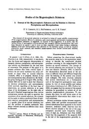
• Alfven waves
propagate parallel to
the magnetic field.
•The tension force acts
as the restoring force.
•The fluctuating
quantities are the
electromagnetic field
and the current density.

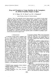
– Arbitrary angle between k r and B r
0
V A =2C S
B r
0
V A
S
I
F
Phase Velocities