Prediction of Flashover Voltage of Insulators Using Low Voltage ...

PSERC
Prediction of Flashover Voltage
of Insulators Using Low Voltage
Surface Resistance Measurement
Final Project Report
Power Systems Engineering Research Center
A National Science Foundation
Industry/University Cooperative Research Center
since 1996

Power Systems Engineering Research Center
Prediction of Flashover Voltage of Insulators Using
Low Voltage Surface Resistance Measurement
Final Project Report
Project Team
Ravi S. Gorur, Project Leader, Arizona State University
Robert Olsen, Washington State University
Industry Advisors
Jim Crane and Tom Adams, Exelon
Jim Gurney and Jim Duxbury,
British Columbia Transmission Corp.
Graduate Student
Sreeram Venkataraman, Arizona State University
PSERC Publication 06-42
November 2006

Information about this project
For information about this project contact:
Ravi S. Gorur, Ph.D.
Professor of Electrical Engineering
Arizona State University
Tempe, AZ 85287-5706
Phone: 480-965-4894
Fax: 480-965-0745
Email: ravi.gorur@asu.edu
Power Systems Engineering Research Center
This is a project report from the Power Systems Engineering Research Center (PSERC). PSERC
is a multi-university Center conducting research on challenges facing a restructuring electric
power industry and educating the next generation of power engineers. More information about
PSERC can be found at the Center’s website: http://www.pserc.org.
For additional information, contact:
Power Systems Engineering Research Center
Arizona State University
577 Engineering Research Center
Box 878606
Tempe, AZ 85287-8606
Phone: 480-965-1643
FAX: 480-965-0745
Notice Concerning Copyright Material
PSERC members are given permission to copy without fee all or part of this publication for
internal use if appropriate attribution is given to this document as the source material. This report
is available for downloading from the PSERC website.
© 2006 Arizona State University. All rights reserved.

ACKNOWLEDGEMENTS
This is the final report for the Power Systems Engineering Research Center (PSERC)
research project titled “Prediction of Flashover Voltage of Insulators Using Low Voltage Surface
Resistance Measurement” (PSERC T-26G). We express our appreciation for the support
provided by PSERC’s industrial members and by the National Science Foundation under grant
NSF EEC-0001880 received from the Industry / University Cooperative Research Center
program.
We also express our appreciation for the special financial support provided by PSERC’s
industrial members, Exelon and British Columbia Transmission Corp (BCTC). Technical
guidance from Mr. Jim Crane and Mr. Tom Adams, Exelon; and Mr. Jim Gurney and Mr. Jim
Duxbury of BCTC is appreciated.
i

EXECUTIVE SUMMARY
Failures of high voltage insulators on transmission lines can lead to transmission line
outages, thereby reducing system reliability. One form of insulator failure is flashover, the
unintended disruptive electric discharge over or around the insulator. Contamination on the
surface of the insulators, such as from salts for de-icing streets and sidewalks, enhances the
chances of flashover. Currently there are no standardized tests for understanding the
contamination flashover performance of polymeric insulators. This research project developed
models by which the flashover voltage can be predicted and flashover dynamics explained for
contaminated polymeric insulators. The model developed can be applied to contaminates such as
sea salt, road salt, and industrial pollution found in many locations. The results from this work
are useful for selecting the appropriate insulator design (including dimensions and material) for
different system voltages. This work finds applications in distribution class insulators and can be
extended to higher voltage classes.
The principle dielectrics used for outdoor insulators are ceramics and polymers. In early
high voltage transmission and distribution system designs, ceramic insulators made of porcelain
or glass were used principally. Since the 1960’s, however, polymers have been preferred for the
housing of high voltage outdoor materials. In the last twenty-five years, the use of polymeric
materials, particularly silicone rubber and ethylene propylene diene monomer, as weathersheds
on outdoor insulators has increased substantially.
Polymers have low values of surface energy. This forces the polymeric materials to
inhibit the formation of continuous water film and causes the formation of only isolated water
droplets. Thus, polymers repel water (that is they are hydrophobic) and limit leakage current
much better than porcelain. Hence, they are less susceptible to contamination-based flashovers
than porcelain insulators.
Contamination on outdoor insulators enhances the chances of flashover. Under dry
conditions, contaminated surfaces do not conduct so contamination is of little concern. Under
environmental conditions of light rain, fog or dew, surface contamination dissolves. This
promotes a conducting layer on an insulator’s surface which facilitates a leakage current. High
current density near the electrodes results in the heating and drying of the pollution layer. An arc
is initiated if the voltage stress across the insulator’s dry band exceeds its withstand capability.
Extension of the arc across the insulator ultimately results in flashover. The contamination
severity determines the frequency and intensity of arcing and, thus, the probability of flashover.
In practice, there are various contaminant types that settle on outdoor insulators. These
contaminants can be classified as soluble and insoluble. Insulators located near coastal regions
are typically contaminated by soluble contaminants, especially salt (or sodium chloride).
Insulators located near cement or paper industries are typically contaminated by non-soluble
contaminants such as calcium chloride, carbon and cement dust. Irrespective of the type of
contaminant, flashover can occur as long as the salts in the contaminant are soluble enough to
form a conducting layer on the insulator’s surface.
Salts used for de-icing streets, roads and sidewalks include sodium chloride, calcium
chloride, potassium chloride, calcium magnesium acetate, and magnesium chloride. Of these
chemical compounds, the most commonly used road salts are sodium chloride and calcium
chloride. After application, these road salts tend to be deposited on insulator surfaces by the
effects of atmospheric wind and vehicle movement. The effect these road salts have on insulators
depends on the physical state in their application to the road. Deicing streets with a liquid form
ii

of salt is a new practice and is expected to have the worst effect on insulator performance.
Due to the hydrophobic nature of non-ceramic insulators, the best flashover prediction
method may not be measurement of the amount of salt contaminate on the insulator’s surface. A
hydrophobic surface can have high contaminate levels with negligible leakage current because
water formation on such a surface is in the form of discrete droplets as opposed to a continuous
film. An alternate method for predicting the flashover voltage studied in this research is the
measurement of surface resistance under wet conditions. To date there has not been much work
done in characterizing the surface resistance values that would be indicative of either flashover
or withstand. The type of fog and rate of wetting of the insulators also affects the surface
resistance of non-ceramic insulators. It is easies to measure the contamination level than the
surface resistance. Thus, there is a need to determine the correlation between the two
measurements. The guidelines are well defined for surface resistance measurements in
laboratories under various test conditions.
A combination of theoretical modeling, experiments and regression analysis was used to
evaluate the flashover performance of outdoor insulators under contaminated conditions. The
theoretical part consisted of developing a model to predict flashover voltage of ceramic and nonceramic
insulators. The model was based on reignition and arc constants derived from electric
field calculations, and surface resistance of polluted insulators determined using experiments in a
laboratory. Experiments were performed on distribution class insulators employing porcelain,
silicone rubber and ethylene propylene diene monomer (EPDM) rubber as housing materials. It
was shown that using surface resistance values measured at relatively low voltages, it is possible
to assess insulator performance including such important factors as hydrophobicity, aging, and
contamination accumulation.
A wide-range of analyses can be conducted with the approach developed in the study.
Here are some findings from the research.
• For EPDM non-ceramic insulators, a critical value was determined of surface
resistance that will result in a flashover. This information is useful for assessing the
condition of similar non-ceramic insulators in use.
• The experiments and simulations on road salts indicated that the application of liquid
salts has an immediate deleterious effect on insulator performance and will enhance
flashover more severely than other salts.
• In any shed, the increase in number of water droplets shows an increase in electric
field at the tip of the shed. As we move away from the high voltage end, the increase
in electric field value at the water droplet - shed junction is significantly lower than
observed for the shed that is closest to high voltage end.
• For the same level of contamination (as measured by Equivalent Salt Deposit Density
or ESDD), the flashover voltage for an aged silicone rubber is about 12% less than
new silicone rubber. Aged EPDM has a flashover voltage that is about 16% lower
than aged silicone rubber, and porcelain has a flashover voltage that is about 16%
lower than aged EPDM.
• The superior performance of aged silicone material over EPDM was quantified.
An important next step in this line of research is the development of a low voltage tool
for measuring surface resistance. That this is the next step resulted from this research
demonstrating the validity of assessing insulator performance by measuring surface resistance
for ceramic and non-ceramic insulators.
iii

TABLE OF CONTENTS
1. Introduction ......................................................................................................................1
1.1 Overview .........................................................................................................................1
1.2 Contamination Flashover ................................................................................................2
1.3 Nature of Contaminants...................................................................................................3
1.4 Importance of Surface Resistance Measurement (NCI)..................................................4
1.5 Need for Work in Flashover Prediction (Especially for NCI).........................................5
2. Flashover Theory, Evaluation and Measurement of Contamination................................6
2.1 Flashover Mechanisms - General Theory and Obenaus Model ......................................6
2.2 Flashover Theory of Various Other Researchers ............................................................7
2.3 Flashover Theory in Partially Contaminated Insulators..................................................8
2.4 Measurement of Contamination Severity........................................................................9
2.5 Evaluation of Contamination Flashover Performance in Laboratories ...........................9
2.6 Surface Resistance for Characterizing Flashover..........................................................10
3. Experimental Set up .......................................................................................................12
3.1 Fog Chamber Description .............................................................................................12
3.2 Artificial Contamination of Non Ceramic Insulators ....................................................12
3.3 Measurement of Surface Conductivity and Calculation of ESDD................................13
3.4 Testing Procedure for Surface Resistance Measurement and Estimation of FOV........14
4. Results and Analysis ......................................................................................................15
4.1 Comparison of Simulated Results of Various Arc Models ...........................................15
4.2 Analysis of Test Results of Different Road Salts..........................................................17
4.3 Effect of Water Droplets in Different Sheds .................................................................21
4.4 Development of a Model to Predict FOV Based on ESDD Variation for Non-
Ceramic and Ceramic Insulators ...................................................................................22
4.5 Development of a Model to Predict FOV Based on Surface Resistance Measurement
for Non-Ceramic Insulators...........................................................................................30
4.6 Development of a Model to Predict FOV Based on Leakage Distance ........................38
4.7 Study of Recovery Aspects of Silicone Rubber and EPDM via Surface Resistance
Measurements................................................................................................................42
4.8 Theoretical Model for NCI............................................................................................45
4.9 Comparison of Experimental and Simulated Results....................................................48
5. Conclusions and Future Work........................................................................................50
6. References ......................................................................................................................52
APPENDIX A – Data Set ..............................................................................................................54
APPENDIX B – Project Publications............................................................................................65
iv

LIST OF FIGURES
Figure 1.1: Picture of a naturally contaminated silicone rubber insulator...................................... 2
Figure 1.2: The picture of a flashover of an insulator [5]............................................................... 3
Figure 2.1: Obenaus model of polluted insulator [10].................................................................... 7
Figure 3.1: Schematic of testing in fog chamber for surface resistance measurement................. 14
Figure 4.1: Time taken to reach stable conductivity values for different salts............................. 18
Figure 4.2: Variation of surface resistance with time for the three salts ...................................... 19
Figure 4.3: FOV prediction for a single standard porcelain bell (5.75”X 10”) with 310 mm
leakage distance artificially contaminated with different salts at an ESDD
of 0.17 mg/cm 2 .................................................................................................................. 19
Figure 4.4: Schematic of leakage length path shown in dotted line when there is (a) no shed
bridging, (b) one shed bridging and (c) two sheds bridging............................................. 20
Figure 4.5: Predicted FOV of 305” (1550 kV BIL) leakage distance post with liquid calcium
chloride as contaminant with shed bridging effect (ESDD of 0.17 mg/cm 2 ) ................... 20
Figure 4.6: Predicted FOV of 132” (750 kV BIL) leakage distance post with solid calcium
chloride and solid sodium chloride salts as contaminants ................................................ 21
Figure 4.7: Variation of FOV to ESDD for different materials.................................................... 23
Figure 4.8: FOV prediction curve at 95% Prediction interval for new silicone rubber................ 25
Figure 4.9: FOV prediction curve at 95% Prediction interval for aged silicone rubber............... 27
Figure 4.10: FOV prediction curve at 95% Prediction interval for aged EPDM.......................... 28
Figure 4.11: FOV prediction curve at 95% Prediction interval for PORCELAIN....................... 30
Figure 4.12: Comparison of experimental results of surface resistance vs. ESDD for aged
silicone rubber and aged EPDM ....................................................................................... 31
Figure 4.13: Comparison of experimental results of surface resistance for a constant ESDD for
aged silicone rubber with and without recovery, aged EPDM and porcelain................... 31
Figure 4.14: FOV prediction curve at 95% prediction interval for aged EPDM based on surface
resistance........................................................................................................................... 33
Figure 4.15: Insulators evaluated a) severe flashover marks b) no flashover marks.................... 34
Figure 4.16: Measured surface resistance values of samples 1-5. ................................................ 35
Figure 4.17: Sample (1) tested at 2.0 kV – no discharge (voltage drop = 167 mV)..................... 36
Figure 4.18: Sample (4) tested at 1.5 kV– severe discharge (voltage drop = 478 mV)................ 36
Figure 4.19: Flow chart of proposed simulation model................................................................ 37
Figure 4.20: FOV for different surface resistance vs leakage distance ........................................ 38
Figure 4.21: Variation of FOV with leakage distance for different materials.............................. 39
Figure 4.22: FOV prediction curve at 95% prediction interval for aged EPDM based
on leakage distance ........................................................................................................... 41
Figure 4.23: FOV prediction curve at 95% prediction interval for aged silicone rubber no
recovery / new EPDM based on leakage distance ............................................................ 42
Figure 4.24: Variation of Surface Resistance (SR) vs time for aged EPDM sample “A”
with and without recovery ................................................................................................ 43
Figure 4.25: Variation of Surface Resistance (SR) vs time for aged EPDM sample “B”
with and without recovery ................................................................................................ 44
Figure 4.26: Variation of Surface Resistance (SR) vs time for aged Silicone rubber sample “A”
with and without recovery ................................................................................................ 44
v

List of Figures (Continued)
Figure 4.27: Variation of Surface Resistance (SR) vs time for aged silicone rubber sample “B”
with and without recovery ................................................................................................ 45
Figure 4.28: Simulation model considered for porcelain.............................................................. 46
Figure 4.29: Simulation model considered for silicone rubber..................................................... 46
Figure 4.30: Graphical representation to show simulated FOV and experimental FOV for new,
aged silicone rubber and aged EPDM............................................................................... 49
Figure 6.1: Graphs showing various statistical assumptions checked for new silicone rubber
model................................................................................................................................. 55
Figure 6.2: Graphs showing various statistical assumptions checked for aged silicone rubber
model................................................................................................................................. 56
Figure 6.3: Graphs showing various statistical assumptions checked for aged EPDM model
(initial analysis)................................................................................................................. 57
Figure 6.4: Graphs showing various statistical assumptions checked for aged EPDM model
(final analysis)................................................................................................................... 58
Figure 6.5: Graphs showing various statistical assumptions checked for porcelain
(initial analysis)................................................................................................................. 59
Figure 6.6: Graphs showing various statistical assumptions checked for porcelain
(final analysis)................................................................................................................... 60
Figure 6.7: Graphs showing various statistical assumptions checked for aged EPDM................ 62
Figure 6.8: Graph showing normality assumption checked for aged EPDM ............................... 63
Figure 6.9: Graphs showing various statistical assumptions checked for aged silicone rubber
no recovery / New EPDM based on leakage distance ...................................................... 63
Figure 6.10: Graphs showing various statistical assumptions checked for porcelain model........ 64
Figure 6.11: Graphs showing various statistical assumptions checked for silicone rubber
model................................................................................................................................. 64
vi

LIST OF TABLES
Table 4.1. Comparison of simulated FOV prediction of a standard IEEE porcelain Bell based on
different models (DC)....................................................................................................... 16
Table 4.2. E p and E arc used by different researchers (DC) ............................................................ 16
Table 4.3. Comparison of simulated FOV prediction of a standard IEEE porcelain Bell based on
different models (AC)....................................................................................................... 17
Table 4.4. E p and E arc used by different researchers (AC)............................................................ 17
Table 4.5. Effect of water droplets in different sheds................................................................... 21
Table 4.6. Dimensional details...................................................................................................... 22
Table 4.7. Visual observations of the samples evaluated ............................................................. 34
Table 4.8. ESDD values in mg/cm 2 for EPDM insulators............................................................ 35
Table 4.9. Matlab based simulation results................................................................................... 35
Table 4.10. Simulation results based on surface resistance.......................................................... 37
Table 4.11. Electric field simulation results for porcelain model................................................. 47
Table 4.12. Electric field simulation results for silicone rubber model........................................ 47
Table 4.13. Recommended values of various constants for different materials ........................... 48
Table 6.1. Original Data set considered developing linear regression model between Ln (ESDD)
and FOV for new silicone rubber...................................................................................... 54
Table 6.2. Original Data set considered developing linear regression model between Ln(ESDD)
and FOV for aged silicone rubber..................................................................................... 55
Table 6.3. Original Data set considered developing linear regression model between Ln(ESDD)
and FOV for aged EPDM ................................................................................................. 56
Table 6.4. Original Data for developing linear regression model - Ln(ESDD) and FOV
of porcelain ....................................................................................................................... 58
Table 6.5. Values of ESDD, FOV and Surface Resistance for aged silicone and aged EPDM. .. 61
Table 6.6. Original Data set considered developing linear regression model between Ln(Surface
resistance) and FOV for aged EPDM ............................................................................... 61
vii

NOMENCLATURE
a
Arc equation exponent
A
Arc constant
AR Area of the insulator surface in m 2
CMA Calcium magnesium acetate
DF Degrees of freedom
E arc Arc gradient
E c
Critical voltage gradient
E O Breakdown strength of the dry region
E p
Voltage gradient of the pollution layer
EPDM Ethylene propylene diene monomer
ESDD Equivalent salt deposit density
F
Standard “F” statistic
FOV Flashover voltage
HV High voltage
HVDC High voltage direct current
I c
Critical current
IEC International electrotechnical commission
IEEE Institute of electrical and electronic engineers
Larc Arc length
L B Total bushing length.
LCD Liquid crystal display
LD Leakage distance
LL Lower limit of 95% prediction interval
MS Mean sum of squares
N
Reignition constant
n
Exponent of the static arc characteristic
NCI Non ceramic insulators
NSDD Non soluble deposit density
P
Probability of testing the significance of null hypothesis
PI
Prediction interval
PRESS Prediction error sum of squares
R 2
Residual sum of squares
R 2 (adj) Adjusted residual sum of squares
R 2 (pred) Predicted residual sum of squares
R DO Resistance per unit length of dry region
R p
Uniform surface resistance per unit length of the pollution layer
R poln Series resistance of the pollution layer
R WO Resistance per unit length of wet region
S
Standard deviation
SE Standard error coefficient
SiR Silicone rubber
SR Surface resistance
SS Sum of squares
viii

NOMENCLATURE (CONTINUED)
T
UL
UV
VO
σ ө
Standard “T” Statistic
Upper limit of 95% prediction interval
Ultra violet
Volume of dissolvent
Measured conductivity in S/m
ix

1. INTRODUCTION
1.1 OVERVIEW
High voltage insulators form an essential part of high voltage electric power transmission
systems. Any failure in the satisfactory performance of high voltage insulators will result in
considerable loss of capital (millions of dollars), as there are numerous industries that depend
upon the availability of an uninterrupted power supply. The principle dielectrics used for outdoor
insulators are ceramics and polymers. Ceramic insulators, made up of either porcelain or glass,
were traditionally used in high voltage transmission and distribution lines. Since the 1960’s,
however, polymers have been preferred over porcelain and glass by many utilities for the
housing of high voltage outdoor materials. Polymer has many benefits over ceramic such as:
• Cheaper
• Light weight
• Easy handling and installation
• Shorter manufacturing time
• Reduced breakage (non brittle characteristic)
• High impact resistance
• Greater flexibility in product design
• Resistance to vandalism
These advantages have driven the utility people to prefer polymer insulators over conventional
porcelain or glass insulators. The use of polymeric materials, particularly silicone rubber and
Ethylene Propylene Diene Monomer (EPDM) as weathersheds, on outdoor insulators has
increased substantially in the last twenty-five years [1, 2].
The difference in material properties between ceramic and composite insulators has a
significant impact on their behavior as outdoor insulators. In the case of ceramic insulators the
strong electrostatic bonding between silica and oxygen results in a high melting point, resistance
to chemicals and mechanical strength. Ceramic insulators are brittle and have a high value of
surface free energy, which results in a greater adhesion to water. This property of ceramic
insulators makes it readily wettable and consequently has a negative impact on contamination
based flashover performance. The term flashover can be defined as an unintended disruptive
electric discharge over or around the insulator. Other problems associated with porcelain
insulators are puncture, vandalism and pin erosion. Contamination related power outages that are
caused by dry-band arcing are major limitations with porcelain and glass [3].
Polymers are chemically weakly bonded together, and tend to decompose when subjected
to heat of a few hundred degrees centigrade. The main advantage in polymers is their low values
of surface energy. This forces the polymeric materials to inhibit the formation of continuous
water film and causes the formation of only isolated water droplets. Polymers, like silicone
rubber and EPDM, are thus hydrophobic and have the ability to limit the leakage current much
better than porcelain. Hence, they have a much better contamination based flashover
performance compared to porcelain [3].
1

1.2 CONTAMINATION FLASHOVER
Outdoor insulators are being subjected to various operating conditions and environments.
Contamination on the surface of the insulators enhances the chances of flashover. Under dry
conditions the contaminated surfaces do not conduct, and thus contamination is of little
importance in dry periods. In cases when there is light rain, fog or dew, the contamination on the
surface dissolves. This promotes a conducting layer on the surface of the insulator and the line
voltage initiates the leakage current. High current density near the electrodes results in the
heating and drying of the pollution layer. An arc is initiated if the voltage stress across the dry
band exceeds the withstand capability. The extension of the arc across the insulator ultimately
results in flashover. The contamination severity determines the frequency and intensity of arcing
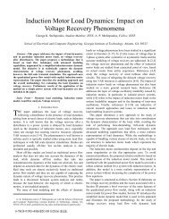
and thus the probability of flashover. Figure 1.1 shows the picture of a naturally contaminated
silicone rubber insulator. It can be seen that the pollution level is high enough for causing a
change in the natural color of the insulator.
Figure 1.1: Picture of a naturally contaminated silicone rubber insulator
The economic impact that insulator flashovers exert can be severe. For example, a power outage
for a quarter of a second in a paper industry would result in considerable downtime and
equipment damage of up to $50,000 [4]. Figure 1.2 shows the picture of a severe case of
flashover of an insulator [5].
2

Figure 1.2: The picture of a flashover of an insulator [5].
1.3 NATURE OF CONTAMINANTS
In practice, there are actually various types of contaminants that tend to settle on the insulators.
These contaminants can be classified as soluble and insoluble. Insulators that are located near
coastal regions are typically contaminated by soluble contaminants, especially NaCl (Sodium
chloride). Insulators that are located near cement or paper industries are typically contaminated
by a significant amount of non-soluble contaminants. Some of the contaminants include calcium
chloride, carbon and cement dust. Irrespective of the nature of the contaminant, flashover can
occur as long as the salts are soluble enough to form a conducting layer on the surface of the
insulator. In order to quantify the contaminants on the surface of the insulators, the soluble
contaminants are expressed in terms of Equivalent Salt Deposit Density (ESDD), which
correlates to mg of NaCl per unit surface area. Non-soluble contaminants are expressed in terms
of Non-Soluble Deposit Density (NSDD), which correlates to mg of kaolin per unit surface area.
3

Apart from the above listed sources, salts that are used for de-icing streets, roads and
sidewalks during winter to keep them safe for driving and walking add to the contamination
problem. Salt works by lowering the freezing point of water. Ice forms when the water
temperature reaches 0°C. When salt is added the temperature at which water freezes drops. A
10% salt solution freezes at -6°C, and a 20% solution freezes at -16°C. There are various road
salts like sodium chloride, calcium chloride, potassium chloride, Calcium Magnesium Acetate
(CMA), and magnesium chloride. Of these the most commonly used road salts are sodium
chloride and calcium chloride. An assessment on the quantity of road salt used every year stated
that in USA about 15 million tons and in Canada about 5 million tons of road salt is used [6, 7].
Sodium chloride, also known as rock salt, is one of the most commonly used ice melters.
Compared to other materials, it has only limited effectiveness in times of very low temperatures.
The main limitation is it will not melt ice at temperatures below -7°C. On the other hand,
calcium chloride is actually liquid in its natural state (easy to apply) and can be converted into a
dry material by removing the water. It quickly absorbs moisture from the atmosphere, while
sodium chloride must come in direct contact with moisture, which is not present at low
temperatures. Also, when calcium chloride is converted into liquid brine, it gives off heat.
Therefore, calcium chloride will melt ice at temperatures as low as -15°C. Cost may be one of
the prohibiting factors in the use of calcium chloride compared to sodium chloride [6, 7].
When applied, these road salts tend to be deposited on the surface of the insulators by the
effect of wind and the movement of the vehicles. The effect that these road salts have on the
insulators depends on the physical state by which they are applied to the road. Deicing streets by
using liquid form of salt is the newly followed practice and is expected to have the worst effect
on insulator performance.
1.4 IMPORTANCE OF SURFACE RESISTANCE MEASUREMENT (NCI)
Flashover prediction based on ESDD measurement alone may not be the best method for NCI
due to its hydrophobic nature. A hydrophobic surface can have high levels of ESDD, yet the
leakage current can be negligible as water formation on such a surface is in the form of discrete
droplets as opposed to a continuous film. An alternate method to characterize the electrical
performance was introduced based on the measurement of surface resistance under wet
conditions. The use of surface resistance for predicting the flashover voltage (FOV) is explored
in this work. To date there has not been much work done in characterizing the values of surface
resistance that would be indicative of either flashover or withstand. It is also understood that the
type of fog and rate of wetting of the insulators affects the surface resistance of NCI. It is much
easier to measure ESDD than surface resistance. Thus there is a need to determine the correlation
between ESDD and surface resistance. Studies have also found that the silicone rubber insulators
have a higher surface resistance over the EPDM insulators. The guidelines for surface resistance
measurements in laboratories under various possible test conditions are well defined [8, 9].
4

1.5 NEED FOR WORK IN FLASHOVER PREDICTION (ESPECIALLY FOR NCI)
In the USA, presently, non-ceramic materials are used extensively for termination of distribution
cables. Currently, non-ceramic insulators have captured the power market to about 35% of the
transmission line system. The increasing demand for the use of polymeric insulators and their
relatively less on field experience compared to porcelain triggered the need for more research in
this area. It should be noted that at present there are no standardized tests for understanding the
contamination flashover performance of polymeric insulators. Based on these facts it is of utmost
importance to devise an improved method to predict the FOV of an insulator based on the level
of contamination.
For new construction, relevant field experience may not be available and laboratory
experiments are often time consuming and expensive. A good theoretical model for simulating
the flashover process is a big asset as it helps minimize experimental efforts. This research is
therefore aimed at developing models by which the FOV based on contamination are to be
predicted and the dynamics of flashover to be explained in cases of both highly and nonuniformly
contaminated insulator.
5

2. FLASHOVER THEORY, EVALUATION AND MEASUREMENT OF
CONTAMINATION
2.1 FLASHOVER MECHANISMS - GENERAL THEORY AND OBENAUS MODEL
During wet atmospheric conditions like light rain or fog the contamination layer on the surface
of the insulator gets wet and promotes leakage current flow along the surface. The heat
dissipated due to the flow of leakage current evaporates the moisture on the surface of the
insulator. This evaporation leads to the formation of areas termed as “dry bands.” Dry bands tend
to form near the surface of the insulator parts where the diameter is the smallest, because of the
high current density in those parts. A concentration of voltage stress is formed around the dry
bands as the surface resistance of the dry bands is much higher than the conductive contaminated
surface film. Subsequently the dry band will break down causing an initial partial arc over the
surface. After the formation of a partial arc the propagation of the arc further depends on if E p >
E arc , that is the arc will propagate if the voltage gradient ahead of the arc, which is the voltage
gradient of the pollution layer, is greater than that of arc gradient. This is due to the fact that
ionization of the path ahead of the arc by the increasing current at every instant enables the arc to
proceed. When the arc propagation across the contaminated layer bridges the whole insulator a
flashover will occur. The flashover triggers a power arc that results in the interruption of power
supply and may damage the insulator temporarily or permanently, depending on the severity of
flashover [10 - 16].
Though the study of the process of contamination flashover has been done for many
decades at different labs and at outdoor locations across the world, the understanding of the
physical process is not complete even now. This can be attributed to the intense complexity
involved in the flashover process. Also, the numerous parameters involved in the process of
flashover make it even more difficult to understand the process completely. As an example it has
been observed in service that FOV depends upon various factors but is not limited to such as, the
polarity of voltage, particle size, non-uniform wetting, the size and nature of the pollutant surface
conductivity, wind, washing, length, orientation, diameter and profile of the insulator.
Obenaus was the first to propose a model for contamination flashover. Obenaus outlined
the steps that were required to calculate the FOV [12]. The actual computation was completed by
Neumarker who derived an expression that relates FOV and surface conductivity [13]. In this
theory flashover process is modeled as a discharge in series with a resistance as shown in Figure
2.1. Here the discharge represents the arc bridging the dry band, and the resistance represents the
un-bridged portion of the insulator. The voltage drop across the resistance is taken as a linear
function of current. The equations derived for critical voltage gradient (E c ) and critical current
(I c ) are [17-20],
E c = N (1/ (a+1)) * R p
(a/ (a+1))
(1)
I c = (N/R p ) (1/a+1) (2)
6

where
R p = R poln / (LD-Larc), uniform surface resistance per unit length of the pollution layer
N = Reignition constant
a = Arc equation exponent
R poln = Series resistance of the pollution layer
LD, Larc = Leakage distance and arc length respectively.
Figure 2.1: Obenaus model of polluted insulator [10]
2.2 FLASHOVER THEORY OF VARIOUS OTHER RESEARCHERS
Various other researchers have proposed alternative models to that of Obenaus. Hampton
proposed a theory on the basis of an experiment in which he used a water jet to simulate a
contaminated long rod insulator [14]. According to Hampton’s theory, FOV was treated
primarily as a stability problem. Hampton stated that an unstable situation occurs if there is a
current increase when the discharge root is displaced in the direction of flashover. From this he
concluded that if the voltage gradient along the discharge was ever to fall below the gradient
along the resistive column, then flashover would occur. Subsequently it was mathematically
proven by Hesketh that Hampton’s two criteria of voltage gradient and current increase were
identical only in the case of a long rod insulator [15].
Alston and Zoledaiowski later on proposed an algebraic derivation for the critical
conditions of flashover [16]. They incorporated the discharge length in the condition of
flashover. According to their theory the voltage required to maintain local discharges on polluted
insulators may increase with an increase in discharge length. If this voltage exceeds the supply
voltage then the discharge extinguishes without causing a flashover. An equation was proposed
that defines the critical relation between the applied stress and the resistance of the pollution for
DC voltages. According to the equation, flashover cannot occur if:
E c < 10.5 * R poln
0.43
(3)
7

Numerous authors who worked in this field proposed various equations by varying the empirical
constant, and calculations of FOV based on each model yielded a different value. Rizk proposed
a similar equation for AC voltages which is given by [17],
E c < 23 * R poln
0.40
(4)
In Equation (4) the increase in the constant of proportionality is attributed to the arc
extinction due to natural current zeroes, which inhibits arc elongation.
Most of the models studied so far are static in nature in the sense there is no arc
propagation criterion accounted for in these models. The static models assume that once the arc
is initiated it propagates unextinguished. Thinking in terms of reality, arc propagation is a rapid
time varying phenomena, an arc will propagate only when conditions are conducive. Static
models do not consider variations in arc and pollution resistance and arc current with time. These
limitations in static models led to the development of dynamic models.
The dynamic model was initially proposed by Jolly, Cheng and Otten [19]. In this model
the arc propagation criterion used was the variation in arc electrode gap. With this model it was
possible to predict the time to flashover for electrolyte strips. Even though a good correlation
was observed on one dimension, it was defective for 2D and 3D. Subsequently, various authors,
including Rizk, proposed dynamic models. However significant improvement in the
development of a dynamic model was undertaken by Raji Sundararajan. In her work the various
factors like arc propagation criteria, change in arc parameters with time, effect of various
contaminants on flashover and the role of geometry, were all considered [20].
2.3 FLASHOVER THEORY IN PARTIALLY CONTAMINATED INSULATORS
Apart from the various theories discussed so far regarding a uniformly contaminated insulator,
flashover, was observed also in a partially or a non-uniformly contaminated insulator. In many
insulators flashovers have taken place without any indication of surface discharge activity. The
FOV is much lower than predicted by clean fog. High non-uniform voltage distribution is
believed to trigger streamer discharges. Some significant observations in this type of flashover
termed as sudden flashover are [21- 24]:
• In streamer discharge FOV is non-linear to leakage distance.
• The high resistance region near the HV end causes higher field intensification
• Insulators with smaller shed spacing suffered a significant reduction in
performance as smaller shed spacing may itself aid an arc to jump
• In contrast to wholly contaminated insulators the path of the arc is essentially
through air instead of following the leakage distance path
• Hanging water droplets due to rain may substantially reduce dielectric strength
between sheds
• Complete shed bridging due to water bridging the gap
• Ratio of the resistance/unit length of wet region to dry region is a key parameter
for prediction
8

Some possible solutions that are sought of for this problem include but are not limited to:
• Insulator shapes are to be modified with the aim of an improved contamination
performance
• Improvement of insulator materials improves the performance (NCI better than
ceramic)
• Increase in shed spacing as typically observed in NCI
2.4 MEASUREMENT OF CONTAMINATION SEVERITY
Contamination severity on the surface of insulators can be given in terms of ESDD as explained
earlier. The measurement of ESDD in case of porcelain and glass has been standardized in the
International Electrotechnical Commission (IEC) document 60507
ESDD is measured by dissolving the contaminants on the surface of the insulators, in
deionized water and then measuring the conductivity of the water. The ESDD is then calculated
using the following formula
σ 20 =σ ө (1 – b (ө - 20)) (5)
σө - The measured conductivity in S/m.
b - 0.01998 (constant)
ESDD = (5.7 * σ 20 ) 1.03 * VO / AR (6)
VO- Volume of dissolvent (distilled water) in m 3
AR– Area of the insulator surface in m 2
This method is observed to be good for measuring ESDD for porcelain and glass insulators, as
these are completely wettable [9].
2.5 EVALUATION OF CONTAMINATION FLASHOVER PERFORMANCE IN
LABORATORIES
The properties of polymer insulators tend to change with time because of longtime exposure to
UV (Ultra Violet) rays from sunlight, temperature, mechanical loads and electrical discharges in
the form of arcing or corona. Such a reduction in the electrical and mechanical properties is
termed aging. The silicone rubber insulators tend to lose one of their most important properties
of hydrophobicity when they are continually subjected to various extreme levels of
environmental factors. The various characteristics of the insulators can be evaluated by the
records obtained from service. Though the records from the field are of immense value, they are
difficult to obtain and may take a long period of time before their validity can be proved. As a
result laboratory tests are increasingly used to evaluate the various performance characteristics of
the insulators to correlate with actual field conditions.
9

Laboratory results are used by most of the manufacturers to determine the design and
material selection of insulators. They are used by transmission engineers to determine the design
of transmission lines and the insulators to be used on those lines. The most common tests that are
employed for the evaluation of non–ceramic insulators are the clean fog and salt fog test. These
tests are standardized for ceramic insulators and are referred to as fog chamber tests.
The clean fog chamber tests involve the pre-contamination of the insulator with slurry
made of conductive salt usually sodium chloride and an inert clay binder (kaolin). Then the
insulator is subjected to wetting by steam. This simulates the field condition in which the
insulator is first contaminated and then wetted. In the case of a salt fog test a clean insulator is
energized in the fog chamber using fog produced from saline (NaCl) water. This test simulates
the field condition in which the clean insulator is subjected to contamination in a salty
environment as it happens in coastal areas. The service condition can be varied by the applied
voltage, the rate of wetting and the amount of contamination, depending on the requirement. All
these parameters are observed to have significant effect on the performance of the insulator.
2.6 SURFACE RESISTANCE FOR CHARACTERIZING FLASHOVER
The measurement of surface resistance in the case of non–ceramic insulators during wet
conditions is a useful technique to characterize the contamination performance and aging.
Silicone insulators, due to their hydrophobic nature, may perform satisfactorily during wet
conditions. In those cases the surface resistance, calculated from the leakage current measured,
acts as a true representative of the contamination performance of the insulator. In reality surface
resistance has been used as a key parameter to model flashover. One example of such a model
assumes a dry zone of varying length, which is used to determine the conditions that may lead to
flashover in HVDC (High Voltage Direct Current) wall bushings in non-uniform rain. In this
model the ratio of the resistance per unit length of wet region to dry region is used as a key
parameter. Surface resistance measurements can be utilized to evaluate the potential capability of
various materials to prevent HVDC wall bushing flashover in conditions of non-uniform rain.
The above model which analyzed the voltage distribution across wet and dry zones, accounts for
the breakdown strength of the dry zones leading to the following necessary condition for
flashover in HVDC wall bushing [22]:
(R WO / R DO ) < (V S / E O L B ); where
R WO and R DO are the resistance per unit length of wet and dry regions respectively
E O is the breakdown strength of the dry region, L B is the total bushing length.
Surface resistance generally reflects multivariables, which are typically the type of
material, wetting rate, ESDD and the recovery characteristic. The surface resistance of the
insulator that has recovered is different from the surface resistance of the un-recovered insulator
particularly for the silicone rubber type. Apart from these, surface resistance can be used to
assess the aging of the insulating materials. Aging of insulating materials can be defined
according to IEC and IEEE standards, as the ‘occurrence of irreversible deleterious changes that
critically affect performance and shorten useful life.’ Aging is a complicated process. Aging
would lead to increased leakage current and subsequent flashover of insulators during wet and
10

contaminated conditions. Quantifying and comparing aging in non – ceramic insulators is not a
simple task. As aging leads to increased leakage current, it can be assumed that surface
resistance measurements can be used as indicators to quantify and compare aging in case of NCI.
A task force of the IEEE working group on insulator contamination by R. S. Gorur, et al
[9] determined whether surface resistance measurements can be formalized to ensure repeatable
and reproducible results for both silicone and EPDM. A porcelain post insulator was used as a
reference for the analysis. For the above study surface resistance was measured both in
artificially contaminated and in “as received” conditions. Fog wetting and spray wetting were the
methods of wetting used. The study finally concluded that it is possible to establish a standard
for surface resistance measurements in the laboratories. The study also issued useful guidelines
for surface resistance measurements like insulator orientation, voltage to be applied, duration of
test and method of wetting.
11

3. EXPERIMENTAL SET UP
3.1 FOG CHAMBER DESCRIPTION
The experiments in this research work involved the estimation of ESDD, measurement of surface
resistance and estimation of flashover of porcelain and polymer insulators namely silicone rubber
and EPDM. The fog chambers are in general used for various artificial contamination tests of
porcelain, glass and non-ceramic insulators under different simulated environmental conditions.
Various experiments were carried out in the fog chamber available at the high voltage laboratory
in ASU.
The fog chamber used for these experiments is made of stainless steel sheets and its
dimensions are 3.66 X 3.05 X 2.44 m which makes it a volume of approximately 27 m 3 . There
are four IEC dimensioned fog nozzles present, one on each wall of the chamber inside. The HV
supply is provided by a transformer rated at 40 kVA/100 kV located outside the fog chamber. A
water boiler is located inside the fog chamber for the generation of steam fog. The water source
for the air nozzle is a water drum outside the chamber. The condensed water inside the chamber
is circulated out to the drain using a pump that is operated by a timer by which water can be
pumped out every 15 minutes. For the visual observation of the fog chamber a 30 X 20 cm glass
window is fitted on the door.
Three different modes of fog generation that are available for the experiments are:
1) Salt fog generated by the standard IEC 507 nozzles
2) Steam fog generated by the boiler that is inside the chamber
3) Fog generated by ultrasonic fog generators.
The water is boiled in a vat to produce a steam input rate of about 50 - 250 g/m 3 /h. In this
work ultrasonic nebulizers were used to generate fog. The size of the droplet generated by the
nebulizer is very small typically 1 micron in diameter. These devices are easy to maintain,
consume less power and minimize corrosion problems encountered with conventional fog
generators like boiling water or salt spray. A relative humidity level of 100% was achieved
within 20 minutes of energizing the fog generators.
3.2 ARTIFICIAL CONTAMINATION OF NON CERAMIC INSULATORS
An examination of insulators that were in the field for a long time and exposed to various
contaminants indicates that the contamination is dispersed fairly uniformly. Based on this it is
important to make sure that a uniform layer of contamination is applied on the insulators for the
experiments. The contamination slurry to be applied on the insulator is obtained by mixing 40g
of kaolin in one liter of deionized water. Kaolin acts as the binder in the slurry. No other wetting
agent is used in the slurry, as it may affect the surface characteristics of the non-ceramic
insulator. An appropriate amount of NaCl was added to the slurry depending on the level of
ESDD to be obtained. Using brush a uniform coating of contamination was applied on the
insulator. If the required level of ESDD is not obtained from the process, then the process is
12

epeated again with further addition of sodium chloride to the slurry and reapplication on the
insulator to get the required ESDD. There was several hours elapsed from the time the surface
was dry to the time at which they were tested. This allowed recovery of hydrophobicity of
silicone rubber to various degrees depending on the time elapsed. Samples were tested when the
surface had no recovery of hydrophobicity (1 hour after drying), and visibly recovered its
hydrophobicity (3 days after drying). Recovery was judged by spraying water and noting if the
surface wetted out or beaded in to small drops and conclusions were made based on STRI guide
92/1. The EPDM samples were always hydrophilic and there was no visible recovery of the
hydrophobicity with time.
3.3 MEASUREMENT OF SURFACE CONDUCTIVITY AND CALCULATION OF ESDD
After the artificially contaminated insulators are dried, the surface conductivity is to be measured
to calculate the ESDD. A compact portable contamination measurement unit is used to measure
the conductivity on the surface of the insulator. It basically consists of a measurement cell
mounted on a vise grip that can be fixed on most of the insulator surfaces. The measurement cell
is made of a plexiglass tube that is sealed with an O-ring at the lower perimeter to make it water
tight when it is fixed on the surface of insulator. The surface area of the measurement cell is
approximately 1.8 cm 2 .
The conductivity of the insulator surface where the instrument is placed is measured as
follows:
1) The portable device is fixed on the surface of the insulator and is filled with 1.8 ml of
deionized water.
2) The deionized water is allowed to remain on the surface of the insulator for about two
minutes. After two minutes the water is siphoned off using a syringe and this is again
siphoned onto the surface so that the contaminant dissolves properly. This process is
repeated for about five times to get an accurate assessment of conductivity.
3) The conductivity of the removed water is then measured using a calibrated digital
conductivity meter (B-173).
4) This whole process is repeated on different insulator sheds to ensure that insulators
have been contaminated uniformly.
5) ESDD is then calculated from the measured conductivity using the formula explained
earlier in section 2.4
The conductivity meter used (B-173) has a digital LCD that indicates the conductivity
directly. The conductivity meter can be used to measure a wide range of conductivity varying
from 0 – 19.9 mS/cm. The conductivity meter is rinsed in the washing liquid (purified water) and
calibrated periodically using a standard solution of 1.41 mS/cm. in order get accurate
measurements.
13

3.4 TESTING PROCEDURE FOR SURFACE RESISTANCE MEASUREMENT AND
ESTIMATION OF FOV
AC voltage in the range of 2-4 kV was used depending on the insulator material and dimensions.
The voltage was applied across aluminum tape electrodes that were placed in between the
insulator hardware. The leakage distance of the insulators between the electrodes was typically
15 cm. The voltage applied should be adequate to establish a measurable leakage current but not
high enough to initiate discharges. The insulators were mounted vertically in the chamber. Figure
3.1 shows the schematic of testing. Care is taken to ensure that the source of fog generation is not
directly beneath the sample. The data acquisition system for the leakage current consists of an
oscilloscope in which there are three options of resistance 100 Ω, 470 Ω and 1 kΩ. The leakage
current is measured as a voltage drop across the resistor connected in series with the sample. The
surface resistance is calculated based on the fact that the applied voltage is the sum of the voltage
drop across the sample and resistor. The surface resistance value is high initially and a steady
value of surface resistance was obtained in 70-90 minutes after starting the fog generators
HV power supply
Ultrasonic
nebulizers
Shunt
Test insulator
Figure 3.1: Schematic of testing in fog chamber for surface resistance measurement
Most of the experiments performed in this work measured the surface resistance of different
samples at different values of ESDD. Moreover, FOV for different levels of ESDD were
estimated. To measure FOV, the insulator is subjected to 80% of the probable FOV (determined
from previous trials) for 20 minutes after the relative humidity has reached 100%. If there is no
flashover the voltage is raised in 10%, and each step is maintained for 5 minutes until flashover
is obtained. This process is repeated for different levels of ESDD. The FOV reported is the
average of three measurements for the same ESDD. A different sample of the same type was
used for different trials.
14

4. RESULTS AND ANALYSIS
4.1 COMPARISON OF SIMULATED RESULTS OF VARIOUS ARC MODELS
As discussed in Section 2.2 there are numerous models that have been proposed for predicting
the FOV. Various researchers have proposed numerous models based on different empirical
values for constant and exponent of static arc characteristic. In order to investigate how close the
predictions are by different authors, various models were simulated by keeping Sundararajan
model (Researcher A) as the basis of comparison [18, 20, 25]. The simulation results for DC and
AC models are presented in Table 4.1 and Table 4.3 respectively. The E arc and E p equations used
by different researchers for DC is given in Table 4.2 and for AC in Table 4.4. The dimensional
details of the standard IEEE porcelain bell considered for simulation are leakage length of 28 cm,
shed diameter of 25.4 cm and unit spacing of 14.6 cm. The equations that were used as basis for
simulation for DC models (equations 7 and 8), AC models (equations 7 and 9) are given as
−n
Earc
= N × I
(7)
1
a
E = = a 1 × a+
1
p Ec
A rpu
(8)
n
n
n
−
+ 1
= = 10* × ( − ) + 1 × + 1 ×
rpu n
E E N N A n n n
p c
(9)
n + 1
Where
n- Reignition exponent (typically 0.5)
A- Arc constant (typically 0.15 * N)
I - Current entering the pollution layer
rpu - average resistance per unit length
The Matlab programs that were developed based on the flowchart developed by Sundararajan for
these simulations are given in Appendix titled “Matlab programs” [10, 20]. The values of the
various constants and the arcing model equations that were used for simulations are from
references [10, 18, 20, 25] and are provided in the Appendix. It can be inferred from Table 4.1
that the variation of prediction for FOV is a very wide range from 0% to as high as 170%. In
case of AC models with Rizk’s model (Researcher E) as reference for comparison the variation
of prediction for FOV is from 2% to about 90%. Hence, it can be observed that there is a very
wide range of prediction and it is very difficult to predict the exact FOV.
15

Table 4.1. Comparison of simulated FOV prediction of a standard IEEE porcelain
Bell based on different models (DC)
ESDD
(mg/cm 2 ) Researcher A Researcher B Researcher C Researcher D
Light (kV) (kV) (kV) (kV)
0.01 14.6 12.0 14.2 28.0
0.02 11.8 11.0 11.8 24.6
0.03 10.4 10.4 10.6 22.8
0.04 9.6 10.0 9.8 21.6
Moderate
0.05 9 9.8 9.2 20.8
0.06 8.5 9.6 8.8 20.2
0.07 8.1 9.1 8.4 19.6
0.08 7.8 9.2 8.2 19.0
Heavy
0.10 7.3 9.0 7.8 18.4
0.12 6.9 8.8 7.4 17.8
0.15 6.5 8.6 7.0 17.0
0.20 6.0 8.2 6.4 16.2
Table 4.2. E p and E arc used by different researchers (DC)
Researcher A Researcher B Researcher C Researcher D
E p (V/cm) 15.83*Rp 0.4 28.5*rpu 0.43 20.1*rpu 0.296 24.58*rpu 0.194
E arc (V/cm) 63*I (-0.5) 37.2*I (-0.5) 15.93*I -0.42 312.7*I -0.24
16

Table 4.3. Comparison of simulated FOV prediction of a standard IEEE porcelain
Bell based on different models (AC)
ESDD
(mg/cm 2 ) Researcher E Researcher F Researcher G Researcher H
Light (kV) (kV) (kV) (kV)
0.01 12.0 20.2 12.2 22.6
0.02 10.6 16.2 10 18.2
0.03 9.8 14.2 8.8 16
0.04 9.2 13.0 8.0 14.6
Moderate
0.05 9.0 12.2 7.6 13.6
0.06 8.6 11.6 7.2 13.0
0.07 8.4 11.0 6.8 12.4
0.08 8.2 10.6 6.6 11.8
Heavy
0.10 8.0 9.8 6.2 11.0
0.12 7.6 9.4 6 10.4
0.15 7.4 8.8 5.6 9.8
0.20 7.0 8.0 5.2 9.0
Table 4.4. E p and E arc used by different researchers (AC)
Researcher E Researcher F Researcher G Researcher H
E p (V/cm) 58*rpu 0.4 103.3*rpu 0.33 63.4*rpu 0.333 113.6*rpu 0.333
E arc (V/cm) 59*I (-0.5) 80*I (-0.5) 37.78*I -0.5 94*I -0.5
4.2 ANALYSIS OF TEST RESULTS OF DIFFERENT ROAD SALTS
As mentioned earlier, road salts, which are applied for deicing purposes, get deposited on the
insulator and considerably deteriorate the performance. In order to study their effect, three types
of salts namely solid calcium chloride, solid sodium chloride and liquid calcium chloride were
considered. As a first assessment, the time taken by each salt to reach a stable comparable
conductivity was noted. A graphical variation of time taken to reach stable conductivity values
for different salts is shown in Figure 4.1. From observing Figure 4.1 it can be expected that once
the road salts get deposited onto the surface of insulators the liquid salt will have considerable
effect in early stages compared to other salts. To confirm this, they were applied on a standard
porcelain bell of dimension (5.7” X 10”) of leakage length 12.2”. All the three samples were
tested at an ESDD of 0.17 mg/cm 2 and the surface resistance was measured as shown in Figure
4.2. The applied voltage was 2 kV in all the cases. In Figure 4.2 the Y axis represents surface
resistance measured in MΩ per cm of leakage distance. It can be observed that application of
17

liquid salts on the road has an immediate, more deleterious effect than other salts. The liquid salt
has enough moisture resulting in an immediate lower surface resistance whereas for solid salts it
requires some time to acquire. Figure 4.3 shows the FOV calculation for a single standard
porcelain bell (5.75” X 10”) with a leakage distance of 310 mm. It can be observed that at the
starting point there is a 56% decrease in FOV with liquid salt compared to solid CaCl 2 , and 28%
decrease in FOV compared to solid NaCl. This fact quantitatively substantiates the deleterious
effect of liquid salt on flashover performance
Conductivity (mS/cm)
1.8
1.6
1.4
1.2
1
0.8
0.6
0.4
0.2
0
Liquid calcium chloride
with water
0 50 100 150 200
Time (seconds)
Solid calcium chloride
with water
Solid sodium chloride with water
Figure 4.1: Time taken to reach stable conductivity values for different salts
18

1.20
Surface resistance (Mohm/cm)
1.00
0.80
0.60
0.40
0.20
Solid sodium
chloride with water
Liquid calcium chloride
with water
Solid calcium chloride
with water
0.00
0 20 40 60 80 100
Time of wetting (minutes)
Figure 4.2: Variation of surface resistance with time for the three salts
FOV (kV)
18
16
14
12
10
8
6
4
Solid sodium chloride with water
Solid calcium chloride with water
0 20 40 60 80 100
Liquid calcium chloride with water
Time of wetting (minutes)
Figure 4.3: FOV prediction for a single standard porcelain bell (5.75”X 10”) with 310 mm
leakage distance artificially contaminated with different salts at an ESDD of 0.17 mg/cm 2
In order to understand the effect of shed bridging on further lowering the FOV different
scenarios as shown in Figure 4.4 were considered for FOV prediction
19

Figure 4.4: Schematic of leakage length path shown in dotted line when there is no shed
bridging (a), one shed bridging (b) and two sheds bridging (c)
Figure 4.5 shows the predicted FOV of 305” leakage distance post for liquid calcium chloride
considering shed bridging effect. It can be observed that while the insulator is not expected to
flashover in normal operating conditions whereas with three shed bridging it will flashover.
Figure 4.6 shows the predicted FOV of 132” leakage distance post with solid calcium chloride
and solid sodium chloride salts as contaminants. With the nominal operating voltage of 230 kV
the insulator is expected to withstand and not flashover if solid calcium chloride is the
contaminant but will flashover if solid sodium chloride is the contaminant. Thus it is evident that
the performance of insulators with solid calcium chloride is much superior to solid sodium
chloride salt. The simulations to obtain graphs of Figs 4.5 and 4.6 were done in Matlab.
FOV (kV)
146
141
136
131
No shed bridge
3 shed bridge
0 2 4 6 8 10 12 14 16
Nominal operating voltage
of 230 kV system
1 shed bridge
Time of wetting (minutes)
2 shed bridge
Figure 4.5: Predicted FOV of 305” (1550 kV BIL) leakage distance post with liquid calcium
chloride as contaminant with shed bridging effect (ESDD of 0.17 mg/cm 2 )
20

200
Solid calcium chloride with water
150
Nominal operating voltage of 230 kV system
FOV (kV)
100
50
Solid sodium chloride with water
0
0 5 10 15 20 25
Time of wetting (minutes)
Figure 4.6: Predicted FOV of 132” (750 kV BIL) leakage distance post with solid calcium
chloride and solid sodium chloride salts as contaminants
4.3 EFFECT OF WATER DROPLETS IN DIFFERENT SHEDS
In order to further understand, the intensification of E-field at the tip of junction of water droplet
and shed was modeled using coulomb. Two cases were considered. First is the change in E-field
with the increase in number of water droplets in a same shed. Secondly, considering the same
scenario in subsequent sheds (away from HV end). The results obtained for the geometry of a 5
shed insulator with leakage distance 133.5 cm, shed diameter 12 cm, and a shed spacing of 10
cm is given in Table 4.5. The radius of water droplet considered was 0.25 cm.
Shed
Position
Table 4.5. Effect of water droplets in different sheds
Number of
water
droplets
E field increase in% compared to
no water droplet
First shed One droplet 33.33
(closest to
HV
end)
Four droplets 85.55
Second shed One droplet 6.1
21

Following are the observations from Table 4.5.
• In any shed the increase in number of water droplets shows an increase in E- field at the
tip of the shed
• As we move away from the HV end towards ground end the increase in E-field value at
the water droplet/shed junction is significantly lower than observed for the shed which is
closest to HV end.
4.4 DEVELOPMENT OF A MODEL TO PREDICT FOV BASED ON ESDD
VARIATION FOR NON-CERAMIC AND CERAMIC INSULATORS
In order to understand the effect of variation of ESDD to FOV, a series of experiments were
performed on new and field-aged samples of insulators using silicone rubber and ethylene
propylene diene monomer (EPDM) rubber as housing materials. The insulator shapes were
identical. Porcelain line post insulators with a geometry as close to that of the NCI was used as a
reference. The field-aged samples were removed after 5 years of exposure in the mid west USA.
It is important that the period of field exposure and the service location be similar for comparison
of different material types. The aged silicone samples were still hydrophobic but the EPDM
samples had lost its initial hydrophobicity. The hydrophobicity was assessed visually by using
STRI guide 92/1. There was surface discoloration of the aged EPDM samples most likely from
ultraviolet radiation in sunlight. There was no visible degradation on the aged samples. The
experiments were performed with ESDD values as low as 0.08 mg/cm 2 to 0.34 mg/cm 2 . The
dimensional details of the samples tested are provided in Table 4.6. Figure 4.7 shows the
experimental results for the variation of ESDD vs FOV for all the four material types. It can be
seen that for the same level of ESDD the FOV for an aged silicone rubber is about 12% less
compared to new silicone rubber. The aged EPDM has a FOV of about 16% lower than aged
silicone rubber, whereas porcelain has a FOV of about 16% lower than aged EPDM. These
differences in the FOV are indicative of inherent differences in the materials’ ability to resist
water filming.
Table 4.6. Dimensional details
Type of material Leakage
distance
(cm)
Shed
diameter
(cm)
Shed
spacing
(cm)
New silicone rubber 27.0 9.0 3.0
Aged silicone rubber 27.0 9.0 3.0
Aged EPDM 26.0 9.0 2.0
Porcelain 25.0 13 2.0
22

FOV( kV)
30.00
25.00
20.00
15.00
10.00
5.00
0.00
Aged
silicone
New silicone
Porcelain
0 0.1 0.2 0.3 0.4
ESDD (mg/sqcm)
Aged
EPDM
Figure 4.7: Variation of FOV to ESDD for different materials
Although most of the tests have been made at very high levels of ESDD it is possible to fit a
regression model and predict with a high prediction interval of 95% the FOV for low levels of
ESDD where experiments cannot be performed. Even though, in general it might be a risk to
extrapolate, if the fitted regression model can be validated at some point where it has been
extrapolated it can be considered to be a valid model. A regression model was initially developed
for new silicone rubber material considering data points for ESDD ranging from 0.12 – 0.32. The
developed regression model is valid only when certain assumptions are true. The basic
assumptions to be checked are:
• Errors are normally distributed – Checked through normal probability plot of residuals
• Errors have zero mean and constant variance – Checked through plot between residuals
and predicted values
• Errors are uncorrelated – Checked through plot between residuals and run order.
With regard to normal probability plot of residuals, the residuals should lie approximately in a
straight line. If that is so, then it can be inferred that there is no considerable deviation from
normality. Typically, a random scatter of points is obtained when the assumption of constant
variance is satisfied. That is, the plot between the residuals and predicted values should not
indicate any specific shape. In the plot, between residuals and run order there should not be any
trend discernable from the plot. If so, the assumption of independence of errors is not violated
All the assumptions were checked and found satisfied and hence the developed model is a valid
model [26 27]. Details of the data set for this model and for various models that follow this and
the graphs to support assumptions for all the models are listed under Appendix – Data set.
23

a) New silicone rubber housing
Regression Analysis: FOV versus Ln (ESDD) for new silicone rubber
The regression equation is
FOV = 10.2 - 6.02 Ln (ESDD)
Predictor Coef SE Coef T P
Constant 10.1983 0.4162 24.50 0.000
Ln (ESDD) -6.0235 0.2599 -23.18 0.000
S = 0.330449 R-Sq = 97.8% R-Sq(adj) = 97.6%
PRESS = 1.75952 R-Sq(pred) = 97.07%
Analysis of Variance
Source DF SS MS F P
Regression 1 58.658 58.658 537.18 0.000
Residual Error 12 1.310 0.109
Lack of Fit 3 0.644 0.215 2.90 0.094
Pure Error 9 0.667 0.074
Total 13 59.969
Where
SE coef – Standard error coefficient
T – Standard “T” Statistic
P – Probability of testing the significance of null hypothesis
F- Standard “F” statistic
S – Standard deviation
PRESS – Prediction error sum of squares
R 2 – Residual sum of squares
R 2 (adj) –Adjusted residual sum of squares
R 2 – (pred) - Predicted residual sum of squares
DF – Degrees of freedom
SS – Sum of squares
MS – Mean sum of squares
In general a high value of R 2 (adj), indicates that the model is capable of explaining the
variability in a wide range. A high value of R 2 (pred) indicates the capability in predicting the
variability in new observations and is correlated with a low value of PRESS. A high “F” ratio
and low “p” value means that the model is highly significant [26 27]. In order to validate the
model in the region of extrapolation a data point - ESDD of 0.08 was considered.
24

Predicted Values for New Observations at 95% Prediction Interval = (24.49 kV, 26.33 kV)
From Experiment = 24.5 kV
Thus the experimentally obtained value is observed to be within the range of 95% prediction
limits and thus the model is validated. Figure 4.8 shows the FOV prediction at 95% prediction
interval for new silicone rubber where in there are two sections, one is the experimental data
from ESDD 0.12 to 0.32 mg/cm 2 and the other is the projected/validated region from ESDD 0.11
to 0.04 mg/cm 2 in one side and from 0.35 to 0.45 mg/cm 2 on the other side. In Figure 4.8 CI
represents confidence interval, PI the prediction interval, LL the lower limit of PI and UL the
upper limit of PI. From Figure 4.8 an estimate of the range of FOV for very low values of ESDD
where actual experiments are not possible can be obtained.
31.00
Predicted/
validated
region
Experimental values
Predicted
region
28.00
FOV (kV)
25.00
22.00
Mean of LL
and UL
Mean of LL
and UL
19.00
16.00
13.00
0.00 0.10 0.20 0.30 0.40 0.50
ESDD (mg/sqcm)
Figure 4.8: FOV prediction curve at 95% Prediction interval for new silicone rubber
25

) Aged silicone rubber housing
Regression Analysis: FOV versus ln (ESDD)
The regression equation is
FOV = 7.33 - 6.52 ln (ESDD)
Predictor Coef SE Coef T P
Constant 7.3294 0.3372 21.73 0.000
ln (ESDD) -6.5165 0.2123 -30.69 0.000
S = 0.267489 R-Sq = 97.7% R-Sq(adj) = 97.6%
PRESS = 1.87678 R-Sq(pred) = 97.28%
Analysis of Variance
Source DF SS MS F P
Regression 1 67.384 67.384 941.77 0.000
Residual Error 22 1.574 0.072
Lack of Fit 6 0.407 0.068 0.93 0.499
Pure Error 16 1.167 0.073
Total 23 68.958
Figure 4.9 shows the FOV prediction at 95% prediction interval for aged silicone rubber, the
experimental data is from ESDD 0.15 to 0.32 mg/cm 2 and the projected/validated region is from
ESDD 0.13 to 0.05 mg/cm 2 in one side and from 0.33 to 0.44 mg/cm 2 on other side. In order to
validate the model in the region of extrapolation a data point - ESDD of 0.13 was considered.
Predicted Values for New Observations at 95% Prediction Interval = (20.02 kV, 21.23 kV)
From Experiment = 20.83 kV
Thus the experimentally obtained value is observed to be within the range of 95% prediction
limits and thus the model is validated.
26

Predicted
and validated
region
Experimental values
Predicted
region
27.00
23.00
FOV (kV)
19.00
Mean of LL
and UL
Mean of LL
and UL
15.00
11.00
0.00 0.05 0.10 0.15 0.20 0.25 0.30 0.35 0.40 0.45
ESDD (mg/sqcm)
Figure 4.9: FOV prediction curve at 95% Prediction interval for aged silicone rubber
c) Aged EPDM housing material
Regression Analysis: FOV versus ln(ESDD)
The regression equation is
FOV = - 9.90 ln(ESDD)
Predictor Coef SE Coef T P
Noconstant
ln(ESDD) -9.89945 0.06946 -142.51 0.000
S = 0.367873
PRESS = 2.18039
Analysis of Variance
Source DF SS MS F P
Regression 1 2748.6 2748.6 20310.33 0.000
Residual Error 14 1.9 0.1
Lack of Fit 4 1.1 0.3 3.18 0.063
Pure Error 10 0.8 0.1
Total 15 2750.5
27

Figure 4.10 shows the FOV prediction at 95% prediction interval for aged EPDM, the
experimental data is from ESDD 0.20 to 0.34 mg/cm 2 and the projected/validated region is from
ESDD 0.18 to 0.13 mg/cm 2 in one side and from 0.36 to 0.44 mg/cm 2 on the other side. In order
to validate the model in the region of extrapolation a data point - ESDD of 0.18 was considered.
Predicted Values for New Observations at 95% Prediction Interval = (16.15 kV, 17.80 kV)
From Experiment = 16.67 kV
Thus the experimentally obtained value is observed to be within the range of 95% prediction
limits and thus the model is validated
23.00
Predicted
and
validated
region
Experimental values
Predicted
region
21.00
19.00
17.00
FOV (kV)
15.00
13.00
11.00
Mean of
LL and
UL
Mean of LL
and UL
9.00
7.00
0.05 0.10 0.15 0.20 0.25 0.30 0.35 0.40 0.45 0.50
ESDD (mg/sqcm)
Figure 4.10: FOV prediction curve at 95% Prediction interval for aged EPDM
28

d) Porcelain
Regression Analysis: FOV versus ln(ESDD)
The regression equation is
FOV = - 7.84 ln(ESDD)
Predictor Coef SE Coef T P
Noconstant
ln(ESDD) -7.84361 0.06801 -115.33 0.000
S = 0.320742
PRESS = 1.01321
Analysis of Variance
Source DF SS MS F P
Regression 1 1368.4 1368.4 13301.75 0.000
Residual Error 8 0.8 0.1
Lack of Fit 2 0.3 0.2 1.94 0.224
Pure Error 6 0.5 0.1
Total 9 1369.3
Figure 4.11 shows the FOV prediction at 95% prediction interval for porcelain, the experimental
data is from ESDD 0.12 to 0.32 mg/cm 2 and the other is the projected region from ESDD 0.11 to
0.05 mg/cm 2 and in other side from 0.35 to 0.45 mg/cm 2 .
29

25.00
20.00
Lower
prediction
limit
Predicted
region
UL 95 % PI
Experimental
values
Predicted
region
Upper
Prediction
limit
FOV (kV)
15.00
10.00
Mean of
LL and
UL
LL 95% PI
LL 95% CI
UL 95 % CI
UL 95 % PI
Mean of LL
and UL
LL 95% PI
5.00
0 0.1 0.2 0.3 0.4 0.5
ESDD (mg/sqcm)
Figure 4.11: FOV prediction curve at 95% Prediction interval for PORCELAIN
4.5 DEVELOPMENT OF A MODEL TO PREDICT FOV BASED ON SURFACE
RESISTANCE MEASUREMENT FOR NON-CERAMIC INSULATORS
As mentioned earlier, measurement of the surface resistance can be considered an effective way
to analyze the condition of the insulators. The surface resistance of aged silicone rubber and
EPDM was measured for different levels of ESDD. From Figure 4.12 it can be observed that for
the same ESDD the surface resistance values are much lower for field aged EPDM than field
aged silicone rubber and this is due to the hydrophobic property of silicone rubber. The
hydrophilic nature of the EPDM can be attributed to the increase in surface energy resulting from
chemical degradation. For silicone rubber the dynamics of the hydrophobic surface results in a
much higher value of surface resistance than EPDM. The formation of a thick layer of water on
the surface of EPDM is much different than that of silicone rubber. All these factors attribute to
the difference of surface resistance values for silicone rubber and EPDM [28, 29, 32]. A
comparison of experimental results of surface resistance for a constant ESDD is shown in Figure
4.13 for field-aged silicone rubber with and without recovery, new and field aged EPDM and
porcelain. The data in Figures 4.12 and 4.13 illustrate the role played by the silicone rubber
material towards improving the contamination performance, as the surface resistance is always
higher than that of EPDM and porcelain. The actual values that were obtained for surface
resistance for different values of ESDD and the corresponding FOV have also been tabulated in
Table 6.5 in Appendix A.
30

Surface resistance (Mohm/cm)
0.9
0.8
0.7
0.6
0.5
0.4
0.3
0.2
Aged Silicone
rubber - no
recovery
Aged
EPDM
Aged
Silicone
rubber - no
recovery
Aged
EPDM
Aged
Silicone
rubber- no
recovery
Aged
EPDM
Aged
Silicone
rubber- no
recovery
Aged
EPDM
0.1
0
0.175 0.185 0.255
0.275
ESDD (mg/sqcm)
Figure 4.12: Comparison of experimental results of surface resistance vs. ESDD
for aged silicone rubber and aged EPDM
1.4
Aged silicone rubber
with recovery
1.2
Surface resistance (Mohm/cm)
1
0.8
0.6
0.4
Aged silicone rubber
without recovery
New EPDM
Aged EPDM
0.2
Porcelain
0
ESDD (0.175 mg/sqcm)
Figure 4.13: Comparison of experimental results of surface resistance for a constant ESDD
for aged silicone rubber with and without recovery, aged EPDM and porcelain
31

Similar to the model that was developed earlier for ESDD and FOV (aged silicone rubber), a
regression model was developed for surface resistance and FOV for aged EPDM. As earlier the
validity of the assumptions were checked. The regression model for aged EPDM is valid as all
the assumptions were satisfied [26, 27].
a) Aged EPDM
Regression analysis approach
Regression Analysis: FOV versus LN (SR)
The regression equation is
FOV = 26.2 + 6.73 LN(SR)
Predictor Coef SE Coef T P
Constant 26.2482 0.9064 28.96 0.000
LN(SR) 6.7332 0.4871 13.82 0.000
S = 0.365765 R-Sq = 96.5% R-Sq(adj) = 96.0%
PRESS = 1.49460 R-Sq(pred) = 94.36%
Analysis of Variance
Source DF SS MS F P
Regression 1 25.564 25.564 191.08 0.000
Residual Error 7 0.936 0.134
Lack of Fit 1 0.436 0.436 5.24 0.062
Pure Error 6 0.500 0.083
Total 8 26.500
Figure 4.14 shows the FOV prediction curve at 95% Prediction interval for aged EPDM based on
surface resistance.
Predicted Values for New Observations at 95% Prediction Interval = (8.92 kV, 11.15 kV)
From Experiment = 10.67 kV
Thus the experimentally obtained value is observed to be within the range of 95% prediction
limits and thus the model is validated
32

25.00
Experimental
region
Mean of LL and UL
Upper limit
at 95 % PI
20.00
Mean of LL
and UL
Upper limit
at 95 % CI
15.00
Upper limit
at 95 % PI
FOV (kV)
10.00
Lower limit
at 95% PI
5.00
Lower limit
at 95% PI
Lower limit
at 95% CI
Projected
region
Projected
region
0.00
0.00 0.05 0.10 0.15 0.20 0.25 0.30 0.35
SR (Mohm/cm)
Figure 4.14: FOV prediction curve at 95% prediction interval for aged EPDM
based on surface resistance
b) Alternative approach based on critical value of surface resistance for EPDM
Figure 4.15 shows the EPDM samples evaluated for estimating critical surface resistance. The
critical value of surface resistance can be defined as the value until which the insulator can be
termed to be safe to operate in line. All the samples tested were installed around 1981. The
service area can be characterized as fairly clean, typically level 1 as per the IEC 60815. Porcelain
insulators with a specific creepage distance of 16 mm/kV have worked satisfactorily in such
locations. The EPDM insulators used had a similar value. Three of the insulators flashed over
after about 25 years in service. Two insulators from an adjoining structure that had not flashed
over were removed and provided as a reference. There are many more of such insulators still in
service and it is important to know if these have approached their end of useful life
33

(a)
(b)
Figure 4.15: Insulators evaluated a) severe flashover marks b) No flashover marks
Figure 4.15 shows a flashed insulator along with a sample that did not flashover. These
insulators had a leakage distance of 223 cm and a total of 19 sheds of alternating diameter. There
was mild chalking on the insulator surface. All insulators had lost their hydrophobicity, and mild
chalking was evident. There was no deposition of contamination that one might suspect that the
flashover was due to airborne contaminants. Table 4.7 summarizes the visual observations of the
samples evaluated. ESDD was measured at 5 random places in each of the insulators. The area
chosen for ESDD measurement was small and did not affect further tests on the insulator. Table
4.8 shows the obtained values. IEC 60815 classifies these values as levels 1-2, very light to
moderate pollution
Table 4.7. Visual observations of the samples evaluated
Insulator
Comments
1 No Flashover, no visible signs of contamination except for chalking
2 Same as above
3 Flashed over, few sheds discolored on one side, power arc damage on end-fittings
4 Flashed over, all sheds discolored on one side, power arc damage on end-fittings
5 Same as above
34

Table 4.8. ESDD values in mg/cm 2 for EPDM insulators
Location
Insulator
1 2 3 4 5
1 0.008 0.008 0.104 0.044 0.018
2 0.014 0.019 0.073 0.067 0.100
3 0.032 0.031 0.109 0.079 0.074
4 0.026 0.060 0.050 0.089 0.064
5 0.032 0.064 0.076 0.013 0.074
Average 0.023 0.037 0.082 0.058 0.066
A Matlab program was written to predict the FOV. Table 4.9 shows the predicted flashover
voltage for various insulators for the average level of ESDD shown in Table 4.8. It can be
observed that the flashover voltage is much higher than the nominal operating voltage of 80 kV.
Thus there should have been no flashover in service. In reality we had observed flashover which
contradicts the prediction. In order to account for this the surface resistance of the insulators was
evaluated by the same method as explained earlier. Figure 4.16 shows the measured surface
resistance values. No significant difference was observed in the values of surface resistance along the
insulator. The leakage current waveforms of some samples are shown in Figures 4.17 and 4.18.
Table 4.9. Matlab based simulation results
Insulator 1 2 3 4 5
FOV (kV) 145.6 124.4 95.6 107.2 102.7
0.6
Surface resistance (Mohm/cm)
0.5
0.4
0.3
0.2
0.1
0.49
0.20
0.18
0.13
0.07
0
1 2 3 4 5
Sample numbers
Figure 4.16: Measured surface resistance values of samples 1-5.
35

Figure 4.17: Sample (1) tested at 2.0 kV – no discharge (voltage drop = 167 mV)
Figure 4.18: Sample (4) tested at 1.5 kV– severe discharge (voltage drop = 478 mV)
In the model presented here, the average value of surface resistance is taken as R p and
simulations are done based on this value. The flow chart of the simulation is given in Figure
4.19.
The model is independent of ESDD. Other parameters like resistance of arc, length of arc and
voltage are initialized. After the computation of current and resistance per unit, E p and E arc are
calculated. The electric field of the pollution layer should be greater than field at the tip of the
arc for the arc propagation. Flashover is assumed to occur when about 2/3 of the insulator length
is bridged by the arc.
36

Start
Input leakage length (LL),
Initialize R arc , L arc , voltage. R p
is initialized to surface
resistance
Computation of I, rpu E p and E arc
E p =221 (rpu 0.33 ) E arc =250*(I -0.5 )
Increase V
No
Is E p >E arc
Yes
Compute
R arc
Computation of dR arc and new
R arc and increase in arc length
No
Is L arc > (2/3)*LL
Yes
Insulator F/O
Stop
Figure 4.19: Flow chart of proposed simulation model
Table 4.10 shows calculated flashover voltage for the average value of surface resistance
determined experimentally on each insulator. Considering that the nominal operating voltage of
these 138 kV rated insulators is 80 kV line to ground, it is clear that insulators 4 and 5 have a
high possibility of flashover, insulators 2 and 3 are very close to flashover.
The results shown in Figure 4.16 and Table 4.10 suggest that a surface resistance value of
about 300 kΩ/cm could be considered as a critical value below which there is a high risk of
flashover. Since these insulators did not show any significant variation in surface resistance
along the insulator length, it is reasonable to assume that the aging is more determined by
weathering than by nonlinear electric stress distribution. An additional merit of the surface
resistance approach is that the procedure can be adapted for field use.
Table 4.10. Simulation results based on surface resistance
Sample 1 2 3 4 5
FOV (kV) 112.6 83.4 80.4 72.2 58.6
Insulator flashover in the field is dependent on many factors such as wind, the presence of wet
and dry areas with the protected surfaces generally being hard to wet, deviations from the
37

nominal voltage due to loading, etc. Theoretical models can only help determine how close they
are to flashover assuming ideal wetting conditions. From this perspective, the model based on
surface resistance is obviously far superior to ESDD based models developed for porcelain
insulators.
c) Generalized approach for FOV prediction based on measurement of surface resistance
and leakage distance.
Based on the measurement of flashover voltage for different leakage lengths and the
corresponding values of surface resistance for different insulators a plot which combines all
these aspects is shown in Figure 4.20.
29
Surface resistance - 2 Mohm/cm
27
25
Surface resistance - 1 Mohm/cm
FOV (kV)
23
21
19
17
Surface resistance - 0.5 Mohm/cm
15
15 20 25 30 35 40 45
Leakage distance (cm)
Figure 4.20: FOV for different surface resistance vs leakage distance
4.6 DEVELOPMENT OF A MODEL TO PREDICT FOV BASED ON LEAKAGE
DISTANCE
It is known that the FOV will increase with leakage distance. However the improvement
obtained in the FOV for various materials for the same ESDD and leakage distance is not known.
This information is useful to determine insulator dimensions as a function of material type. The
38

ESDD level selected for comparison was 0.13 mg/cm 2 , which represents heavy contamination.
Figure 4.21 shows the graph that compares silicone rubber and EPDM performance.
The following can be inferred from Figure 4.21,
• When compared to EPDM for the same leakage distance, contamination severity (ESDD)
and field aging, the use of silicone rubber provides up to a 30% improvement in FOV if
the surface hydrophobicity has recovered. If there is no hydrophobicity recovery, the
improvement is about 10%.
• New silicone rubber housing is capable of providing the same FOV as a new EPDM with
74% less leakage distance. With aging of the silicone rubber material and complete loss
of hydrophobicity, the same FOV is obtained with a reduction of 20% when compared to
the aged EPDM material.
In the field, complete loss of hydrophobicity is rare. So the average improvement obtained in the
contamination performance is somewhere in between the two extremes mentioned above. In
order to predict the FOV for different leakage lengths a regression model was fitted and checked
for the validity of assumptions. The regression model was validated by experiment at a point
outside the region of the model with a high prediction interval of 95%.
FOV (kV)
28
24
20
16
12
15 25 35 45
Leakage distance (cm)
Aged silicone rubber
without recovery
Aged EPDM
New silicone rubber
Aged silicone rubber
with recovery
New EPDM
Figure 4.21: Variation of FOV with leakage distance for different materials
39

a) Aged EPDM
Regression Analysis: FOV versus LD
The regression equation is
FOV = - 11.2 + 9.22 ln (LD)
Predictor Coef SE Coef T P
Constant -11.249 2.307 -4.88 0.002
ln (LD) 9.2190 0.6705 13.75 0.000
S = 0.287658 R-Sq = 96.4% R-Sq(adj) = 95.9%
PRESS = 0.967736 R-Sq(pred) = 94.03%
Analysis of Variance
Source DF SS MS F P
Regression 1 15.643 15.643 189.05 0.000
Residual Error 7 0.579 0.083
Lack of Fit 1 0.079 0.079 0.95 0.367
Pure Error 6 0.500 0.083
Total 8 16.222
Figure 4.22 shows the FOV prediction curve at 95% Prediction interval for aged EPDM based on
leakage distance.
40

35.00
30.00
Experimental
region
Mean of LL
and UL
Upper limit
at 95 % PI
Upper limit
at 95 % CI
25.00
FOV (kV)
20.00
`
Lower limit
at 95% PI
15.00
10.00
Lower limit
at 95% CI
Projected
region
5.00
20.00 25.00 30.00 35.00 40.00 45.00 50.00 55.00 60.00 65.00
Leakage distance (cm)
Figure 4.22: FOV prediction curve at 95% Prediction interval for aged EPDM
based on leakage distance
b) Aged silicone rubber – no recovery / New EPDM
The regression equation is
FOV = - 6.83 + 8.40 Ln (LD)
Predictor Coef SE Coef T P
Constant -6.826 1.608 -4.24 0.004
Ln (LD) 8.4010 0.4924 17.06 0.000
S = 0.310435 R-Sq = 97.7% R-Sq(adj) = 97.3%
PRESS = 1.10855 R-Sq(pred) = 96.14%
Analysis of Variance
Source DF SS MS F P
Regression 1 28.048 28.048 291.04 0.000
Residual Error 7 0.675 0.096
Lack of Fit 1 0.175 0.175 2.10 0.198
Pure Error 6 0.500 0.083
Total 8 28.722
41

Figure 4.23 shows the FOV prediction curve at 95% Prediction interval for aged silicone rubber
no recovery / New EPDM based on leakage distance
Predicted Values for New Observations at 95% Prediction Interval = (23.05 kV, 24.86 kV)
From Experiment = 23.67 kV
Thus the experimentally obtained value is observed to be within the range of 95% prediction
limits and thus the model is validated.
45
40
FOV (kV)
35
30
25
Experimental
region
Upper limit
at 95 % CI
Mean of LL
and UL
Upper limit
at 95 % PI
20
15
Lower limit
at 95% CI
Projected
and
validated
Lower limit
at 95% PI
10
0 10 20 30 40 50 60 70 80
Leakage distance (cm)
Figure 4.23: FOV prediction curve at 95% Prediction interval for aged silicone rubber no
recovery / new EPDM based on leakage distance
4.7 STUDY OF RECOVERY ASPECTS OF SILICONE RUBBER AND EPDM VIA
SURFACE RESISTANCE MEASUREMENTS
The term recovery can be defined in terms of resting time as the time interval between the
application of contamination and the start of the test. In this work the samples were subjected to
open air atmosphere under natural environmental conditions. The recovery period was typically
for three days on the roof of the laboratory where maximum day time temperatures of 45 o C are
common. The surface resistance measurement was done on aged silicone rubber samples, as well
as aged EPDM samples with and without recovery for the same ESDD of 0.175 mg/cm 2 . Figures
4.24 and 4.25 show the results obtained for two different EPDM samples. Figures 4.26 and 4.27
show the results obtained for two different silicone rubber samples. From Figures 4.24, 4.25 it is
42

quite evident that the recovery exerts little influence on the electrical performance of EPDM
insulators due to material characteristic and hydrophilic nature. EPDM has a tendency to absorb
moisture. From Figures 4.26, 4.27 it is evident the recovery is shown to dramatically improve the
electrical performance of silicone rubber insulators.
Experimental evidence has indicated that the recovery process of hydrophobicity in
silicone rubber insulators is a progressive superposition of (low molecular weight silicone
polymer) silicone oil layers with time that beads up water droplets. After the sample has been
contaminated the differences in concentration gradients in the bulk of the material and
contaminated surface triggers the silicone oil diffusion process. This transfer of silicone oil to
certain areas of the contaminated layer might prevent a complete dissolution of conductive
material in wet conditions. Hence, there is a considerable decrease in contamination layer
thickness. Therefore, the net effect of recovery can be viewed as a process in which there is a
gradual reduction of effective contamination layer thickness. This reduction of the effective
contamination layer can explain to some extent how a seemingly wettable silicone rubber
insulator is able to withstand higher FOV [27, 29, 30, 31].
0.80
Surface resitance (Mohm/cm)
0.70
0.60
0.50
0.40
0.30
0.20
0.10
0.00
3days
recovery
No recovery
0 20 40 60 80 100
Time(mins)
Figure 4.24: Variation of Surface Resistance (SR) vs time for aged EPDM
sample “A” with and without recovery
43

Surface resitance (Mohm/cm)
2.00
1.80
1.60
1.40
1.20
1.00
0.80
0.60
0.40
0.20
0.00
No recovery
After recovery of 3 days
0 20 40 60 80 100
Time(mins)
Figure 4.25: Variation of Surface Resistance (SR) vs time for aged EPDM sample “B”
with and without recovery
Surface resitance (Mohm/cm)
8.00
7.00
6.00
5.00
4.00
3.00
2.00
1.00
0.00
After recovery of 3 days
No recovery
0 20 40 60 80 100
Time(mins)
Figure 4.26: Variation of Surface Resistance (SR) vs time for aged Silicone rubber
sample “A” with and without recovery
44

Surface resitance (Mohm/cm)
12.00
10.00
8.00
6.00
4.00
2.00
0.00
After recovery of 3 days
No recovery
0 20 40 60 80 100
Time(mins)
Figure 4.27: Variation of Surface Resistance (SR) vs time for aged Silicone rubber
sample “B” with and without recovery
4.8 THEORETICAL MODEL FOR NCI
A dynamic model described in [10] was used as the basis for the model proposed in this paper.
This model takes into account the profile of the insulator and the dynamic change in the arc
resistance as it traverses along the leakage length of the insulator. In order to determine the
reignition constant that could be used for silicone rubber, electric-field simulations were
performed using “Electro” software [33]. This package offers two choices - rotationally
symmetric or two dimensional modeling. The latter was chosen for this work as the geometry
modeled is a flat plate. The computation error was less than 5% (determined by the difference of
the integral of the axial electric field from the applied voltage). Two identical slabs of dimension
20 cm x 20 cm with parallel plate electrodes were considered as shown in Figures 4.28 and 4.29.
The flow of water is modeled as a triangle. As porcelain surface is wettable, the water path is
assumed to have a large base when compared to silicone rubber where the water path is
approximated as a filament. A series of simulations were performed by varying the area of the
water channel and the distance of the tip of the channel from the HV end. The electric field at the
tip of the water channel was calculated for various combinations of area (water channel) and
distance (tip from HV).
45

1 V
20cm
Porcelain
Water layer
E-tip
Ground
20 cm
Figure 4.28: Simulation model considered for porcelain
1 V
20 cm
Silicone rubber
Water layer
E-tip
Ground
20 cm
Figure 4.29: Simulation model considered for silicone rubber
E field (porcelain) = K1*(A*D)+ C1 (4)
E field (silicone) = K2*(A*D)+ C2 (5)
Here K1, C1, (for porcelain) and, K2, C2 (for silicone) are numerical constants obtained from a
linear regression fit (statistical) of the electric field data to the product of area and distance. The
ratio of K2/K1 is 5.8. The electric field simulation results are given in Tables 4.11 and 4.12. The
statistical results obtained using regression analyses are given after Table 4.12. The values of
constants derived from the simulations are given in Table 4.13. It is to be expected that the aged
silicone rubber which shows better flashover performance than porcelain will have the reignition
constant value higher than porcelain and lower than new silicone rubber. For aged silicone
rubber that has no recovery and behaves like a new EPDM material, and for aged EPDM the
values of different constants that provide a good fit to experimental data are also given in Table
4.13. The value of constant to be used for silicone rubber samples with varying degree of
hydrophobicity recovery is a subject for further research.
46

Table 4.11. Electric field simulation results for porcelain model
Area (A)
(cm 2 )
Distance (D)
(cm)
A*D E-field
(V/cm)
5.22 0.78 4.08 0.061
11.00 1.64 18.08 0.057
14.25 2.24 31.88 0.053
14.97 2.24 33.49 0.052
22.19 3.32 73.59 0.044
Table 4.12. Electric field simulation results for silicone rubber model
Area (A1)
(cm 2 )
Distance (D1)
(cm)
A1*D1 E-field 1
(V/cm)
10.74 8.40 90.20 0.357
12.25 9.57 117.18 0.306
13.26 10.36 137.43 0.278
13.86 10.83 150.07 0.264
14.76 11.54 170.33 0.244
Regression Analysis: Efield versus A*D (Porcelain model)
The regression equation is
Efield = 0.0612 - 0.000242 A*D
Predictor Coef SE Coef T P
Constant 0.0612063 0.0006914 88.52 0.000
A*D -0.00024225 0.00001740 -13.92 0.001
S = 0.000904862 R-Sq = 98.5% R-Sq(adj) = 98.0%
PRESS = 0.0000184266 R-Sq(pred) = 88.57%
Analysis of Variance
Source DF SS MS F P
Regression 1 0.00015874 0.00015874 193.88 0.001
Residual Error 3 0.00000246 0.00000082
Total 4 0.00016120
47

Regression Analysis: Efield 1 versus A1*D1 (Silicone rubber model)
The regression equation is
Efield 1 = 0.477 - 0.00141 A1*D1
Predictor Coef SE Coef T P
Constant 0.47724 0.01636 29.17 0.000
A1*D1 -0.0014089 0.0001204 -11.70 0.001
S = 0.00741115 R-Sq = 97.9% R-Sq(adj) = 97.1%
PRESS = 0.000839358 R-Sq(pred) = 89.07%
Analysis of Variance
Source DF SS MS F P
Regression 1 0.0075160 0.0075160 136.84 0.001
Residual Error 3 0.0001648 0.0000549
Total 4 0.0076808
Table 4.13. Recommended values of various constants for different materials
Material
Reignition
constant (N)
Reignition
exponent (n)
Arc constant
(A)
New silicone rubber /
Aged silicone rubber with recovery
340 0.5 50
Aged silicone rubber with no recovery /
New EPDM
300 0.5 50
Aged EPDM 250 0.5 35
4.9 COMPARISON OF EXPERIMENTAL AND SIMULATED RESULTS
In order to compare the simulated and the experimental values, simulations were performed with
the developed new set of constants and compared with the experimental results that were
obtained for new and aged silicone rubber. Experimental results show that the flashover
performance of a new silicone rubber is similar to that of aged silicone rubber that has been
allowed to recover its hydrophobicity. Without recovery, this sample behaves like a new EPDM.
From Figure 4.30 it can be inferred that the experimental and theoretical simulation matches very
closely. This proves the validity of the model proposed.
48

30
Simulation
25
Experimental
Experimental
20
Simulation
Experimental
New silicone
rubber
FOV in kV
15
10
Simulation
Aged
EPDM
Aged
silicone
rubber
5
0
0 0.05 0.1 0.15 0.2 0.25 0.3 0.35
ESDD (mg/sqcm)
Figure 4.30: Graphical representation to show simulated FOV and experimental FOV
for new, aged silicone rubber and aged EPDM
49

5. CONCLUSIONS AND FUTURE WORK
The conclusions that are drawn from the results obtained are as follows:
• Detailed comparisons of various arcing models were made by Matlab simulations and the
values of predicted FOV were observed to be varying in a wide range suggesting the
complexity involved in prediction and understanding of flashover.
• Variation of surface resistance of different road salts was studied and the difference in the
use of various salts was quantified by simulation in terms of FOV
• The effect of shed bridging was considered and FOV in cases of one, two and three sheds
bridging was simulated which indicates the percentage decrease in FOV when sheds are
bridged.
• The experiments and simulations on roads salts indicated that the application of liquid
salts on the road has an immediate more deleterious effect and will enhance flashover
more severely than other salts.
• The effect of water droplets in different sheds was studied for E – field variation which
suggested that in any shed the increase in number of water droplets shows an increase in
E- field at the tip of the shed and as we move away from the HV end the increase in E-
field value at the water droplet/shed junction is significantly lower than observed for the
shed which is closest to HV end.
• Development and validation of linear regression models which are capable of predicting
with a high prediction interval (95%) FOV based on ESDD for different materials namely
• New silicone rubber / aged silicone rubber with recovery
• Aged silicone rubber without recovery / New EPDM
• Aged EPDM
• Porcelain
• It can be seen that for the same level of ESDD the FOV for an aged silicone rubber is
about 12% less compared to new silicone rubber. The aged EPDM has a FOV of about
16% lower than aged silicone rubber, whereas porcelain has a FOV of about 16% lower
than aged EPDM.
• Surface resistance measurement was done for different ESDD for aged silicone rubber
without recovery and aged EPDM and thereby the superior performance of silicone
material over EPDM was quantified.
• The performance of new silicone rubber / aged silicone rubber with recovery, aged
silicone rubber without recovery / new EPDM, aged EPDM and Porcelain were
compared in terms of surface resistance value for a constant ESDD.
• Development of linear regression model capable of predicting at (95%) the FOV based
on surface resistance for aged EPDM.
• Development and validation of linear regression models which are capable of predicting
at (95%) the FOV based on leakage distance for different materials namely
• Aged silicone rubber without recovery / New EPDM
• Aged EPDM
50

• The role of recovery was observed to be important for silicone rubber material as its
performance was considerably boosted by recovery whereas in EPDM recovery had little
role to play.
• A theoretical model was developed based on simulations using Electro software for non
ceramic insulator (silicone rubber) and numeric values of reignition constant and arc
constant are proposed for new silicone rubber / aged silicone rubber with recovery, aged
silicone rubber without recovery / new EPDM and aged EPDM.
• The theoretical model proposed in this work shows good correlation with experimental
results. The model can be used to predict the FOV of silicone rubber and EPDM and also
considers the hydrophobic nature of the surface.
The future work in this task includes but is not limited to:
• Develop a instrument to measure surface resistance
• Quantify and justify the relationship between measured surface resistance and actual
pollution resistance
• Predict FOV by suitable modeling for partially contaminated insulators
51

6. REFERENCES
[1] R. S. Gorur, J. Montesinos, L. Varadadesikan, S. Simmons and M. Shah, “A laboratory test
for tracking and erosion resistance of HV outdoor insulation,” IEEE Trans. Dielectrics and
Electrical Insulation, vol. 4, no. 6, pp. 767-774, Dec. 1997.
[2] J.T. Burnham, P.S. Givens, T.M. Grisham, “High strength polymer post insulators enable
economical transmission lines with low environmental impact,” Proceedings of the IEEE
Power Engineering Society, pp. 494 -503, April 1994.
[3] R. S. Gorur, S. Sundhara Rajan, and O. G. Amburgey “Contamination performance of
polymeric insulating materials used for outdoor insulation applications,” IEEE Trans.
Electrical Insulation, vol. 24, no. 4, pp. 713-716, Aug. 1989.
[4] E.A. Cherney, “RTV silicone-a high tech solution for a dirty insulator problem,” IEEE
Electrical Insulation Magazine, vol.11, pp. 8 -14, Nov. 1995.
[5] http://www.nzinsulators.co.nz/images/flashover2.jpg
[6] http://www.ec.gc.ca/press/000811_b_e.htm
[7] http://www.riversides.org/review/riversides/low_salt_diet_use.htm
[8] R. S. Gorur, K. Subramanian, “Use of surface resistance for assessing vulnerability of HV
outdoor insulators to contamination flashover,” CEIDP, October 2003 pp. 406-409.
[9] R.S. Gorur, H.M. Schneider, J. Cartwright, Y. Beausajour, K. Kondo, S. Gubanski, R.
Hartings, M. Shah, J. McBride, C. de Tourreil, Z. Szilagyi, “Surface resistance
measurements on non-ceramic insulators,” IEEE Transactions on Power Delivery, vol.16,
pp. 801 -805, Oct. 2001.
[10] Sundararajan, R., Gorur, R.S., “Dynamic arc modeling of pollution flashover of insulators
under DC voltage”, IEEE Transactions on Electrical Insulation, Vol: 28, Issue 2, April
1993, pp. 209-218.
[11] A. Al-Baghdadi, “The mechanism of flashover of polluted insulation, Ph.D Dissertation,
The Victoria university of Manchester, May 1970.
[12] F. Obenaus, “Contamination flashover and creepage path length,” Dtsch. Elektrochnik, vol.
12, pp. 135-136, 1958
[13] G. Neumarker, “Contamination state and creepage path,” Deustsche Akad., Berlin, vol. 1,
pp. 352-359, 1959.
[14] B. Hampton, “Flashover mechanism of polluted insulation,” Proceedings of IEEE, vol. 111,
pp. 985-990, 1964
[15] S. Hesketh, “General criterion for the prediction of pollution flashover,” Proceedings of
IEEE, vol. 114, pp. 531-532, 1967.
[16] L. Alston, S. Zoledziowsky, “Growth of discharges of polluted insulation,” Proceedings of
IEEE, vol. 110, pp.1260-1266, 1963.
[17] F. A. M. Rizk, “ A criterion for AC flashover of contaminated insulators” Paper No 71 CP
135-PWR, IEEE Winter Power Meeting, 1971.
[18] F. A. M. Rizk, “Mathematical models for pollution flashover,” Electra No. 78, pp. 71-103,
1981.
[19] D.C. Jolly, T.C. Cheng and D.M. Otten, “ Dynamic theory of discharge growth over
contaminated insulator surfaces,” Conference Paper No 74-068-3, IEEE PES Winter Power
Meeting, 1974.
[20] Sundararajan, R., “Dynamic arc modeling of pollution flashover of insulators under
energized with direct current voltage,” Ph.D. Dissertation, Dept of Elec Engg, Arizona
State University, USA 1993.
52

[21] Rizk, F.A.M.; Kamel, S.I.; “Modelling of HVDC wall bushing flashover in nonuniform
rain,” IEEE Transactions on Power Delivery, vol.6, pp. 1650-1652, Oct. 1991.
[22] H. M. Schneider, A. E. Lux, “Mechanism of HVDC wall bushing flashover in non- uniform
rain,” IEEE Transactions on Power Delivery, vol. 6, pp. 448-455, Jan. 1991.
[23] Gorur, R.S., De La O, A., El-Kishky, H., Chowdhary, M., Mukherjee, H., Sundaram, R.,
Burnham, J.T, “Sudden flashover of non-ceramic insulators in artificial contamination
tests,” IEEE Transactions on Electrical Insulation, Vol: 4, Issue 1, Feb1997, pp. 79-87.
[24] De la O, A., Gorur, R.S., “Flashover of contaminated non-ceramic outdoor insulators in a
wet atmosphere,” IEEE Transactions on Electrical Insulation, Vol: 5, Issue 6, Dec1998, pp.
814-823.
[25] J. P. Holtzhausen “A critical evaluation of AC pollution flashover models for HV insulators
having hydrophilic surfaces,” Ph.D Dissertation, Dept of Elec Engg, University of
Stellenbosch, South Africa, November 1997.
[26] Douglas C Montgomery, “Design and Analysis of Experiments,” 5 th edition, John Wiley
and Sons Inc.
[27] D. C. Montgomery, E. A. Peck, G. G. Vining, “Introduction to linear regression analysis,”
3 rd edition, New York, John Wiley and Sons, 2001.
[28] De la O, A “Alternating current flashover behavior of contaminated non-ceramic insulators
in a wet atmosphere,” Ph.D Dissertation, Dept of Elec Engg, Arizona State University,
USA 1997.
[29] K. Subramanian “Use of surface resistance for assessing vulnerability of HV outdoor
insulators to contamination flashover,” M.S. Thesis, Dept of Elec Engg, Arizona State
University, USA 2004
[30] Gorur, R.S. Chang, J.W, Amburgey, O.G., “Surface hydrophobicity of polymers used for
outdoor insulation,” IEEE Transactions on Power Delivery, vol. 5, pp. 1923-1933, 1990.
[31] Chang, J.W Gorur, R.S. “Surface recovery of silicone rubber used for HV outdoor
insulation,” IEEE Transactions on Electrical Insulation, Vol.1, Issue6, Dec1994, pp. 1039-
1046.
[32] Gubanski, S. M, Vlastos, A. E, “Wettability of naturally aged silicon and EPDM composite
insulators,” IEEE Transactions on Power Delivery, vol. 5, pp. 1527-1535, July 1990.
[33] Electro V6.0 users and technical manual, Integrated Engineering Software, Canada
53

APPENDIX A – DATA SET
In this appendix the various data sets that have been used for developing the regression model
and the graphs that were obtained when the assumptions were checked is presented.
a) New silicone rubber
Table 6.1. Original data set considered developing linear regression model between
Ln (ESDD) and FOV for new silicone rubber
S.No ESDD
(mg/cm 2 )
Ln (ESDD) FOV
(kV)
1 0.12 -2.12 22.50
2 0.18 -1.71 21.50
3 0.22 -1.51 19.00
4 0.25 -1.39 18.00
5 0.32 -1.14 16.75
6 0.12 -2.12 23.00
7 0.18 -1.71 21.00
8 0.22 -1.51 19.50
9 0.25 -1.39 18.50
10 0.32 -1.14 17.25
11 0.12 -2.12 23.00
12 0.18 -1.71 21.00
13 0.22 -1.51 19.50
14 0.25 -1.39 18.50
15 0.32 -1.14 17.25
After the initial analysis in Minitab, as observation corresponding to S. No 2 in Table 6.1 was
identified as an unusual observation, statistical analysis was performed with the remaining 14
data points as the removal of unusual observation yielded a much improved model.
54

Residual Plots for FOV
99
Normal Probability Plot of the Residuals
0.50
Residuals Versus the Fitted Values
90
0.25
Percent
50
10
1
-0.8
-0.4
0.0
Residual
0.4
0.8
Residual
0.00
-0.25
-0.50
18.0
19.5 21.0
Fitted Value
22.5
4
Histogram of the Residuals
0.50
Residuals Versus the Order of the Data
Frequency
3
2
1
0
-0.4
-0.2
0.0
Residual
0.2
0.4
Residual
0.25
0.00
-0.25
-0.50
1
2
3
4 5 6 7 8 9 10 11 12 13 14
Observation Order
Figure 6.1: Graphs showing various statistical assumptions checked
for new silicone rubber model
b) Aged silicone rubber (no recovery)
Table 6.2. Original Data set considered developing linear regression model between
Ln(ESDD) and FOV for aged silicone rubber
S.No
ESDD
(mg/cm 2 )
Ln (ESDD)
FOV
(kV)
S.No
ESDD
(mg/cm 2 )
Ln (ESDD)
FOV
(kV)
1 0.15 -1.90 19.5 16 0.32 -1.14 14.5
2 0.156 -1.86 19 17 0.15 -1.90 20
3 0.17 -1.77 19 18 0.156 -1.86 19.5
4 0.19 -1.66 18 19 0.17 -1.77 18.5
5 0.22 -1.51 17.5 20 0.19 -1.66 18.5
6 0.25 -1.39 16 21 0.22 -1.51 17
7 0.27 -1.31 16 22 0.25 -1.39 16.5
8 0.32 -1.14 14.5 23 0.27 -1.31 16
9 0.15 -1.90 20 24 0.32 -1.14 15
10 0.156 -1.86 19.5
11 0.17 -1.77 18.5
12 0.19 -1.66 18.5
13 0.22 -1.51 17
14 0.25 -1.39 16.5
15 0.27 -1.31 16
55

Residual Plots for FOV
99
Normal Probability Plot of the Residuals
0.4
Residuals Versus the Fitted Values
90
0.2
Percent
50
10
1
-0.50
-0.25
0.00
Residual
0.25
0.50
Residual
0.0
-0.2
-0.4
15
16
17 18
Fitted Value
19
Frequency
8
6
4
2
0
-0.4
Histogram of the Residuals
-0.3 -0.2 -0.1 0.0
Residual
0.1
0.2
0.3
Residual
0.4
0.2
0.0
-0.2
-0.4
Residuals Versus the Order of the Data
2
4
6 8 10 12 14 16 18 20 22
Observation Order
Figure 6.2: Graphs showing various statistical assumptions checked
for aged silicone rubber model
24
c) Aged EPDM
Table 6.3. Original Data set considered developing linear regression model
between Ln(ESDD) and FOV for aged EPDM
S.No FOV (kV) ESDD(mg/cm2) Ln(ESDD)
1 16 0.2 -1.6094
2 14.5 0.23 -1.46968
3 13 0.26 -1.3471
4 12 0.28 -1.27297
5 10.5 0.34 -1.07881
6 16 0.2 -1.6094
7 15 0.23 -1.46968
8 13 0.26 -1.3471
9 12 0.28 -1.27297
10 10.5 0.34 -1.07881
11 16.5 0.2 -1.6094
12 15 0.23 -1.46968
13 13.5 0.26 -1.3471
14 12.5 0.28 -1.27297
15 11 0.34 -1.07881
56

Initial analysis
Regression Analysis: FOV versus ln(ESDD)
The regression equation is
FOV = - 1.14 - 10.7 ln(ESDD)
Predictor Coef SE Coef T P
Constant -1.1392 0.6816 -1.67 0.119
ln(ESDD) -10.7253 0.4985 -21.52 0.000
S = 0.346359 R-Sq = 97.3% R-Sq(adj) = 97.1%
PRESS = 2.07394 R-Sq(pred) = 96.37%
Analysis of Variance
Source DF SS MS F P
Regression 1 55.540 55.540 462.97 0.000
Residual Error 13 1.560 0.120
Total 14 57.100
Residual Plots for FOV
Percent
Normal Probability Plot of the Residuals
99
90
50
10
Residual
0.50
0.25
0.00
-0.25
Residuals Versus the Fitted Values
1
-1.0
-0.5
0.0
Residual
0.5
1.0
-0.50
10
12
14
Fitted Value
16
3
Histogram of the Residuals
0.50
Residuals Versus the Order of the Data
Frequency
2
1
Residual
0.25
0.00
-0.25
0
-0.6
-0.4
-0.2 0.0 0.2
Residual
0.4
0.6
-0.50
1
2
3
4
5 6 7 8 9 10 11 12 13 14 15
Observation Order
Figure 6.3: Graphs showing various statistical assumptions checked
for aged EPDM model (initial analysis)
57

Residual Plots for FOV
Percent
Normal Probability Plot of the Residuals
99
90
50
10
1
-1.0 -0.5 0.0 0.5 1.0
Residual
Residual
Residuals Versus the Fitted Values
0.50
0.25
0.00
-0.25
-0.50
10
12
14
16
Fitted Value
3
Histogram of the Residuals
0.50
Residuals Versus the Order of the Data
Frequency
2
1
Residual
0.25
0.00
-0.25
0
-0.6
-0.4
-0.2 0.0 0.2
Residual
0.4
0.6
-0.50
1
2
3
4
5 6 7 8 9 10 11 12 13 14
Observation Order
Figure 6.4: Graphs showing various statistical assumptions checked
for aged EPDM model (final analysis)
15
d) Porcelain
Table 6.4. Original Data for developing linear regression model - Ln(ESDD)
and FOV of porcelain
S.No FOV (kV) ESDD
(mg/cm 2 )
Ln(ESDD)
1 16.5 0.12 -2.12026
2 10 0.28 -1.27297
3 8.5 0.32 -1.13943
4 16.5 0.12 -2.12026
5 10 0.28 -1.27297
6 8.5 0.32 -1.13943
7 17 0.12 -2.12026
8 10.5 0.28 -1.27297
9 9 0.32 -1.13943
58

Initial analysis
The regression equation is
FOV = - 0.229 - 7.98 ln(ESDD)
Predictor Coef SE Coef T P
Constant -0.2290 0.4045 -0.57 0.589
ln(ESDD) -7.9836 0.2573 -31.02 0.000
S = 0.335297 R-Sq = 99.3% R-Sq(adj) = 99.2%
PRESS = 1.26923 R-Sq(pred) = 98.84%
Analysis of Variance
Source DF SS MS F P
Regression 1 108.21 108.21 962.54 0.000
Residual Error 7 0.79 0.11
Total 8 109.00
Residual Plots for FOV
Percent
Normal Probability Plot of the Residuals
99
90
50
10
Residual
0.50
0.25
0.00
-0.25
Residuals Versus the Fitted Values
1
-0.8
-0.4
0.0
Residual
0.4
0.8
-0.50
10
12 14
Fitted Value
16
2.0
Histogram of the Residuals
0.50
Residuals Versus the Order of the Data
Frequency
1.5
1.0
0.5
Residual
0.25
0.00
-0.25
0.0
-0.4
-0.2
0.0 0.2
Residual
0.4
0.6
-0.50
1
2
3 4 5 6 7
Observation Order
Figure 6.5: Graphs showing various statistical assumptions checked
for porcelain (initial analysis)
8
9
59

Residual Plots for FOV
Normal Probability Plot of the Residuals
99
0.50
Residuals Versus the Fitted Values
Percent
90
50
10
Residual
0.25
0.00
-0.25
1
-0.8
-0.4
0.0
Residual
0.4
0.8
-0.50
10
12 14
Fitted Value
16
3
Histogram of the Residuals
0.50
Residuals Versus the Order of the Data
Frequency
2
1
Residual
0.25
0.00
-0.25
0
-0.4
-0.2
0.0 0.2
Residual
0.4
0.6
-0.50
1
2
3 4 5 6 7
Observation Order
Figure 6.6: Graphs showing various statistical assumptions checked
for porcelain (final analysis)
8
9
60

Surface resistance model for aged EPDM
Table 6.5. Values of ESDD, FOV and Surface Resistance for aged silicone and aged EPDM.
ESDD (SIR) FOV (SIR) SR (MΩ/cm)
(SIR)
ESDD
(EPDM)
FOV (EPDM) SR (MΩ/cm)
(EPDM)
0.13 20.83 1.09 0.18 16.67 0.29
0.17 18.67 0.77 0.2 16.17 0.22
0.19 18.33 0.65 0.26 13.17 0.15
0.22 17.17 0.62 0.28 12.17 0.12
0.25 16.33 0.57 0.34 10.67 0.09
0.27 16.00 0.47
Table 6.6. Original Data set considered developing linear regression model between
Ln(Surface resistance) and FOV for aged EPDM
S.No
Surface
resistance
(Mohm/cm)
Ln (Surface
resistance)
FOV
(kV)
1 0.22 -1.51413 16
2 0.15 -1.89712 13
3 0.12 -2.12026 12
4 0.22 -1.51413 16
5 0.15 -1.89712 13
6 0.12 -2.12026 12
7 0.22 -1.51413 16.5
8 0.15 -1.89712 13.5
9 0.12 -2.12026 12.5
61

Residual Plots for FOV
Percent
Normal Probability Plot of the Residuals
99
90
50
10
Residual
0.50
0.25
0.00
-0.25
Residuals Versus the Fitted Values
1
-1.0
-0.5
0.0
Residual
0.5
1.0
-0.50
12
13
14
Fitted Value
15
16
Histogram of the Residuals
Residuals Versus the Order of the Data
4.8
0.50
Frequency
3.6
2.4
1.2
Residual
0.25
0.00
-0.25
0.0
-0.50
-0.4 -0.2 0.0 0.2 0.4 0.6
1 2 3 4 5 6 7 8 9
Residual
Observation Order
Figure 6.7: Graphs showing various statistical assumptions checked for aged EPDM
62

Leakage distance based models
Residual Plots for FOV
99
Normal Probability Plot of the Residuals
0.50
Residuals Versus the Fitted Values
90
0.25
Percent
50
10
Residual
0.00
-0.25
1
-0.8
-0.4
0.0
Residual
0.4
0.8
-0.50
19
20
21
Fitted Value
22
3
Histogram of the Residuals
0.50
Residuals Versus the Order of the Data
Frequency
2
1
Residual
0.25
0.00
-0.25
0
-0.50
-0.4 -0.2 0.0 0.2 0.4
1 2 3 4 5 6 7 8 9
Residual
Observation Order
Figure 6.8: Graph showing normality assumption checked for aged EPDM
Residual Plots for FOV
Percent
Normal Probability Plot of the Residuals
99
90
50
10
Residual
0.4
0.2
0.0
-0.2
Residuals Versus the Fitted Values
1
-0.8
-0.4
0.0
Residual
0.4
0.8
-0.4
18
19
20 21
Fitted Value
22
3
Histogram of the Residuals
0.4
Residuals Versus the Order of the Data
Frequency
2
1
Residual
0.2
0.0
-0.2
0
-0.30
-0.15
0.00 0.15
Residual
0.30
0.45
-0.4
1
2
3 4 5 6 7
Observation Order
Figure 6.9: Graphs showing various statistical assumptions checked for aged silicone
rubber no recovery / New EPDM based on leakage distance
8
9
63

E - Field Analysis
Residual Plots for Efield
Normal Probability Plot of the Residuals
99
0.0010
Residuals Versus the Fitted Values
90
0.0005
Percent
50
10
1
-0.002
-0.001
0.000
Residual
0.001
0.002
Residual
0.0000
-0.0005
-0.0010
0.045
0.050 0.055
Fitted Value
0.060
Frequency
Histogram of the Residuals
1.00
0.75
0.50
0.25
0.00
-0.0010 -0.0005 0.0000 0.0005 0.0010
Residual
Residual
Residuals Versus the Order of the Data
0.0010
0.0005
0.0000
-0.0005
-0.0010
1 2 3 4 5
Observation Order
Figure 6.10: Graphs showing various statistical assumptions checked for porcelain model
Residual Plots for Efield 1
99
Normal Probability Plot of the Residuals
0.008
Residuals Versus the Fitted Values
90
0.004
Percent
50
10
Residual
0.000
-0.004
1
-0.01
0.00
Residual
0.01
-0.008
0.250
0.275 0.300
Fitted Value
0.325
0.350
2.0
Histogram of the Residuals
0.008
Residuals Versus the Order of the Data
Frequency
1.5
1.0
0.5
Residual
0.004
0.000
-0.004
0.0
-0.0050
-0.0025
0.0000 0.0025
Residual
0.0050
0.0075
-0.008
1
2 3 4
Observation Order
Figure 6.11: Graphs showing various statistical assumptions checked
for silicone rubber model
5
64

Peer reviewed Journals:
APPENDIX B – PROJECT PUBLICATIONS
• S.Venkataraman, R. S. Gorur “Prediction of flashover voltage of non ceramic insulators
under contaminated conditions,” IEEE Transactions on DEIS, Vol. 13, Issue 4, pp. 862-869,
2006.
• S.Venkataraman, R. S. Gorur “Extending the Applicability of Insulator Flashover Models
by Regression Analysis,” Paper Number 1394, Accepted for publication in IEEE
Transactions on DEIS, 2006.
Conference Publications:
• S.Venkataraman and R. S. Gorur, “Flashover voltage prediction of outdoor insulators
subjected to road salt contamination,” Proceedings of the IEEE Conference on Electrical
Insulation and Dielectric Phenomena, 293 – 296, 2005.
• S.Venkataraman and R. S. Gorur, “A novel method for prediction of flashover of inservice
EPDM insulators,” Proceedings of the IEEE Conference on Electrical Insulation and
Dielectric Phenomena, pp, 385-388, 2006.
• S.Venkataraman and R. S. Gorur, “Non Linear Regression Model to Predict Flashover of
Non-ceramic Insulators ,” Proceedings of IEEE North American Power Symposium, pp. 815-
818, 2006.
65