NSF proposal - Physical Oceanography Research Division

Project Summary 

Eddy diffusivities in the Southern Ocean from an eddying model 

Alexa Griesel, Sarah T. Gille, Julie L. McClean 

Summary. Realistic depiction of Southern Ocean eddy dynamics is critical in models 

used for climate prediction. Mixing generated by mesoscale eddies is believed to play 

an important role in the transfer of water masses and tracers across the Antarctic Circumpolar 

Current (ACC). In turn, these water mass transfers are thought to control the 

global overturning circulation and inter-ocean exchange. The central goals of this proposal 

are to (1) quantify Lagrangian isopycnal eddy diffusivities in the Southern Ocean 

and to characterize their horizontal and vertical distributions, and (2) to assess their ability 

to parameterize isopycnal eddy tracer fluxes across the ACC. We will address these 

questions using the 0.1 ◦ , 42-level global configuration of the Los Alamos National Laboratory 

(LANL) Parallel Ocean Program (POP). 

Intellectual Merit. Large uncertainty exists in the representation of Southern Ocean eddy 

mixing processes in standard climate scale ocean models. The effects of eddies are commonly 

parameterized using eddy diffusion, and climate scale models are very sensitive to 

the magnitude of the eddy diffusion coefficients in the Southern Ocean. Whether the sensitivity 

of the ocean circulation to surface forcing is altered when using constant eddy diffusion 

coefficients rather than variable eddy diffusion coefficients remains unclear, and, 

more fundamentally, if local, or even zonally integrated tracer transports are simulated 

adequately by the eddy diffusion model. A related fundamental issue is to determine the 

horizontal and vertical distributions of the eddy diffusion coefficients. Different methods 

have resulted in conflicting magnitudes and spatial distributions in the Southern Ocean. 

Lagrangian floats provide a way to test the applicability of the diffusion model. We propose 

to deploy O(10,000) numerical floats in POP, at various locations within and outside 

the ACC and at a range of depth levels to estimate Lagrangian diffusivities and their spatial 

distributions. The skill of these Lagrangian diffusivities in parameterizing zonally 

integrated as well as local eddy tracer transport in the ACC will be assessed. This proposed 

work will contribute to ongoing efforts to reconcile conflicting diffusivity estimates 

for the Southern Ocean and will ultimately allow us to assess how much the spatial structure 

of the diffusivities matters in simulating Southern Ocean eddy fluxes accurately. 

. 

Broader Impacts. The proposed work will contribute to early career development of a 

postdoctoral researcher. The project will explore different ways to parameterize mixing 

coefficients, which will be testable in predictive climate models. A detailed assessment 

of Lagrangian methods and their relation to eddy fluxes and diffusivity estimates from 

other methods will benefit efforts to analyze data from floats deployed all over the ocean. 

In particular, the methods investigated in this study will contribute to the interpretation 

of in situ data returned by the 180 RAFOS floats that are being deployed as part of the 

Diapycnal and Isopycnal Mixing Experiment in the Southern Ocean (DIMES). 

B–1

Results from Prior NSF Support 

A. Griesel: no prior NSF support. 

S.T. Gille: Collaborative Research: DIMES, Diapycnal and Isopycnal Mixing in the 

Southern Ocean. OCE-0622740 (Sarah Gille); 7/1/07-6/30/12, $555,192. DIMES is a 

UK/US effort to measure diapycnal mixing processes and along-isopycnal stirring along 

the steeply tilted isopycnals of the Southern Ocean. Fieldwork successfully began in January 

2009. Gille et al. (2007) summarize the DIMES objectives. At Scripps, preliminary 

work in preparation for the field measurements has focused on analysis of Lagrangian 

floats released in the Parallel Ocean Program (Griesel et al., 009a,b). We have also carried 

out work to evaluate the vertical resolution of XCTD data (Gille et al., 2009). 

J. McClean: Title: Mesoscale Variability and Processes in an Eddy-Resolving Global 

POP Simulation. OCE-0221781/0549225: 09/01/2002-08/31/2008, $391,168. The mean 

and variability of the upper ocean circulation of global 0.1 ◦ POP was compared with data 

from altimetry, current meters, time series of temperature profiles, and published results 

of volume transports and meridional heat transports (Maltrud and McClean, 2005; Mc- 

Clean et al., 2006, 2008). A 0.1 ◦ North Atlantic configuration of POP was compared with 

tide gauges and altimetry using wavelet transforms (Tokmakian and McClean, 2003). 

Interannual processes in the Indo-Pacific as depicted by POP were examined (McClean 

et al., 2005; Prasad and McClean, 2004). Studies of mesoscale properties were conducted 

in the Agulhas Retroflection (Byrne and McClean, 2008) and off Japan in the Kuroshio 

Extension System Study (KESS) data collection region (Rainville et al., 2007). Model eddy 

heat fluxes and the appropriateness of diffusive parameterizations were examined in the 

Southern Ocean (Griesel et al., 009a,b). Model output was disseminated broadly throughout 

the oceanographic community. 

PROJECT DESCRIPTION 

1 Introduction 

Eddy mixing plays a unique role in the horizontal and vertical transfer of tracers across 

the Antarctic Circumpolar Current (ACC), and it is thought to control the global circulation 

of heat, carbon and other climatically important tracers through its impact on 

overturning rate and inter-ocean exchanges (Johnson and Bryden, 1989; Marshall et al., 

1993; Döös and Webb, 1994; Speer et al., 2000; Bryden and Cunningham, 2003; Marshall 

and Radko, 2003). The Southern Ocean has undergone significant climate change (Gille, 

2002, 2008; Böning et al., 2008), and eddy fluxes may significantly contribute to the observed 

warming in the Southern Ocean (e.g. Hogg et al., 2008). The classical paradigm 

of the zonal mean circulation in the Southern Ocean is one where wind driven Ekman 

transport that tends to steepen isopycnals is approximately balanced by an eddy-driven 

circulation that tends to flatten isopycnals. This leads to a residual circulation that governs 

net exchange of tracers (Karsten et al., 2002; Karsten and Marshall, 2002; Marshall 

and Radko, 2003). However, the degree of cancellation is unclear and large zonal varia- 

D–1

tions in residual circulation may exist (Treguier et al., 2007). The characterizaton of the 

three-dimensional distribution of eddy-driven mixing in the ACC is therefore crucial and 

remains highly uncertain. 

Numerical models typically represent eddy-driven mixing as a downgradient transfer 

along isopycnals at a rate proportional to a diffusivity coefficient (Gent and McWilliams, 

1990; Griffies, 1998). Coarse resolution models are very sensitive to the magnitude, and 

the horizontal and vertical distributions of the eddy mixing coefficients (Kamenkovich 

and Sarachik, 2004; Griesel and Morales Maqueda, 2006; Danabasoglu and Marshall, 

2007). Moreover, the transient behavior of a model with explicit eddies can be quite different 

from the behavior of one in which eddy effects are parameterized with a constant 

diffusivity (Hallberg and Gnanadesikan, 2006). 

Two fundamental questions drive the work proposed here: 

(1) Can eddy diffusion provide an appropriate parameterization of eddy fluxes? 

(2) What are the magnitudes and spatial distributions of the diffusion coefficients? 

We propose to address these questions in the framework of the 0.1 ◦ , 42-level global configuration 

of the Los Alamos National Laboratory (LANL) Parallel Ocean Program (POP) 

(Maltrud et al., 2008). We plan to evaluate how well eddy parameterizations can emulate 

the complex spatio-temporal effects of eddies in the Southern Ocean of POP by 

diagnosing Eulerian eddy tracer fluxes and their relation to Eulerian mean gradients, and 

also by means of Lagrangian statistics. To examine Lagrangian statistics, we will deploy 

O(10,000) numerical floats at locations both inside and outside the ACC and at a range of 

depth levels. 

Lagrangian floats provide a way to test the applicability of the eddy diffusion model 

(see LaCasce, 2008, for an overview). Taylor (1921) showed that Lagrangian particles 

in isotropic and homogeneous turbulence spread diffusively, with a constant diffusivity 

calculated from the integral of the velocity autocorrelation. Davis (1987, 1991) refined 

the theoretical framework to allow both the mean flow and the diffusivity to be spatially 

variable, and to allow the theory to be applied to ocean float data. Preliminary results 

with a limited number of floats in the POP model suggest that, under certain conditions, 

a diffusive limit can be reached in the ACC, providing a basis for the proposed work 

(Griesel et al., 009b). Only a few investigations have studied Lagrangian statistics in the 

ACC (e.g. Sallée et al., 2008), and of the work we have seen, only our own preliminary 

study (Griesel et al., 009b) has studied their depth dependence, albeit with limited spatial 

resolution. Davis (1987, 1991) theorized on the mechanisms by which the Lagrangian 

single-particle statistics are related to Eulerian eddy tracer fluxes through an elaboration 

of the familiar eddy diffusion model in an eddy field with finite scales. No previous study 

that we have identified has investigated in detail the extent to which Lagrangian statistics 

are consistent with Davis (1987, 1991)’s model in terms of emulating the Eulerian eddy 

fluxes in a realistic configuration of the Southern Ocean. 

D–2

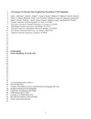
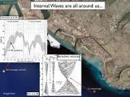
Figure 1: Vertical profiles of eddy 

kinetic energy ( 1 2 (u′2 + v ′2 )) for 

AUSSAF data compared with profiles 

from other sites in the ACC: 

southeast of New Zealand and 

Drake Passage (solid lines) and 

from western boundary current 

systems: Agulhas, Gulf Stream 

and Kuroshio Extension (dashed 

lines), from Phillips and Rintoul 

(2000). 

2 Spatial distribution of eddy mixing in the Southern Ocean 

In the absence of direct measurements of eddy mixing across the ACC, a number of studies 

have attempted to deduce horizontal and vertical distributions of eddy diffusivities. 

These studies have produced conflicting results, although, as we will explain below, they 

are consistent with different hypotheses for eddy diffusivity distributions. On the one 

hand, eddy diffusivities are hypothesized to be determined by eddy kinetic energy (EKE) 

(e.g. Keffer and Holloway, 1988; Stammer, 1998). A recent study found variations in eddy 

stirring and mixing rates using finite-time Lyapunov exponents to be closely related to 

variations in mesoscale activity, or √ EKE (Waugh and Abraham, 2008). Diffusivities inferred 

from Lagrangian floats are also often highly correlated with eddy kinetic energy 

(Krauss and Böning, 1987; Lumpkin et al., 2001; Zhurbas and Oh, 2003; Sallée et al., 2008), 

resulting in local maxima of eddy diffusivity in the core of the ACC (Sallée et al., 2008). 

On the other hand, strong currents can also act as mixing barriers (e.g. Bower et al., 1985), 

leading to small effective eddy diffusivities in the core of the ACC (e.g. Marshall et al., 

2006; Naveira Garabato et al., 2009). Naveira Garabato et al. (2009) employed mixing 

length arguments, and found that it is the spatial distribution of the eddy length scales, 

rather than the eddy velocities or EKE that determines the spatial distributions of the 

eddy diffusivities. At any given geographic location, the magnitude of the diffusivity 

depends on the relative importance of the strength of the mean flow and EKE respectively 

(Shuckburgh et al., 2008a,b). Griesel et al. (009b) reconciled some of the conflicting 

horizontal near-surface eddy diffusivity distributions by pointing out that dominant correlations 

of Lagrangian diffusivities with EKE may have been related to not using long 

enough time lags in the integral of the Lagrangian velocity autocovariance. However, the 

float deployments used by Griesel et al. (009b) were limited, both in number and spatial 

distribution, and did not resolve the ACC and the region north of the ACC sufficiently to 

D–3

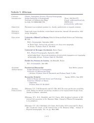
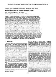
Figure 2: Depth dependence of alongstreamline 

averaged effective eddy diffusivities, 

estimated from tracers advected with 

the velocity of the Southern Ocean State 

estimate (SOSE) from Abernathy et al. 

(2008). 

distinguish regimes with strong and weak mean flow. 

There is also a lack of consensus on the depth dependence of the eddy diffusivities. 

Diffusivities are predicted to decrease with depth when the depth dependence is dominated 

by the decrease of eddy velocity or EKE with depth (see Figure 1). Such a decrease 

has been found by Ferreira et al. (2005); Eden (2006); Olbers and Visbeck (2005) 

and Griesel et al. (009a). Conversely, critical layer theory predicts that the diffusivity 

should have a maximum at the depth where the speed of the mean flow is comparable 

to the phase speed of Rossby waves (Green, 1970; Smith and Marshall, 2009). Indeed, 

enhanced diffusivities at depth have been diagnosed in eddying models of varying complexity 

by Cerovecki et al. (2009); Smith and Marshall (2009) and Abernathy et al. (2008) 

(see Figure 2), using the Nakamura (1996) method, and from flux/gradient relationships 

(Treguier, 1999; Smith and Marshall, 2009). Of the studies listed here, only our investigation 

(Griesel et al., 009b) used Lagrangian methods to investigate depth dependence. We 

found that depth invariant Lagrangian diffusivity in the core of the ACC jet arose from a 

combination of eddy velocities decreasing and Lagrangian eddy length scales increasing 

with depth. 

Even though eddy mixing can be diagnosed with different methods, the fundamental 

issue remains whether these eddy diffusion coefficients actually have sufficient skill to parameterize 

eddy transports in a downgradient parameterization. Challenges arise when 

attempting to correlate downgradient parameterizations with the eddy fluxes. One reason 

for low correlations of the eddy fluxes with their parameterizations and for unphysically 

large positive and negative values of the diffusivities is the presence of strong rotational 

components (Lau and Wallace, 1979; Marshall and Shutts, 1981, henceforth MS81). 

These rotational components of the eddy flux do not contribute to the local heat budget, 

since they transport as much heat into a region as out of it (Jayne and Marotzke, 2002). 

In previous work with POP Griesel et al. (009a) showed that the rotational component of 

the eddy heat flux dominates over all spatial scales. We also pointed out the challenges 

of finding eddy diffusion coefficients that are physically meaningful, smoothly varying 

and most importantly, that still capture most of the eddy flux in a downgradient parameterization. 

On the other hand, Griesel et al. (009b) have shown that the diffusive limit 

can be reached over lengthscales of 10 ◦ longitude with Lagrangian floats. One aim of 

D–4

the proposed work is to reconcile these two findings. Significantly more numerical float 

deployments than the O(100) deployments used in Griesel et al. (009b) are needed in order 

to sufficiently resolve spatial variability of Lagrangian diffusivities. Since Lagrangian 

floats are widely used and are an invaluable tool to assess eddy mixing from observations, 

it is important to be able to reconcile the previously reported estimates of eddy 

diffusivities that used different methods, as well as compare the Eulerian analysis with 

the Lagrangian eddy statistics. This will allow better interpretation of Lagrangian data 

that emerge from field programs. 

The Diapycnal and Isopycnal Mixing Experiment in the Southern Ocean (DIMES) will 

deploy a total of 180 RAFOS floats into the Southern Ocean. While DIMES will deliver a 

wealth of data on eddy mixing in the Southern Ocean, it is crucial to be able to interprete 

these properly. It is not feasible to deploy O(10,000) in the real ocean, and we will be able 

to develop the strategies for achieving robust results with the more limited data from the 

observational program. 

3 Objectives 

The first overarching goal of the proposed work is to characterize magnitudes and horizontal 

and vertical distributions of the Lagrangian eddy diffusivities in the Southern 

Ocean and to evaluate whether these can be reconciled with existing hypotheses. The 

hypotheses are that eddy diffusivities are to first order related to the spatial distributions 

of eddy kinetic energy, which would result in diffusivities being elevated at the surface 

and decreasing with depth in the core of the ACC. The alternative hypothesis is that eddy 

mixing is to first order determined by the relative strength of the mean flow and phase 

speed of Rossby waves, leading to the ACC jet acting as a mixing barrier at the surface, 

and diffusivities increasing in the core of the ACC jet. 

The second overarching goal is to investigate how well these diffusivities parameterize 

the integrated and local eddy tracer transports across the ACC. We propose to 

deploy a large number of numerical floats (O(10,000)) in POP, to quantify Lagrangian 

diffusivities and their spatial distributions, and to evaluate the relation of Eulerian eddy 

tracer fluxes and mean tracer gradients to assess the hypothesis that Lagrangian floats 

can be used to quantify eddy mixing and its spatial variation in the Southern Ocean. 

4 Approach and Methodology 

4.1 Objective 1: Characterizing the effects of eddies as a diffusive process 

using Lagrangian statistics 

4.1.1 Background 

Davis (1991) showed that the evolution of the mean tracer concentration in inhomogeneous 

flows with finite scale eddies depends only on the initial condition of the mean 

and source fields and the single particle statistics. The single particle Lagrangian diffu- 

D–5

sivity as a function of time lag is related to the Eulerian eddy fluxes and mean tracer 

gradients through the elaborated flux versus gradient law, 

〈u ′ i (x, t)Θ′ (x, t)〉 = lim τ−→∞ − 

∫ t 

0 

dτ∂ τ κ ij (x, τ)∂ xj Θ(x, t − τ) (1) 

Equation (1) specifies the flux of a (passive) tracer from the recent history of its mean 

concentration. The driving force for the eddy flux at time t is the sum of previous Θ gradients 

at times t − τ, weighted by the time derivative of κ at time range τ. κ will be defined 

below. This is an elaboration of the familiar advection-diffusion equation, where the elaboration 

reflects the finite scales of the eddies. If τ goes to infinity, or rather, is greater than 

some time T, that reflects the finite scales of the dispersing eddies, κ(x, t) approaches a 

constant value κ ∞ and the eddy flux is approximated by the typical advection-diffusion 

equation, 

〈u ′ i (x, t)Θ′ (x, t)〉 = −κ ∞ ij (x)∂ x j 

Θ(x, t) (2) 

The diffusivity κ ∞ is determined by the integral of the Lagrangian autocovariance 

function: 

κ ij (x, τ) = 

∫ 0 

−τ 

d ˜τ〈u ′ i (t 0|x, t 0 ) u ′ j (t 0 + ˜τ|x, t 0 )〉 L , (3) 

κ ∞ ij = lim τ−→∞ κ ij (x, τ), (4) 

where u ′ i (t 0 + τ|x, t 0 ) denotes the residual velocity of a particle at time t 0 + τ passing 

through x at time t 0 . For stationary and homogeneous statistics, the diffusivity is equal to 

half the time rate of change of the dispersion 〈d ′2 〉 

κ ij (x, τ) = 1 2 d t〈d ′ i (τ|x, t 0)d ′ j (τ|x, t 0)〉 L , (5) 

where d ′ (τ|x, t 0 ) is the displacement at time τ from its starting position, with the mean 

displacement removed. There are a number of challenges when computing Lagrangian 

diffusivities from eddying models, or oceanic data. To isolate the eddy velocities from the 

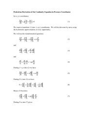
float velocities, a mean needs to be subtracted. As Figure 3a shows, the time-averaged Eulerian 

mean velocities are highly inhomogeneous in space. As shown by Oh et al. (2000), 

in a shear flow the along-stream diffusivity is affected by the shear dispersion. Therefore, 

if we remove a spatially-uniform average from each float velocity, we are left with a residual 

due to the mean shear that will imply dispersion and may dominate the diffusivity 

estimate (Bauer et al., 1998). Griesel et al. (009b) achieved good convergence properties 

of the Lagrangian diffusivities when they subtracted this Eulerian mean, thereby minimizing 

the influence of shear dispersion (Figure 3b,c). In an ocean with inhomogeneous, 

strong mean flows and with an eddy field of varying horizontal scale, the challenge is to 

find the asymptotic behavior of the velocity autocorrelation, which requires sufficiently 

long time lags (e.g. Bauer et al., 1998; Veneziani et al., 2004; Davis, 2005). The challenge 

arises because of the presence of strong rotational components in the eddy field, showing 

up in vortices or meanders of the Lagrangian trajectories that lead to oscillations in the autocovariances 

(Figure 4) as discussed by Berloff and McWilliams (2002a,b) and Veneziani 

D–6

a) 

⊥ dispersion (km 2 ) 

2 x 1011 

b) ⊥ 300m 

1 

0 

0 250 500 750 1000 

time lag (days) 

|| dispersion (km 2 ) 

3 x 1012 c) || 300m 

2 

1 

0 

0 250 500 750 1000 

time lag (days) 

Figure 3: a) Trajectories of 160 floats deployed at a depth of 300 m around latitude 60 ◦ S and 

longitude 180 ◦ W in one-quarter degree initial spacing from Griesel et al. (009b) after they have 

travelled for 1045 days (about 3 years). In color is the magnitude of the Eulerian 1998-1999 mean 

velocity interpolated to each float point. Lower panels show the corresponding long-time (1045 

days) mean square displacement for these trajectories in the cross-stream (b) and along-stream 

directions (c). The dispersion was calculated after subtraction of the spatially highly non-uniform 

Eulerian mean velocity in (a) from every float velocity. Shaded are 2*standard deviations from 

bootstrapping by subsampling the floats for each deployment with replacement. The dispersion 

is well approximated by the constant diffusivity at a time lag of 100 days (solid lines in a and b, 

where the dashed lines are the 95% confidence intervals). 

et al. (2005). Questions remain as to whether this is a transient behavior, or whether the 

diffusive limit can still be reached after long enough times lags (see Figure 3b,c), as suggested 

by Griesel et al. (009b). 

The Lagrangian diffusivity of Taylor can be expressed as the product of the eddy kinetic 

energy and an eddy decorrelation time scale T e , or, alternatively, with an eddy length 

scale L e = √ (EKE)T e . This eddy length scale can be interpreted as the mean displacement 

induced by an eddy. It is unclear how this eddy length scale is related to the typical 

eddy mixing length of for example Armi and Stommel (1983). Ferrari and Nikurashin 

(2009) and Naveira Garabato et al. (2009) hypothesize that the true mixing length of eddies 

is proportional to the Lagrangian eddy length scale divided by 1 + (U m − c) 2 , where 

U m is the strength of the mean flow and c is the phase speed of Rossby waves. In that 

sense, mixing length itself is dependent on eddy kinetic energy, and the eddy mixing 

length equals the Taylor eddy length scale, but reduced by the strength of the mean flow. 

This is in contrast to the assumption that in the presence of a mean flow the Taylor diffusivity 

by itself, as refined by Davis (1987, 1991), is able to quantify eddy mixing. 

D–7

cross−stream direction 

latitude 

300 

200 

100 

0 

−100 

−52 

−54 

−56 

−58 

−60 

along−stream direction 

−62 

180 190 200 210 220 

longitude 

3000 

a) b) 

c) 

κ m 2 s −1 ) 

κ (m 2 s −1 ) 

2000 

1000 

0 

−1000 

3000 

2000 

1000 

10 20 30 

tlag (days) 

d) 

0 

0 20 40 60 80 

tlag (days) 

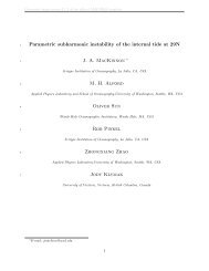
Figure 4: Circling and meandering trajectories 

(a) do not lead to any net cross-stream 

dispersion and the diffusivity as a function 

of time lag oscillates before it converges to 

the correct value of zero diffusivity (b). Real 

POP trajectories from Griesel et al. (009b) (c) 

show this oscillating behavior (d). Enough 

float trajectories such that the oscillations 

may cancel each other are needed as well as 

a long enough time lag to reach κ ∞ 

4.1.2 Float Deployments in POP 

The Los Alamos National Laboratory (LANL) Parallel Ocean Program (POP) has been 

configured on a 0.1 ◦ , 42-level global tripole grid, which is Mercator south of 28.5 ◦ N (Maltrud 

et al., 2008). The POP model has one of the highest horizontal resolutions used 

in global ocean modeling applications, leading to horizontal resolutions between 4 and 

9 km for the Southern Ocean. POP is eddy resolving in the sense that between about 

50 ◦ S and 50 ◦ N it resolves the first baroclinic Rossby radius, which is smaller than typical 

eddy length scales (Smith et al., 2000). To date the simulation has been run for 100 years 

and is forced with the monthly normal year atmospheric fluxes constructed by Large and 

Yeager (2004) for the Common Ocean-Ice Reference Experiments (CORE). Normal year 

forcing consists of single annual cycles of all atmospheric data needed to force an ocean 

model and is representative of climatological conditions over 43 years of interannually 

varying atmospheric state. It has been constructed to retain synoptic variability (i.e. atmospheric 

storms) with a seamless transition from 31 December to 1 January (Large and 

Yeager, 2004). The forcing uses the National Center for Environmental Prediction/ National 

Center for Atmospheric Research (NCEP/NCAR) reanalysis corrected with scatterometer 

data. A marked improvement was seen in the pathways of the Agulhas eddies, 

relative to the global 0.1 ◦ , 40-level standard z-level dipole simulation of Maltrud and Mc- 

Clean (2005). Here we propose to conduct a 5-10 year global tripole 0.1 ◦ POP simulation 

forced with interannually-varying synoptic CORE forcing for the more recent years 1997- 

2007 initialized from this spun-up ocean state. The exact duration of the run will depend 

on the throughput of the NSF Terascale high performance computing platforms available 

to us. We will, however, be able to archive 2-3 years of daily state variables and flux terms, 

and otherwise monthly means. 

To analyze Lagrangian motions, it is crucial that we are able to advect the POP floats 

as part of the model runs, using the time-varying three-dimensional velocity field. The 

position of the floats will be evaluated with a fourth-order Runge Kutta scheme at every 

model time step of 6 minutes. This is clearly an advantage over previous studies that 

used multiple-day averages of velocities to advect floats. As shown by (Griesel et al., 

D–8

009b), floats advected by the three-dimensional model field stay on isopycnal surfaces 

reasonably well, at least away from the oceanic surface and mixed layers. However, small 

deviations from isopycnals are evidence of small diapycnal mixing rates that can be crucial 

for Southern Ocean dynamics. Since there is great interest in understanding how 

three-dimensional motions may differ from isopycnal motions, we will also explore ways 

to correct the motion of the floats to force them to stay on an isopycnal. Additionally, 

there is the potential to investigate sensitivities of float trajectories to different advection 

schemes as well as model parameters. 

We propose to deploy a total of O(10,000) numerical floats in the following ways: 

(1) The depth dependence and horizontal variability of Lagrangian diffusivities has been 

investigated by Griesel et al. (009b), but spatial coverage of the floats was limited to the 

area within the ACC, and due to the limited number of floats, bins with significant realizations 

were sparse. To improve upon the numerical float deployments in POP, to 

achieve more spatial coverage within the ACC and also to cover the area north of the 

ACC, we propose to deploy floats at 4 different longitudes with a quarter degree initial 

spacing, and at latitudes corresponding to south of the Polar Frontal Zone, between the 

Polar Frontal Zone and Subantractic Front, and north of the Subantarctic Front. ”Point” 

deployments in this way will make it possible to track the spreading of a group of floats 

along one specific isopycnal interval. The mean position of the fronts will be estimated 

with time mean barotropic streamlines from the model. To sample with depth, the floats 

will be deployed at 4 different depth levels. 

(2) One deployment will be configured to match that of the DIMES experimental deployment 

scheme (around 105 ◦ W, 55 ◦ -60 ◦ S, and at two different depth levels, or isopycnal 

surfaces), to determine how well the limited number of floats deployed as part of DIMES 

can reproduce the magnitude and spatial variability of the extended deployments, and to 

help improve analysis methods for the real floats. 

(3) To assess sampling biases we will deploy the same number of floats as in (1) but distributed 

horizontally and vertically uniformly over the whole Southern Ocean. One of the 

main questions is whether Lagrangian statistics provide sufficient information to quantify 

possible mixing barriers at fronts, and whether Lagrangian statistics will be similar 

in this respect with uniform deployment as compared to when patches of floats are deployed 

in between the fronts as in (1) and (2). We will also address the question whether 

analysis in isopycnal space leads to similar conclusions compared to a situation in which 

the spreading of the floats is quantified with respect to depth interval. 

4.1.3 Analysis 

The goal of the proposed work is to infer robust Lagrangian diffusivities and spatial variation. 

We will use analysis scripts developed by Griesel et al. (009b) who have undertaken 

detailed sensitivity analysis. We will address the following questions: 

D–9

What are the characteristics of the Lagrangian trajectories in the Southern Ocean of 

POP relative to the mean streamlines? Bower and Rossby (1989) found that floats left 

the Gulf Stream much earlier at a depth of about 1000 m than closer to the surface, which 

could be an indication of enhanced eddy mixing at depth in the core of the Gulf Stream 

(see also Bower et al., 1985). However, deep floats were associated with little change 

in potential vorticity (PV) along their tracks, and therefore deep cross-stream exchange 

was not associated with cross-PV exchange (Bower, 1993). Several studies have examined 

mechanisms to explain how cross-stream exchange of fluid parcels is related to the 

occurence of meanders in jets (e.g. Bower, 1991; Dutkiewicz et al., 1993; Dutkiewicz and 

Paldor, 1994). Since we will archive the four-dimensional Eulerian POP fields, we will 

evaluate how cross-frontal exchanges are related to the meander time and space scale, to 

the definition of mean streamlines, and to the PV gradients. We will examine the individual 

pathways of the floats, and assess how quickly and where floats escape from the ACC 

and cross the Subantarctic Front. We will evaluate the length of time that floats remain 

within certain dynamical regimes, characterized for example by pressure or speed. These 

analyses will provide insights into where property exchanges occur and provide a basis 

for the following Lagrangian diffusivity and dispersion evaluation. 

Why and when is the diffusive limit reached? Our previous POP float results in the 

ACC have demonstrated the need to subtract spatially varying mean flows and the use 

of long enough time lags in the integral of the velocity autocovariance (Griesel et al., 

009b). One hypothesis is that with a large enough number of floats the oscillations in 

the diffusivity as a function of time lag (Figure 4) arising from rotational components 

will cancel each other, and the correct diffusive limit can be reached. On the other hand 

Griesel et al. (009a) have concluded that in the case of the Eulerian eddy heat fluxes, the 

rotational component is not reduced even if the fluxes are averaged over scales much 

larger than the eddy scales. The analysis of Griesel et al. (009b) also showed that upper 

ocean trajectories showed more meandering and looping behavior than trajectories from 

deeper isopycnal layers. This might be an indication of floats getting locked in with the 

mean flow meanders in the upper ocean leading to reduced eddy length scales. We will 

analyze in detail the sensitivities of κ ∞ from equation (4) to the definition of mean streamlines, 

the subtraction of different means, the number of floats used, the length of the time 

lag, and bin sizes. We will evaluate the number of looping and non-looping trajectories 

for different depth levels and within and outside the ACC and whether the diffusivity 

converges to the same limit if more and more trajectories are used. We will concentrate 

on the symmetric components of the diffusivity tensor from equation (4) that represent 

irreversible mixing processes but will also compare them to the antisymmetric parts. 

What are the robust horizontal and vertical distributions of the Lagrangian eddy diffusivities? 

With the proposed POP float deployments we will be able to sample regions 

both north and south of the Subantarctic Front. We will investigate the hypothesis that 

eddy mixing is suppressed in the core of the ACC whereas it is not supressed in areas 

where the strength of the mean flow is comparable to the phase speed of Rossby waves. 

Results will be compared to recent estimates from Marshall et al. (2006); Abernathy et al. 

(2008) and Naveira Garabato et al. (2009) who use different measures for the effective dif- 

D–10

Figure 5: Eddy temperature fluxes v ′ T ′ (a), mean temperature 

) 

gradients ∂ y T (b), the horizontal 

divergence of the eddy temperature flux ∇ h · 

(u ′ h T′ (c) and the Laplacian of mean temperature 

∇ 2 T (d) at a depth of 300 m in 1/10 ◦ POP for a region in the Agulhas Retroflection (see Griesel 

et al. (009a)). 

fusivity. According to Ferrari and Nikurashin (2009) and Naveira Garabato et al. (2009) 

the Taylor diffusivity may not be able to accurately capture the reduced mixing where the 

mean flow is strong. Here we will investigate the ability of Lagrangian statistics to detect 

mixing barriers. This will be achieved by correlating the strength of the mean flow and 

the size of the PV gradients with the Lagrangian diffusivities. 

4.2 Objective 2: How well do Lagrangian diffusivities parameterize 

Eulerian eddy tracer transports and their spatio-temporal distributions 

across the ACC? 

4.2.1 Background 

Davis (1987, 1991) developed the theoretical underpinning, in which way the single particle 

Lagrangian diffusivity as a function of time lag is related to the Eulerian eddy fluxes 

and mean tracer gradients (see equations 1-2). The term that actually enters the tracer 

balance equation is the divergence of the eddy tracer flux 

( 

) 

∇ · 〈u i ′ (x, t)Θ′ (x, t)〉 = ∇ · −κij ∞ (x)∂ x j 

Θ(x, t) 

(6) 

Challenges arise in relating the eddy tracer fluxes from the left-hand-sides of equations 

(2) and (6) with the mean tracer gradients from the right-hand-sides of equations (2) and 

(6). Eulerian eddy fluxes (Figure 5a) and the divergence of the eddy fluxes (Figure 5b), 

are locally not correlated with their respective parameterizations (Figure 5c,d). Accordingly, 

eddy diffusivities as calculated from the ratio of flux and mean tracer gradient or 

D–11

FT(curl)/[FT(div)+FT(curl)] 

1 

0.98 

0.96 

0.94 

5 m 

0.92 318m 

918m 

0.9 

0.001 0.01 0.1 1 

k [cycles/degree longitude] 

x 

10 

Figure 6: A comparison of rotational and divergent 

parts of the eddy heat flux in the ACC 

in POP as a function of wavenumber and 

for three different depth levels in the ACC. 

Shown is the spectrum of the curl of the horizontal 

eddy heat transport, normalized by the 

sum of the spectra of the curl and the divergence 

of the horizontal eddy heat transport 

PSD(∂ x v ′ T ′ −∂ y u ′ T ′ ) 

(PSD(∂ x u ′ T ′ +∂ y v ′ T ′ )+PSD(∂ x v ′ T ′ −∂ y u ′ T ′ )) , where 

PSD is the power spectral density. 

divergence of flux and divergence of mean tracer gradient, are extremely noisy with extremely 

high spatial variability and are not usable in climate models (Rix and Willebrand, 

1996; Roberts and Marshall, 2000; Nakamura and Chao, 2000; Eden et al., 2007a,b). One 

reason for low correlations of the eddy fluxes with their parameterizations and for unphysically 

large positive and negative values of the diffusivities is the presence of strong 

rotational components. However, it is clear that eddy fluxes systematically do affect the 

larger-scale, time-mean state. Griesel et al. (009a) investigated whether averaging over 

scales larger than the eddy scales will make the POP eddy heat fluxes more parameterizable 

as downgradient diffusion and concluded that the rotational part of the eddy fluxes 

as measured by the curl always dominates over the divergent part as measured by the divergence 

(Figure 6), no matter how much one averages. Rotational and divergent fluxes 

can be separated using a Helmholtz decomposition (e.g. Lau and Wallace, 1979; Roberts 

and Marshall, 2000; Drijfhout and Hazeleger, 2001; Jayne and Marotzke, 2002). However, 

the Helmholtz decomposition depends on the choice of boundary conditions and is therefore 

not unique (Fox-Kemper et al., 2003). It is also computationally fairly expensive. 

Alternatively, a rotational component can be identified by considering the eddy variance 

equation (MS81, Medvedev and Greatbatch, 2004; Eden et al., 2007a). The eddy 

tracer flux can be decomposed into advective, diffusive and rotational components. Adding 

or removing a rotational eddy flux does not change the mean tracer budget that involves 

the divergence of the eddy flux. To provide a closure, the rotational flux in Medvedev 

and Greatbatch (2004) is attributed to the component of the eddy variance flux that is parallel 

to mean tracer surfaces. The diffusive eddy tracer flux in turn is associated with the 

eddy variance flux that is normal to the mean tracer surfaces. Then, a diffusion coefficient 

can be divised that can serve as a diagnostic to the true irreversible eddy mixing taking 

place. For example, Eden (2006) calculated eddy diffusivitities by subtracting the MG 

rotational flux from the raw eddy fluxes and yielded a more physical representation of 

eddy diffusivities by reducing unphysical negative diffusivities. However, as was shown 

by Griesel et al. (009a), the isolation of meaningful rotational components based on the 

eddy variance equation is challenging. The reason is that the eddy advective terms in the 

eddy variance equation are so dominant that it is difficult to extract the part that balances 

the conversion term that is related to the irreversible mixing (Wilson and Williams, 2004; 

D–12

κ [m 2 /s] 

15000 

10000 

5000 

5 m 

318 m 

579 m 

918 m 

κ [m 2 /s] 

1500 

1000 

500 

5 m 

318 m 

579 m 

918 m 

0 

0.001 0.01 0.1 1 10 


x 

0 

0.001 0.01 0.1 1 10 


x 

Figure 7: Eulerian diffusivities as a function of zonal wavenumber (or averaging length scale) 

from Griesel et al. (009a) for the core of the ACC. Left: Case FG, which refers to diffusivities as 

calculated from the raw fluxes and mean temperature gradients. Right: Case DL, which refers to 

diffusivities as calculated from the divergence of the eddy fluxes and the divergence of the mean 

gradients. Colors represent different depth levels. Case F quasi diffusivities are much larger and 

show more wavenumber dependence than Case DL diffusivities. A general decrease with depth is 

apparent in both. 

Depth [m] 

0 

500 

1000 

1500 

2000 

2500 

κ ⊥ 

0 1000 2000 3000 

Figure 8: Lagrangian cross-stream diffusivities 

as a function of depth interval. Lines 

are along-streamline averages as a function of 

mean depth intervals 5 - 500 m, 500 - 1000 m, 

1000 - 1500 m, 1500 - 2500 m over three 

streamline intervals: south of Polar Front 

(red), around Polar Front (blue), north of Subantarctic 

Front (green), from South to North). 

Cerovecki et al., 2009; Griesel et al., 009a). These triple correlation terms need to be diagnosed 

with sufficient numerical accuracy. This means that having high qualilty data to 

ensure conservative discretization of the eddy variance equation by taking into account 

triple correlation terms is essential. With POP, we will be able to implement diagnostics 

of the eddy variance equation and rotational fluxes in a conservative manner online. We 

will assess whether diffusivity estimates are indeed more physically plausible when rotational 

fluxes based on the eddy variance equation are subtracted from the raw eddy 

fluxes. The ultimate goal is to come up with a set of Eulerian diffusivities, that we will be 

able to compare to the Lagrangian diffusivities in a consistent way. 

Eulerian eddy diffusivities decrease with depth in Griesel et al. (009a) (Figure 7), 

whereas the Lagrangian diffusivities are depth invariant in the core of the ACC (Figure 

8). The magnitudes of the Lagrangian diffusivities also differ. Eulerian quasi diffusivities, 

calculated from the ratio of eddy tracer fluxes and mean gradients, tend to be an order 

of magnitude higher than the Lagrangian ones. Eulerian diffusivities calculated from the 

ratio of the divergence of the eddy flux and the divergence of the mean gradients, tend 

to be about a factor of two smaller than the Lagrangian ones. We plan to explore this discrepancy 

which we suspect might be due to different axes orientation and differences in 

the role of the rotational parts. Another way of understanding the relationship between 

D–13

Eulerian and Lagrangian diagnostics is to assess whether the Eulerian and Lagrangian 

eddy scales are related (Middleton, 1985). This will enable us to infer whether the Lagrangian 

sampling is in the fixed-float or frozen-field regime (see Lumpkin et al., 2001). 

As a float passes through an eddy field, it mixes the field’s spatial and temporal variability 

in its time series of displacement. The resulting relationship between the Lagrangian time 

scale T L and the Eulerian time scale T E was quantified by Middleton (1985) for an idealized 

eddy field. Corrsin’s conjecture expresses the idea that while floats experience both 

temporal and spatial decay of the autocorrelation, the Eulerian diffusivities only observe 

the temporal decay, leading to Lagrangian eddy scales that are smaller than the Eulerian. 

4.2.2 Analysis 

The comparison and synthesis of the Lagrangian and Eulerian analyses will be twofold: 

(1) We will assess whether the estimated Lagrangian and Eulerian diffusivities have similar 

magnitudes and spatial distributions. This comparison will be carried out using both 

integrated and more local eddy tracer transports, and will involve evaluation of the elaborated 

flux versus gradient law (equation 1). (2) We will compare the different measures 

for eddy scales and assess how eddy scales and eddy diffusivities may be parameterized 

by large-scale quantities. We ask the following questions: 

How do Eulerian and Lagrangian diffusivities compare? We will first characterize the 

Eulerian eddy transports. We will assess the zonally and along-streamline averaged eddy 

tracer transports for different tracers (temperature, salinity, PV and a passive tracer), and 

their horizontal and vertical distribution. The raw eddy tracer fluxes will be compared 

to the divergence of the eddy tracer fluxes. We will then calculate eddy diffusivities from 

the ratio of the raw fluxes and mean tracer gradients, both averaged over the Lagrangian 

bins, and from the divergence of the eddy fluxes and parameterization. We will also 

compare these more local estimates to estimates arising when the eddy fluxes are averaged 

along circumpolar streamlines, thereby eliminating the rotational part. We ask how 

the depth dependence of these Eulerian diffusivities comes about from the depth dependence 

of the eddy fluxes and mean gradients, thereby considering that different tracers 

may exhibit different spatial distributions. Medvedev and Greatbatch (2004) and Eden 

et al. (2007a) have defined methods to compute the rotational components of fluxes by 

making use of a conservative discretization of the eddy variance budget. This requires a 

large number of terms, and we will therefore estimate the rotational fluxes as part of the 

POP model run rather than in the post analysis. We will then ask whether subtracting 

rotational components from the raw eddy fluxes produces eddy diffusivities with physically 

meaningful magnitudes and spatial patterns. These Eulerian diffusivities resulting 

from the subtraction of rotational parts will be compared to the diffusivities computed 

from the raw fluxes and gradients. Finally we will evaluate the extent to which the eddy 

flux in eq. (1) depends on the history of the mean field gradient. As noted by Davis (1987), 

when κ ∞ τ/L 2 c is not small, where κ ∞ is defined in equation (4, τ is the time lag and L c 

is a measure of the characteristic eddy length, there will be large fluctuations in the ratio 

of instantaneous flux and mean gradient. What are the consequences for the non-local 

definition of the Lagrangian diffusivity, and can it be reconciled with the fact that mean 

D–14

velocities and mean tracer gradient seem to be changing over scales that are comparable 

to the eddy scales? 

How do different definitions of eddy scales and their parameterization with large-scale 

quantities compare? We will compare the Lagrangian eddy scales as computed from the 

integral of the Lagrangian velocity autocovariance with the ones deduced from Eulerian 

time series at fixed points. Furthermore, we will calculate classical mixing lengths as defined 

by Armi and Stommel (1983) and used by e.g. Naveira Garabato et al. (2009). Can 

the classical mixing length be related to the Eulerian and Lagrangian eddy scales? And 

is there a difference in their spatial distributions? Finally, we will explore parameterizations 

of the eddy diffusivities themselves with the large-scale thermodynamic quantities 

that arise from theories of a baroclinically unstable flow field (Green, 1970; Stammer, 

1998). Central to these parameterizations is the measure of the growth rate of barolinic 

eddies 1/T bc = f / √ R i , where R i is the Richardson number obtained from the large-scale 

stratification and shear. The eddy diffusivity can be expressed in the general form as 

κ = αL bc T −1 

bc 

. We will test how well different formulations with different definitions of 

length scales L bc that have been proposed (Green, 1970; Stone, 1972; Held and Larichev, 

1996) compare to the Eulerian and Lagrangian eddy diffusivity estimates and their spatial 

distributions. 

4.3 Broader Impacts 

This project is motivated by the need to understand the role of ocean circulation in moderating 

climate, and by the need to improve climate models. The project will explore 

different ways to parameterize mixing coefficients, which will be testable in predictive 

climate models. A detailed assessment of Lagrangian methods and their relation to eddy 

fluxes and diffusivity estimates from other methods will benefit efforts to analyze data 

from floats deployed all over the ocean. In particular, the methods investigated in this 

study will contribute to the interpretation of in situ data returned by the 180 RAFOS 

floats that are being deployed as part of the Diapycnal and Isopycnal Mixing Experiment 

in the Southern Ocean (DIMES). Passive tracer fields, POP float trajectories and other POP 

output will be archived and made available to interested research groups. The proposed 

work will contribute to early career development of a postdoctoral researcher. 

D–15

References 

Abernathy, R., J. Marshall, E. Shuckburgh, and M. Mazloff, 2008: Studies of enhanced 

isopycnal mixing at deep critical levels in the Southern Ocean. J. Phys. Oceanogr., to be 

submitted. 

Armi, L. and H. Stommel, 1983: Four views of a portion of the north atlantic subtropical 

gyre. J. Phys. Oceanogr., 13, 828 – 857. 

Bauer, S., M. S. Swenson, A. Griffa, A. J. Mariano, and K. Owens, 1998: Eddy-mean flow 

decomposition and eddy-diffusivity estimates in the tropical Pacific Ocean. 1. Methodology. 

J. Geophys. Res., 103 (C13), 30,855 – 30,871. 

Berloff, P. S. and J. C. McWilliams, 2002a: Material transport in Oceanic gyres. Part I: 

Phenomenology. J. Phys. Oceanogr., 32, 764 – 796. 

———, 2002b: Material transport in Oceanic gyres. Part II: Hierarchy of stochastic models. 

J. Phys. Oceanogr., 32, 797 – 830. 

Böning, C. W., A. Dispert, M. Visbeck, S. R. Rintoul, and F. U. Schwarzkopf, 2008: The 

response of the Antarctic Circumpolar Current to recent climate change. Nature Geoscience, 

1, 864 – 869, doi: 10.1038/ngeo362. 

Bower, A. S., 1991: A simple kinematic mechanism for mixing fluid parcels across a meandering 

jet. J. Phys. Oceanogr., 21, 173 – 180. 

———, 1993: A closer look at particle exchange in the Gulf Stream. J. Phys. Oceanogr., 24, 

1399 – 1418. 

Bower, A. S. and H. T. Rossby, 1989: Evidence of cross-frontal exchange processes in the 

Gulg Stream based on isopycnal RAFOS float data. J. Phys. Oceanogr., 10, 1177 – 1190. 

Bower, A. S., H. T. Rossby, and J. L. Lillibridge, 1985: The Gulf Stream - Barrier or Blender? 


Bryden, H. L. and S. A. Cunningham, 2003: How wind-forcing and air-sea heat exchange 

determine the meridional temperature gradient and stratification for the Antarctic Circumpolar 

Current. J. Geophys. Res., 108 (C8), Art. No. 3275. 

Byrne, D. A. and J. L. McClean, 2008: Sea level anomaly signals in the Agulhas Current 

region. Geophys. Res. Lett., 35 (L13701), doi:10.1029/2008GL034 584. 

Cerovecki, I., R. A. Plumb, and W. Heres, 2009: Eddy transport and mixing in a wind and 

buoyancy driven jet on a sphere. J. Phys. Oceanogr., accepted. 

Danabasoglu, G. and J. Marshall, 2007: Effects of vertical variations of thickness diffusivity 

in an ocean general circulation model. Ocean Modelling, 18, 122 – 141. 

Davis, R., 1987: Modelling eddy transport of passive tracers. J. Mar. Res., 45, 635 – 666. 

E–1

———, 1991: Observing the general circulation with floats. Deep Sea Res., 38 ((Suppl. 1)), 

S531 – S571. 

———, 2005: Intermediate-depth circulation of the Iindian and South Pacific Oceans measured 

by autonomous floats. J. Phys. Oceanogr., 35, 683 – 707. 

Döös, K. and D. Webb, 1994: The Deacon cell and other meridional cells of the Southern 

Ocean. J. Phys. Oceanogr., 24, 429 – 442. 

Drijfhout, S. S. and W. Hazeleger, 2001: Eddy mixing of potential vorticity versus thickness 

in an isopycnic ocean model. J. Phys. Oceanogr., 31 (2), 481 – 505. 

Dutkiewicz, S., A. Griffa, and D. B. Olson, 1993: Particle diffusion in a meandering jet. 

J. Geophys. Res., 98, 16,487 – 16,500. 

Dutkiewicz, S. and N. Paldor, 1994: A note on the mixing enhancement in a meandering 

jet due to the interaction with an eddy. J. Phys. Oceanogr., 24, 2,418 – 2,423. 

Eden, C., 2006: Thickness diffusivity in the Southern Ocean. Geophys. Res. Lett., 33, 

doi:10.1029/2006GL026 157. 

Eden, C., R. J. Greatbatch, and D. Olbers, 2007a: Interpreting eddy fluxes. 

J. Phys. Oceanogr., 37 (5), 1282 – 1296. 

Eden, C., R. J. Greatbatch, and J. Willebrand, 2007b: A diagnosis of thickness fluxes in an 

eddy-resolving model. J. Phys. Oceanogr., 37 (3), 727 – 742. 

Ferrari, R. and M. Nikurashin, 2009: Suppression of eddy mixing across jets in the southern 

ocean. J. Phys. Oceanogr., submitted. 

Ferreira, D., J. Marshall, and P. Heimbach, 2005: Estimating eddy stresses by fitting dynamics 

to observations using a residual-mean ocean circulation model and its adjoint. 


Fox-Kemper, B., R. Ferrari, and J. Pedlosky, 2003: On the indeterminacy of rotational and 

divergent eddy fluxes. J. Phys. Oceanogr., 33, 478 – 483. 

Gent, P. R. and J. C. McWilliams, 1990: Isopycnal mixing in ocean circulation models. 


Gille, S. T., 2002: Warming of the southern ocean since the 1950s,. Science, 295, 1275 – 1277. 

———, 2008: Decadal-scale temperature trends in the southern hemisphere ocean. 

J. Clim., 21 (18), 4749 – 4765. 

Gille, S. T., A. Lombrozo, J. Sprintall, G. Stephenson, and R. Scarlet, 2009: Anomalous 

spiking in spectra of XCTD temperature profiles. J. Atmos. Ocean. Tech., 26 (6), 1157– 

1164. 

E–2

Gille, S. T., K. Speer, J. R. Ledwell, and A. C. Naveira Garabato, 2007: Mixing and stirring 

in the Southern Ocean. EOS, 88 (39), 382 – 383. 

Green, J. S., 1970: Transfer properties of the large-scale eddies and the general circulation 

of the atmosphere. Quart. J. Roy. Meteor. Soc., 96, 157 – 185. 

Griesel, A., S. T. Gille, J. Sprintall, J. L. McClean, J. H. LaCasce, and M. E. Maltrud, 2009b: 

Isopycnal diffusivities in the Antarctic Circumpolar Current inferred from lagrangian 

floats in an eddying model. to be submitted to JGR. 

Griesel, A., S. T. Gille, J. Sprintall, J. L. McClean, and M. E. Maltrud, 2009a: Assessing eddy 

heat flux and its parameterization: A wavenumber perspective from a 1/10 ◦ ocean 

simulation. Ocean Modelling, doi:10.1016/j.ocemod.2009.05.004. 

Griesel, A. and M. A. Morales Maqueda, 2006: The relation of meridional pressure gradients 

to North Atlantic Deep Water volume transport in an Ocean General Circulation 

Model. Clim. Dyn., 26 (7-8), 781 – 799. 

Griffies, S. M., 1998: The Gent-McWilliams skew flux. J. Phys. Oceanogr., 28, 831 – 841. 

Hallberg, R. W. and A. Gnanadesikan, 2006: The role of eddies in determining the structure 

and response of the wind-driven Southern hemisphere overturning: Results from 

the Modelling Eddies in the Southern Ocean (MESO) project. J. Phys. Oceanogr., 36, 2232 

– 2252. 

Held, K. M. and V. D. Larichev, 1996: A scaling theory for horizontally homogeneous, 

baroclinically unstable flow on a beta plane. J. Atmos. Sci., 53, 946 – 952. 

Hogg, A. M., J. P. Meredith, J. R. Blundell, and C. Wilson, 2008: Eddy heat flux in the 

Southern Ocean: Response to variable wind forcing. J. Clim., 21 (4), 608 – 620. 

Jayne, S. R. and J. Marotzke, 2002: The oceanic eddy heat transport. J. Phys. Oceanogr., 32, 

3328 – 3345. 

Johnson, G. C. and H. L. Bryden, 1989: On the size of the Antarctic Circumpolar Current. 

Deep Sea Res., 36, 39 – 53. 

Kamenkovich, I. and E. Sarachik, 2004: Mechanisms controlling the sensitivity of the 

Atlantic thermohaline circulation to the parameterization of eddy transports in ocean 

GCMs. J. Phys. Oceanogr., 34, 1628. 

Karsten, R., H. Jones, and J. Marshall, 2002: The role of eddy transfer in setting the stratification 

and transport of a circumpolar current. J. Phys. Oceanogr., 32 (1), 39 – 54. 

Karsten, R. and J. Marshall, 2002: Constructing the residual circulation of the ACC from 

observations. J. Phys. Oceanogr., 32, 3315 – 3327. 

Keffer, T. and G. Holloway, 1988: Estimating Southern Ocean eddy flux of heat and salt 

from satellite altimetry. Nature, 332, 624 – 626. 

E–3

Krauss, W. and C. Böning, 1987: Lagrangian properties of eddy fields in the northern 

North Atlantic as deduced from satellite-tracked buoys. J. Mar. Res., 45, 259 – 291. 

LaCasce, J. H., 2008: Lagrangian statistics from oceanic and atmospheric observations. 

Transport and Mixing in Geophysical Flows, Weiss, J. B. and A. Provenzale, Eds., Springer. 

Lau, N. C. and J. M. Wallace, 1979: On the distribution of horizontal transports by transient 

eddies in the Northern Hemisphere wintertime circulation. J. Atmos. Sci., 36, 1844 

– 1861. 

Lumpkin, R., A.-M. Treguier, and K. Speer, 2001: Lagrangian eddy scales in the Northern 

Atlantic Ocean. J. Phys. Oceanogr., 32, 2425 – 2440. 

Maltrud, M. E., F. Bryan, M. Hecht, E. Hunke, D. Ivanova, J. L. McClean, and S. Peacock, 

2008: Global Ocean Modelline in the eddying regime using POP. CLIVAR Exchanges, 

13 (1), 5 – 8. 

Maltrud, M. E. and J. L. McClean, 2005: An eddy resolving global 1/10 o ocean simulation. 

Ocean Modelling, 8 (1-2), 31 – 54. 

Marshall, J., D. Olbers, H. Ross, and D. Wolf-Gladrow, 1993: Potential vorticity constraints 

on the dynamics and hydrography of the Southern Ocean. J. Phys. Oceanogr., 23, 456 – 

487. 

Marshall, J. and T. Radko, 2003: Residual mean solutions for the Antarctic Circumpolar 

Current and its associated overturning circulation. J. Phys. Oceanogr., 33 (11), 2341 – 

2354. 

Marshall, J., E. Shuckburgh, H. Jones, and C. Hill, 2006: Estimates and implications 

of surface eddy diffusivity in the Southern Ocean derived from tracer transport. 


Marshall, J. and G. Shutts, 1981: 


A note on rotational and divergent eddy fluxes. 

McClean, J. L., D. P. Ivanova, and J. Sprintall, 2005: Remote origins of interannual variability 

in the Indonesian Throughflow region from data and a global POP simulation. 

J. Geophys. Res., 110 (C10013), doi:10.1029/2004JC002 858. 

McClean, J. L., S. Jayne, M. E. Maltrud, and D. P. Ivanova, 2008: The fidelity of ocean 

models with explicit eddies. Eddy-Resolving Ocean Modelling, Hecht, M. and H. Hasumi, 

Eds., AGU Monograph Series, in press. 

McClean, J. L., M. L. Maltrud, and F. O. Bryan, 2006: Measures of the fidelity of eddying 

ocean models. Oceanography, 19 (1), 60 – 73. 

Medvedev, A. S. and R. J. Greatbatch, 2004: On advection and diffusion in the mesosphere 

and lower thermosphere: The role of rotational fluxes. J. Geophys. Res., 109, D07 104, 

doi:10.1029/2003JD003 931. 

E–4

Middleton, J., 1985: Drifter spectra and diffusivities. J. Mar. Res., 43, 37 – 55. 

Nakamura, M. and Y. Chao, 2000: On the eddy isopycnal thickness diffusivity of the 

Gent-McWilliams subgrid mixing parameterization. J. Clim., 13, 502 – 510. 

Nakamura, N., 1996: Two-dimensional mixing, edge formation, and permeability in area 

coordinates. J. Atmos. Sci., 53, 1524 – 1537. 

Naveira Garabato, A. C., R. Ferrari, and K. L. Polzin, 2009: Eddy-induced mixing in the 

Southern Ocean. submitted to. 

Oh, S. I., V. Zhurbas, and W. S. Park, 2000: Estimating horizontal diffusivity in the East 

Sea (Sea of Japan) and the northwest Pacific from satellite-tracked drifter data. J. Geophys. 

Res., 105, 6483 – 6492. 

Olbers, D. and M. Visbeck, 2005: A model of the zonally averaged stratification and overturning 

in the Southern Ocean. J. Phys. Oceanogr., 35, 1190 – 1205. 

Phillips, H. E. and S. R. Rintoul, 2000: Eddy variability and energetics from direct 

current measurements in the Antarctic Circumpolar Current south of Australia. 


Prasad, T. G. and J. L. McClean, 2004: Mechanisms for anomalous warming in the 

western Indian Ocean during Dipole Mode events. J. Geophys. Res., 109 (C02019), 

doi:10.1029/2003JC001 872. 

Rainville, L., S. R. Jayne, J. L. McClean, and M. E. Maltrud, 2007: Formation of Subtropical 

Mode Water in a high-resolution POP simulation of the Kuroshio extension region. 

Ocean Modelling, 17, 338 – 356. 

Rix, N. H. and J. Willebrand, 1996: Parameterization of mesoscale eddies as inferred from 

a high-resolution circulation model. J. Phys. Oceanogr., 26, 2281 – 2285. 

Roberts, M. J. and D. P. Marshall, 2000: On the validity of downgradient eddy closures in 

ocean models. J. Geophys. Res., 105 (C12), 28,613 – 28,627. 

Sallée, J. B., K. Speer, R. Morrow, and R. Lumpkin, 2008: An estimate of Lagrangian eddy 

statistics and diffusion in the mixed layer of the Southern Ocean. J. Mar. Res. 

Shuckburgh, E., H. Jones, J. Marshall, and C. Hill, 2008a: Quantifying the eddy diffusivity 

of the Southern Ocean I: temporal variability. J. Phys. Oceanogr., submitted. 

———, 2008b: Quantifying the eddy diffusivity of the Southern Ocean II: spatial variability 

and the role of the mean flow. J. Phys. Oceanogr., submitted. 

Smith, K. and J. Marshall, 2009: Evidence for deep eddy mixing in the Southern Ocean. 


Smith, R. D., M. E. Maltrud, F. O. Bryan, and M. W. Hecht, 2000: Numerical simulation of 

the North Atlantic Ocean at 1/10 o . J. Phys. Oceanogr., 20, 1532 – 1561. 

E–5

Speer, K., S. R. Rintoul, and B. M. Sloyan, 2000: The diabatic Deacon cell. J. Phys. Oceanogr., 

30, 3212 – 3222. 

Stammer, D., 1998: On eddy characteristics, eddy transports and mean flow properties. 


Stone, P. H., 1972: A simplified radiative-dynamical model for the static stability of rotating 

atmospheres. J. Atmos. Sci., 29, 405 – 418. 

Taylor, G. I., 1921: Diffusion by continuous movements. Proc. Roy. Soc. A, 64, 476 – 490. 

Tokmakian, R. and J. L. McClean, 2003: How realistic is the high frequency signal of a 

0.1 ◦ ocean model? J. Geophys. Res., 108 (C4), 3115, doi:10.1029/2002JC001 446. 

Treguier, A. M., 1999: Evaluating eddy mixing coefficients from eddy-resolving ocean 

models: A case study. J. Mar. Res., 57, 89 – 108. 

Treguier, A. M., M. H. England, S. R. Rintoul, G. Madec, J. L. Sommer, and J.-M. Molines, 

2007: Southern Ocean overturning across streamlines in an eddying simulation of the 

Antarctic Circumpolar Current. Ocean Sci., 3, 491 – 507. 

Veneziani, M., A. Griffa, Z. D. Garraffo, and E. P. Chassignet, 2005: Lagrangian spin parameter 

and coherent structures from trajectories released in a high-resolution ocean 

model. J. Mar. Res., 63, 753 – 788. 

Veneziani, M., A. Griffa, A. M. Reynolds, and A. J. Mariano, 2004: Oceanic turbulence and 

stochastic models from subsurface lagrangian data for the north-west atlantic ocean. 


Waugh, D. W. and E. R. Abraham, 2008: Stirring in the global surface ocean. Geophys. 

Res. Lett., 35, L20 605, doi:10.1029/2008GL035 526. 

Wilson, C. and R. G. Williams, 2004: Why are eddy fluxes of potential vorticity difficult to 

parameterize ? J. Phys. Oceanogr., 34, 142 – 155. 

Zhurbas, V. and S. I. Oh, 2003: Drifter-derived maps of lateral diffusivity in the Pacific and 

Atlantic Oceans in relation to surface circulation patterns. J. Geophys. Res., 109, C05 015. 

E–6

NSF proposal - Physical Oceanography Research Division

You also want an ePaper? Increase the reach of your titles

Delete template?

Save as template?