How to Kill a Black Swan Remy Briand and David Owyong ...
How to Kill a Black Swan Remy Briand and David Owyong ...
How to Kill a Black Swan Remy Briand and David Owyong ...

Create successful ePaper yourself
Turn your PDF publications into a flip-book with our unique Google optimized e-Paper software.
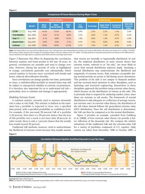
Figure 2<br />
Comparison Of Asset Returns During Major Crises<br />
Global Equities<br />
Global Bonds<br />
Month<br />
MSCI<br />
ACWI<br />
MSCI<br />
World (DM)<br />
MSCI<br />
EM<br />
U.S.<br />
T-Bills<br />
Sovereign<br />
High-Yield<br />
Premium<br />
Corporate<br />
Premium<br />
MSCI EM<br />
Currency<br />
Index<br />
LTCM Aug-1998 -14.2% -13.5% -29.3% 0.9% 2.5% -2.2% -1.5% -2.0%<br />
Tech Bubble Nov-2000 -6.2% -6.1% -8.8% 0.7% 2.0% -1.3% -0.7% -0.2%<br />
Sept 11 Sep-2001 -9.1% -8.8% -15.5% 1.0% 0.8% -1.4% -0.7% -2.0%<br />
Quant Crisis Aug-2007 -0.2% 0.0% -2.1% 0.7% 1.6% -0.8% -0.9% -0.8%<br />
Lehman Oct-2008 -19.8% -18.9% -27.4% 0.7% -1.9% -7.4% -6.3% -6.3%<br />
Note: The bond indices are sourced from Merrill Lynch, the T-bill data from the Federal Reserve <strong>and</strong> the rest are from MSCI Barra. All returns are based in U.S. dollars. The MSCI<br />
EM Currency Index measures the strength of emerging market currencies relative <strong>to</strong> the U.S. dollar. The high-yield <strong>and</strong> corporate bond premia are based on the differential in<br />
returns between the high-yield or corporate bond index <strong>and</strong> the sovereign bond index.<br />
Figure 3 illustrates this effect by displaying the correlations<br />
between equities <strong>and</strong> bond premia in the last 10 years. In<br />
general, correlations are unstable <strong>and</strong> tend <strong>to</strong> change over<br />
time. <strong>How</strong>ever, during the periods of crisis as highlighted<br />
in orange, correlations generally rose substantially, which<br />
caused equities <strong>to</strong> become more correlated with bonds <strong>and</strong><br />
hence reduced diversification benefits.<br />
Since correlations can change quickly over time, particularly<br />
in crises, a well-diversified portfolio in normal times may still<br />
be subject <strong>to</strong> unexpected volatility in extreme circumstances.<br />
It is therefore also important for us <strong>to</strong> underst<strong>and</strong> tail risk—<br />
particularly, how <strong>to</strong> estimate <strong>and</strong> manage it appropriately.<br />
Modeling Extreme Events<br />
A common statistic currently used <strong>to</strong> measure downside<br />
risk is value at risk (VaR). This statistic is defined as the maximum<br />
loss a portfolio is expected <strong>to</strong> incur over a specified<br />
time period, with a specified probability or confidence level.<br />
For example, if the one-week 99 percent VaR of a portfolio<br />
is 20 percent, then there is a 99 percent chance that the loss<br />
of this portfolio over a week is not more than 20 percent. In<br />
other words, there is only a 1 percent chance that the weekly<br />
loss would exceed 20 percent.<br />
Traditional VaR methods, however, tend <strong>to</strong> underestimate<br />
the likelihood of extreme events because they usually assume<br />
Figure 3<br />
that returns are normally or lognormally distributed. In reality,<br />
the empirical distribution of asset returns shows that<br />
extreme events, referred <strong>to</strong> as “fat tails,” are more likely <strong>to</strong><br />
occur than normal distribution patterns imply. Assuming a<br />
normal distribution may underestimate the likelihood <strong>and</strong><br />
magnitude of extreme losses. Risk estimates acceptable during<br />
normal periods are prone <strong>to</strong> fail during severe downturns.<br />
This problem of fat tails is not unique <strong>to</strong> financial markets<br />
<strong>and</strong> has received much attention in other disciplines, such as<br />
hydrology <strong>and</strong> structural engineering. Researchers in these<br />
disciplines approach this problem using extreme value theory,<br />
which focuses on the distribution of returns at the tails. This<br />
is precisely what is required for analyzing market crises, since<br />
these are extreme or tail events. The framework of normal<br />
distribution is only adequate as a reflection of average returns,<br />
not extreme ones. In extreme value theory, the distribution of<br />
the tail values instead follows the generalized extreme value<br />
(GEV) distribution. Once the tail distribution is determined,<br />
the VaR can then be computed as in the normal distribution.<br />
Figure 4 provides an example, extended from Goldberg<br />
et al. [2008], of how extreme value theory can provide a better<br />
reflection of the downside risk. We compare the relative<br />
robustness of the traditional VaR <strong>and</strong> the extreme-value VaR<br />
for a variety of portfolios composed of U.S. equities. Daily<br />
returns are taken from December 1996 <strong>to</strong> Oc<strong>to</strong>ber 2007, a<br />
Tech Bubble<br />
Correlation Between Equities And Bond Spreads In Last Ten Years<br />
Sept. 11<br />
WorldCom<br />
Bull Market: Correlations fell<br />
in<strong>to</strong> negative terri<strong>to</strong>ry<br />
12/98 6/99 12/99 6/00 12/00 6/01 12/01 6/02 12/02 6/03 12/03 6/04 12/04 6/05 12/05 6/06 12/06 6/07 12/07 6/08 12/08<br />
Quant Crisis<br />
Lehman<br />
0.8<br />
0.6<br />
0.4<br />
0.2<br />
0.0<br />
–0.2<br />
–0.4<br />
–0.6<br />
■ MSCI ACWI vs. High Yield Bond Premium<br />
■ Emerging Market Equity Premium vs. High Yield Bond Premium<br />
■ MSCI ACWI vs. Corporate Bond Premium<br />
■ Emerging Market Equity Premium vs. Corporate Bond Premium<br />
Sources: MSCI Barra, Merrill Lynch<br />
Note: Correlations are monthly, computed using all daily returns within each month, <strong>and</strong> smoothed by using a six-month moving average.<br />
12<br />
July/August 2009