Entropy Inference and the James-Stein Estimator, with Application to ...

More documents

Recommendations

Info

HAUSSER AND STRIMMER While the multinomial model with Dirichlet prior is standard Bayesian folklore (Gelman et al., 2004), there is no general agreement regarding which assignment of a k is best as noninformative prior—see for instance the discussion in Tuyl et al. (2008) and Geisser (1984). But, as shown later in this article, choosing inappropriate a k can easily cause the resulting estimator to perform worse than the ML estimator, thereby defeating the originally intended purpose. 2.4 NSB Estimator The NSB approach (Nemenman et al., 2002) avoids overrelying on a particular choice of a k in the Bayes estimator by using a more refined prior. Specifically, a Dirichlet mixture prior with infinite number of components is employed, constructed such that the resulting prior over the entropy is uniform. While the NSB estimator is one of the best entropy estimators available at present in terms of statistical properties, using the Dirichlet mixture prior is computationally expensive and somewhat slow for practical applications. 2.5 Chao-Shen Estimator Another recently proposed estimator is due to Chao and Shen (2003). This approach applies the Horvitz-Thompson estimator (Horvitz and Thompson, 1952) in combination with the Good-Turing correction (Good, 1953; Orlitsky et al., 2003) of the empirical cell probabilities to the problem of entropy estimation. The Good-Turing-corrected frequency estimates are ˆθ GT k = (1 − m 1 ML )ˆθ k , n where m 1 is the number of singletons, that is, cells with y k = 1. Used jointly with the Horvitz- Thompson estimator this results in Ĥ CS = − p ∑ k=1 ˆθ GT k log ˆθ GT k (1 −(1 − ˆθ GT k ) n ) , an estimator with remarkably good statistical properties (Vu et al., 2007). 3. A James-Stein Shrinkage Estimator The contribution of this paper is to introduce an entropy estimator that employs James-Stein-type shrinkage at the level of cell frequencies. As we will show below, this leads to an entropy estimator that is highly effective, both in terms of statistical accuracy and computational complexity. James-Stein-type shrinkage is a simple analytic device to perform regularized high-dimensional inference. It is ideally suited for small-sample settings - the original estimator (James and Stein, 1961) considered sample size n = 1. A general recipe for constructing shrinkage estimators is given in Appendix A. In this section, we describe how this approach can be applied to the specific problem of estimating cell frequencies. James-Stein shrinkage is based on averaging two very different models: a high-dimensional model with low bias and high variance, and a lower dimensional model with larger bias but smaller variance. The intensity of the regularization is determined by the relative weighting of the two models. Here we consider the convex combination ˆθ Shrink k = λt k +(1 − λ)ˆθ ML k , (4) 1472
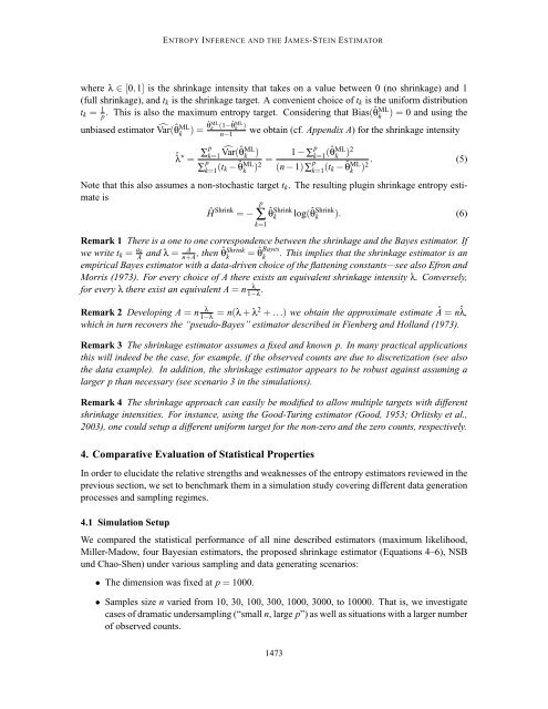
ENTROPY INFERENCE AND THE JAMES-STEIN ESTIMATOR where λ ∈ [0,1] is the shrinkage intensity that takes on a value between 0 (no shrinkage) and 1 (full shrinkage), and t k is the shrinkage target. A convenient choice of t k is the uniform distribution t k = 1 p . This is also the maximum entropy target. Considering that Bias(ˆθ ML k ) = 0 and using the unbiased estimator ̂Var(ˆθ ML k ) = ˆθ ML k (1−ˆθ ML k ) n−1 we obtain (cf. Appendix A) for the shrinkage intensity ˆλ ⋆ = ∑p k=1 ̂Var(ˆθ ML k ) ∑ p k=1 (t k − ˆθ ML k ) = 1 − ∑ p k=1 (ˆθ ML k ) 2 2 (n − 1)∑ p k=1 (t k − ˆθ ML (5) k ) 2. Note that this also assumes a non-stochastic target t k . The resulting plugin shrinkage entropy estimate is Ĥ Shrink = − p ∑ k=1 ˆθ Shrink k log(ˆθ Shrink k ). (6) Remark 1 There is a one to one correspondence between the shrinkage and the Bayes estimator. If we write t k = a k A and λ = A n+A , then ˆθ Shrink k = ˆθ Bayes k . This implies that the shrinkage estimator is an empirical Bayes estimator with a data-driven choice of the flattening constants—see also Efron and Morris (1973). For every choice of A there exists an equivalent shrinkage intensity λ. Conversely, for every λ there exist an equivalent A = n λ 1−λ . Remark 2 Developing A = n λ 1−λ = n(λ + λ2 + ...) we obtain the approximate estimate Â = nˆλ, which in turn recovers the “pseudo-Bayes” estimator described in Fienberg and Holland (1973). Remark 3 The shrinkage estimator assumes a fixed and known p. In many practical applications this will indeed be the case, for example, if the observed counts are due to discretization (see also the data example). In addition, the shrinkage estimator appears to be robust against assuming a larger p than necessary (see scenario 3 in the simulations). Remark 4 The shrinkage approach can easily be modified to allow multiple targets with different shrinkage intensities. For instance, using the Good-Turing estimator (Good, 1953; Orlitsky et al., 2003), one could setup a different uniform target for the non-zero and the zero counts, respectively. 4. Comparative Evaluation of Statistical Properties In order to elucidate the relative strengths and weaknesses of the entropy estimators reviewed in the previous section, we set to benchmark them in a simulation study covering different data generation processes and sampling regimes. 4.1 Simulation Setup We compared the statistical performance of all nine described estimators (maximum likelihood, Miller-Madow, four Bayesian estimators, the proposed shrinkage estimator (Equations 4–6), NSB und Chao-Shen) under various sampling and data generating scenarios: • The dimension was fixed at p = 1000. • Samples size n varied from 10, 30, 100, 300, 1000, 3000, to 10000. That is, we investigate cases of dramatic undersampling (“small n, large p”) as well as situations with a larger number of observed counts. 1473
Page 1 and 2: Journal of Machine Learning Researc
Page 3: ENTROPY INFERENCE AND THE JAMES-STE
Page 7 and 8: ENTROPY INFERENCE AND THE JAMES-STE

Entropy Inference and the James-Stein Estimator, with Application to ...

Create successful ePaper yourself

Delete template?

Save as template?