Entropy Inference and the James-Stein Estimator, with Application to ...
Entropy Inference and the James-Stein Estimator, with Application to ...
Entropy Inference and the James-Stein Estimator, with Application to ...

Create successful ePaper yourself
Turn your PDF publications into a flip-book with our unique Google optimized e-Paper software.
Journal of Machine Learning Research 10 (2009) 1469-1484 Submitted 10/08; Revised 4/09; Published 7/09<br />
<strong>Entropy</strong> <strong>Inference</strong> <strong>and</strong> <strong>the</strong> <strong>James</strong>-<strong>Stein</strong> <strong>Estima<strong>to</strong>r</strong>, <strong>with</strong> <strong>Application</strong> <strong>to</strong><br />
Nonlinear Gene Association Networks<br />
Jean Hausser<br />
Bioinformatics, Biozentrum<br />
University of Basel<br />
Klingelbergstr. 50/70<br />
CH-4056 Basel, Switzerl<strong>and</strong><br />
Korbinian Strimmer<br />
Institute for Medical Informatics, Statistics <strong>and</strong> Epidemiology<br />
University of Leipzig<br />
Härtelstr. 16–18<br />
D-04107 Leipzig, Germany<br />
JEAN.HAUSSER@UNIBAS.CH<br />
STRIMMER@UNI-LEIPZIG.DE<br />
Edi<strong>to</strong>r: Xiao<strong>to</strong>ng Shen<br />
Abstract<br />
We present a procedure for effective estimation of entropy <strong>and</strong> mutual information from smallsample<br />
data, <strong>and</strong> apply it <strong>to</strong> <strong>the</strong> problem of inferring high-dimensional gene association networks.<br />
Specifically, we develop a <strong>James</strong>-<strong>Stein</strong>-type shrinkage estima<strong>to</strong>r, resulting in a procedure that is<br />
highly efficient statistically as well as computationally. Despite its simplicity, we show that it outperforms<br />
eight o<strong>the</strong>r entropy estimation procedures across a diverse range of sampling scenarios<br />
<strong>and</strong> data-generating models, even in cases of severe undersampling. We illustrate <strong>the</strong> approach<br />
by analyzing E. coli gene expression data <strong>and</strong> computing an entropy-based gene-association network<br />
from gene expression data. A computer program is available that implements <strong>the</strong> proposed<br />
shrinkage estima<strong>to</strong>r.<br />
Keywords: entropy, shrinkage estimation, <strong>James</strong>-<strong>Stein</strong> estima<strong>to</strong>r, “small n, large p” setting, mutual<br />
information, gene association network<br />
1. Introduction<br />
<strong>Entropy</strong> is a fundamental quantity in statistics <strong>and</strong> machine learning. It has a large number of applications,<br />
for example in astronomy, cryp<strong>to</strong>graphy, signal processing, statistics, physics, image<br />
analysis neuroscience, network <strong>the</strong>ory, <strong>and</strong> bioinformatics—see, for example, Stinson (2006), Yeo<br />
<strong>and</strong> Burge (2004), MacKay (2003) <strong>and</strong> Strong et al. (1998). Here we focus on estimating entropy<br />
from small-sample data, <strong>with</strong> applications in genomics <strong>and</strong> gene network inference in mind (Margolin<br />
et al., 2006; Meyer et al., 2007).<br />
To define <strong>the</strong> Shannon entropy, consider a categorical r<strong>and</strong>om variable <strong>with</strong> alphabet size p <strong>and</strong><br />
associated cell probabilities θ 1 ,...,θ p <strong>with</strong> θ k > 0 <strong>and</strong> ∑ k θ k = 1. Throughout <strong>the</strong> article, we assume<br />
c○2009 Jean Hausser <strong>and</strong> Korbinian Strimmer.
HAUSSER AND STRIMMER<br />
that p is fixed <strong>and</strong> known. In this setting, <strong>the</strong> Shannon entropy in natural units is given by 1<br />
H = −<br />
p<br />
∑<br />
k=1<br />
θ k log(θ k ). (1)<br />
In practice, <strong>the</strong> underlying probability mass function are unknown, hence H <strong>and</strong> θ k need <strong>to</strong> be<br />
estimated from observed cell counts y k ≥ 0.<br />
A particularly simple <strong>and</strong> widely used estima<strong>to</strong>r of entropy is <strong>the</strong> maximum likelihood (ML)<br />
estima<strong>to</strong>r<br />
Ĥ ML = −<br />
p<br />
∑<br />
k=1<br />
constructed by plugging <strong>the</strong> ML frequency estimates<br />
ˆθ ML<br />
k log(ˆθ ML<br />
k )<br />
ˆθ ML<br />
k<br />
= y k<br />
n<br />
(2)<br />
in<strong>to</strong> Equation 1, <strong>with</strong> n = ∑ p k=1 y k being <strong>the</strong> <strong>to</strong>tal number of counts.<br />
In situations <strong>with</strong> n ≫ p, that is, when <strong>the</strong> dimension is low <strong>and</strong> when <strong>the</strong>re are many observation,<br />
it is easy <strong>to</strong> infer entropy reliably, <strong>and</strong> it is well-known that in this case <strong>the</strong> ML estima<strong>to</strong>r is<br />
optimal. However, in high-dimensional problems <strong>with</strong> n ≪ p it becomes extremely challenging <strong>to</strong><br />
estimate <strong>the</strong> entropy. Specifically, in <strong>the</strong> “small n, large p” regime <strong>the</strong> ML estima<strong>to</strong>r performs very<br />
poorly <strong>and</strong> severely underestimates <strong>the</strong> true entropy.<br />
While entropy estimation has a long his<strong>to</strong>ry tracing back <strong>to</strong> more than 50 years ago, it is only<br />
recently that <strong>the</strong> specific issues arising in high-dimensional, undersampled data sets have attracted<br />
attention. This has lead <strong>to</strong> two recent innovations, namely <strong>the</strong> NSB algorithm (Nemenman et al.,<br />
2002) <strong>and</strong> <strong>the</strong> Chao-Shen estima<strong>to</strong>r (Chao <strong>and</strong> Shen, 2003), both of which are now widely considered<br />
as benchmarks for <strong>the</strong> small-sample entropy estimation problem (Vu et al., 2007).<br />
Here, we introduce a novel <strong>and</strong> highly efficient small-sample entropy estima<strong>to</strong>r based on <strong>James</strong>-<br />
<strong>Stein</strong> shrinkage (Gruber, 1998). Our method is fully analytic <strong>and</strong> hence computationally inexpensive.<br />
Moreover, our procedure simultaneously provides estimates of <strong>the</strong> entropy <strong>and</strong> of <strong>the</strong> cell<br />
frequencies suitable for plugging in<strong>to</strong> <strong>the</strong> Shannon entropy formula (Equation 1). Thus, in comparison<br />
<strong>the</strong> estima<strong>to</strong>r we propose is simpler, very efficient, <strong>and</strong> at <strong>the</strong> same time more versatile than<br />
currently available entropy estima<strong>to</strong>rs.<br />
2. Conventional Methods for Estimating <strong>Entropy</strong><br />
<strong>Entropy</strong> estima<strong>to</strong>rs can be divided in<strong>to</strong> two groups: i) methods, that rely on estimates of cell frequencies,<br />
<strong>and</strong> ii) estima<strong>to</strong>rs, that directly infer entropy <strong>with</strong>out estimating a compatible set of θ k .<br />
Most methods discussed below fall in<strong>to</strong> <strong>the</strong> first group, except for <strong>the</strong> Miller-Madow <strong>and</strong> NSB<br />
approaches.<br />
1. In this paper we use <strong>the</strong> following conventions: log denotes <strong>the</strong> natural logarithm (not base 2 or base 10), <strong>and</strong> we<br />
define 0log0 = 0.<br />
1470
ENTROPY INFERENCE AND THE JAMES-STEIN ESTIMATOR<br />
2.1 Maximum Likelihood Estimate<br />
The connection between observed counts y k <strong>and</strong> frequencies θ k is given by <strong>the</strong> multinomial distribution<br />
p<br />
n!<br />
Prob(y 1 ,...,y p ;θ 1 ,...,θ p ) =<br />
∏ p k=1 y ∏ θ y k<br />
k<br />
k!<br />
. (3)<br />
Note that θ k > 0 because o<strong>the</strong>rwise <strong>the</strong> distribution is singular. In contrast, <strong>the</strong>re may be (<strong>and</strong><br />
often are) zero counts y k . The ML estima<strong>to</strong>r of θ k maximizes <strong>the</strong> right h<strong>and</strong> side of Equation 3 for<br />
fixed y k , leading <strong>to</strong> <strong>the</strong> observed frequencies ˆθ ML<br />
k<br />
= y k<br />
n<br />
<strong>with</strong> variances Var(ˆθ ML<br />
k<br />
) = 1 n θ k(1 − θ k ) <strong>and</strong><br />
Bias(ˆθ ML<br />
k<br />
) = 0 as E(ˆθ ML<br />
k<br />
) = θ k .<br />
2.2 Miller-Madow <strong>Estima<strong>to</strong>r</strong><br />
While ˆθ ML<br />
k<br />
is unbiased, <strong>the</strong> corresponding plugin entropy estima<strong>to</strong>r Ĥ ML is not. First order bias<br />
correction leads <strong>to</strong><br />
Ĥ MM = Ĥ ML + m >0 − 1<br />
,<br />
2n<br />
where m >0 is <strong>the</strong> number of cells <strong>with</strong> y k > 0. This is known as <strong>the</strong> Miller-Madow estima<strong>to</strong>r (Miller,<br />
1955).<br />
2.3 Bayesian <strong>Estima<strong>to</strong>r</strong>s<br />
Bayesian regularization of cell counts may lead <strong>to</strong> vast improvements over <strong>the</strong> ML estima<strong>to</strong>r (Agresti<br />
<strong>and</strong> Hitchcock, 2005). Using <strong>the</strong> Dirichlet distribution <strong>with</strong> parameters a 1 ,a 2 ,...,a p as prior, <strong>the</strong><br />
resulting posterior distribution is also Dirichlet <strong>with</strong> mean<br />
ˆθ Bayes<br />
k<br />
= y k + a k<br />
n+A ,<br />
where A = ∑ p k=1 a k. The flattening constants a k play <strong>the</strong> role of pseudo-counts (compare <strong>with</strong> Equation<br />
2), so that A may be interpreted as <strong>the</strong> a priori sample size.<br />
Some common choices for a k are listed in Table 1, along <strong>with</strong> references <strong>to</strong> <strong>the</strong> corresponding<br />
plugin entropy estima<strong>to</strong>rs,<br />
Ĥ Bayes = −<br />
p<br />
∑<br />
k=1<br />
ˆθ Bayes<br />
k<br />
log(ˆθ Bayes<br />
k<br />
).<br />
k=1<br />
a k Cell frequency prior <strong>Entropy</strong> estima<strong>to</strong>r<br />
0 no prior maximum likelihood<br />
1/2 Jeffreys prior (Jeffreys, 1946) Krichevsky <strong>and</strong> Trofimov (1981)<br />
1 Bayes-Laplace uniform prior Holste et al. (1998)<br />
1/p Perks prior (Perks, 1947) Schürmann <strong>and</strong> Grassberger (1996)<br />
√ n/p minimax prior (Trybula, 1958)<br />
Table 1: Common choices for <strong>the</strong> parameters of <strong>the</strong> Dirichlet prior in <strong>the</strong> Bayesian estima<strong>to</strong>rs of<br />
cell frequencies, <strong>and</strong> corresponding entropy estima<strong>to</strong>rs.<br />
1471
HAUSSER AND STRIMMER<br />
While <strong>the</strong> multinomial model <strong>with</strong> Dirichlet prior is st<strong>and</strong>ard Bayesian folklore (Gelman et al.,<br />
2004), <strong>the</strong>re is no general agreement regarding which assignment of a k is best as noninformative<br />
prior—see for instance <strong>the</strong> discussion in Tuyl et al. (2008) <strong>and</strong> Geisser (1984). But, as shown later<br />
in this article, choosing inappropriate a k can easily cause <strong>the</strong> resulting estima<strong>to</strong>r <strong>to</strong> perform worse<br />
than <strong>the</strong> ML estima<strong>to</strong>r, <strong>the</strong>reby defeating <strong>the</strong> originally intended purpose.<br />
2.4 NSB <strong>Estima<strong>to</strong>r</strong><br />
The NSB approach (Nemenman et al., 2002) avoids overrelying on a particular choice of a k in <strong>the</strong><br />
Bayes estima<strong>to</strong>r by using a more refined prior. Specifically, a Dirichlet mixture prior <strong>with</strong> infinite<br />
number of components is employed, constructed such that <strong>the</strong> resulting prior over <strong>the</strong> entropy is<br />
uniform. While <strong>the</strong> NSB estima<strong>to</strong>r is one of <strong>the</strong> best entropy estima<strong>to</strong>rs available at present in<br />
terms of statistical properties, using <strong>the</strong> Dirichlet mixture prior is computationally expensive <strong>and</strong><br />
somewhat slow for practical applications.<br />
2.5 Chao-Shen <strong>Estima<strong>to</strong>r</strong><br />
Ano<strong>the</strong>r recently proposed estima<strong>to</strong>r is due <strong>to</strong> Chao <strong>and</strong> Shen (2003). This approach applies <strong>the</strong><br />
Horvitz-Thompson estima<strong>to</strong>r (Horvitz <strong>and</strong> Thompson, 1952) in combination <strong>with</strong> <strong>the</strong> Good-Turing<br />
correction (Good, 1953; Orlitsky et al., 2003) of <strong>the</strong> empirical cell probabilities <strong>to</strong> <strong>the</strong> problem of<br />
entropy estimation. The Good-Turing-corrected frequency estimates are<br />
ˆθ GT<br />
k = (1 − m 1 ML<br />
)ˆθ k ,<br />
n<br />
where m 1 is <strong>the</strong> number of single<strong>to</strong>ns, that is, cells <strong>with</strong> y k = 1. Used jointly <strong>with</strong> <strong>the</strong> Horvitz-<br />
Thompson estima<strong>to</strong>r this results in<br />
Ĥ CS = −<br />
p<br />
∑<br />
k=1<br />
ˆθ GT<br />
k<br />
log ˆθ GT<br />
k<br />
(1 −(1 − ˆθ GT<br />
k<br />
) n ) ,<br />
an estima<strong>to</strong>r <strong>with</strong> remarkably good statistical properties (Vu et al., 2007).<br />
3. A <strong>James</strong>-<strong>Stein</strong> Shrinkage <strong>Estima<strong>to</strong>r</strong><br />
The contribution of this paper is <strong>to</strong> introduce an entropy estima<strong>to</strong>r that employs <strong>James</strong>-<strong>Stein</strong>-type<br />
shrinkage at <strong>the</strong> level of cell frequencies. As we will show below, this leads <strong>to</strong> an entropy estima<strong>to</strong>r<br />
that is highly effective, both in terms of statistical accuracy <strong>and</strong> computational complexity.<br />
<strong>James</strong>-<strong>Stein</strong>-type shrinkage is a simple analytic device <strong>to</strong> perform regularized high-dimensional<br />
inference. It is ideally suited for small-sample settings - <strong>the</strong> original estima<strong>to</strong>r (<strong>James</strong> <strong>and</strong> <strong>Stein</strong>,<br />
1961) considered sample size n = 1. A general recipe for constructing shrinkage estima<strong>to</strong>rs is given<br />
in Appendix A. In this section, we describe how this approach can be applied <strong>to</strong> <strong>the</strong> specific problem<br />
of estimating cell frequencies.<br />
<strong>James</strong>-<strong>Stein</strong> shrinkage is based on averaging two very different models: a high-dimensional<br />
model <strong>with</strong> low bias <strong>and</strong> high variance, <strong>and</strong> a lower dimensional model <strong>with</strong> larger bias but smaller<br />
variance. The intensity of <strong>the</strong> regularization is determined by <strong>the</strong> relative weighting of <strong>the</strong> two<br />
models. Here we consider <strong>the</strong> convex combination<br />
ˆθ Shrink<br />
k<br />
= λt k +(1 − λ)ˆθ ML<br />
k , (4)<br />
1472
ENTROPY INFERENCE AND THE JAMES-STEIN ESTIMATOR<br />
where λ ∈ [0,1] is <strong>the</strong> shrinkage intensity that takes on a value between 0 (no shrinkage) <strong>and</strong> 1<br />
(full shrinkage), <strong>and</strong> t k is <strong>the</strong> shrinkage target. A convenient choice of t k is <strong>the</strong> uniform distribution<br />
t k = 1 p<br />
. This is also <strong>the</strong> maximum entropy target. Considering that Bias(ˆθ<br />
ML<br />
k<br />
) = 0 <strong>and</strong> using <strong>the</strong><br />
unbiased estima<strong>to</strong>r ̂Var(ˆθ ML<br />
k<br />
) =<br />
ˆθ ML<br />
k<br />
(1−ˆθ ML<br />
k )<br />
n−1<br />
we obtain (cf. Appendix A) for <strong>the</strong> shrinkage intensity<br />
ˆλ ⋆ = ∑p k=1 ̂Var(ˆθ<br />
ML<br />
k<br />
)<br />
∑ p k=1 (t k − ˆθ ML<br />
k<br />
) = 1 − ∑ p k=1<br />
(ˆθ<br />
ML<br />
k<br />
) 2<br />
2 (n − 1)∑ p k=1 (t k − ˆθ ML<br />
(5)<br />
k<br />
) 2.<br />
Note that this also assumes a non-s<strong>to</strong>chastic target t k . The resulting plugin shrinkage entropy estimate<br />
is<br />
Ĥ Shrink = −<br />
p<br />
∑<br />
k=1<br />
ˆθ Shrink<br />
k log(ˆθ Shrink<br />
k ). (6)<br />
Remark 1 There is a one <strong>to</strong> one correspondence between <strong>the</strong> shrinkage <strong>and</strong> <strong>the</strong> Bayes estima<strong>to</strong>r. If<br />
we write t k = a k<br />
A <strong>and</strong> λ = A<br />
n+A , <strong>the</strong>n ˆθ Shrink<br />
k<br />
= ˆθ Bayes<br />
k<br />
. This implies that <strong>the</strong> shrinkage estima<strong>to</strong>r is an<br />
empirical Bayes estima<strong>to</strong>r <strong>with</strong> a data-driven choice of <strong>the</strong> flattening constants—see also Efron <strong>and</strong><br />
Morris (1973). For every choice of A <strong>the</strong>re exists an equivalent shrinkage intensity λ. Conversely,<br />
for every λ <strong>the</strong>re exist an equivalent A = n λ<br />
1−λ .<br />
Remark 2 Developing A = n λ<br />
1−λ = n(λ + λ2 + ...) we obtain <strong>the</strong> approximate estimate  = nˆλ,<br />
which in turn recovers <strong>the</strong> “pseudo-Bayes” estima<strong>to</strong>r described in Fienberg <strong>and</strong> Holl<strong>and</strong> (1973).<br />
Remark 3 The shrinkage estima<strong>to</strong>r assumes a fixed <strong>and</strong> known p. In many practical applications<br />
this will indeed be <strong>the</strong> case, for example, if <strong>the</strong> observed counts are due <strong>to</strong> discretization (see also<br />
<strong>the</strong> data example). In addition, <strong>the</strong> shrinkage estima<strong>to</strong>r appears <strong>to</strong> be robust against assuming a<br />
larger p than necessary (see scenario 3 in <strong>the</strong> simulations).<br />
Remark 4 The shrinkage approach can easily be modified <strong>to</strong> allow multiple targets <strong>with</strong> different<br />
shrinkage intensities. For instance, using <strong>the</strong> Good-Turing estima<strong>to</strong>r (Good, 1953; Orlitsky et al.,<br />
2003), one could setup a different uniform target for <strong>the</strong> non-zero <strong>and</strong> <strong>the</strong> zero counts, respectively.<br />
4. Comparative Evaluation of Statistical Properties<br />
In order <strong>to</strong> elucidate <strong>the</strong> relative strengths <strong>and</strong> weaknesses of <strong>the</strong> entropy estima<strong>to</strong>rs reviewed in <strong>the</strong><br />
previous section, we set <strong>to</strong> benchmark <strong>the</strong>m in a simulation study covering different data generation<br />
processes <strong>and</strong> sampling regimes.<br />
4.1 Simulation Setup<br />
We compared <strong>the</strong> statistical performance of all nine described estima<strong>to</strong>rs (maximum likelihood,<br />
Miller-Madow, four Bayesian estima<strong>to</strong>rs, <strong>the</strong> proposed shrinkage estima<strong>to</strong>r (Equations 4–6), NSB<br />
und Chao-Shen) under various sampling <strong>and</strong> data generating scenarios:<br />
• The dimension was fixed at p = 1000.<br />
• Samples size n varied from 10, 30, 100, 300, 1000, 3000, <strong>to</strong> 10000. That is, we investigate<br />
cases of dramatic undersampling (“small n, large p”) as well as situations <strong>with</strong> a larger number<br />
of observed counts.<br />
1473
HAUSSER AND STRIMMER<br />
The true cell probabilities θ 1 ,...,θ 1000 were assigned in four different fashions, corresponding <strong>to</strong><br />
rows 1-4 in Figure 1:<br />
1. Sparse <strong>and</strong> heterogeneous, following a Dirichlet distribution <strong>with</strong> parameter a = 0.0007,<br />
2. R<strong>and</strong>om <strong>and</strong> homogeneous, following a Dirichlet distribution <strong>with</strong> parameter a = 1,<br />
3. As in scenario 2, but <strong>with</strong> half of <strong>the</strong> cells containing structural zeros, <strong>and</strong><br />
4. Following a Zipf-type power law.<br />
For each sampling scenario <strong>and</strong> sample size, we conducted 1000 simulation runs. In each run, we<br />
generated a new set of true cell frequencies <strong>and</strong> subsequently sampled observed counts y k from <strong>the</strong><br />
corresponding multinomial distribution. The resulting counts y k were <strong>the</strong>n supplied <strong>to</strong> <strong>the</strong> various<br />
entropy <strong>and</strong> cell frequencies estima<strong>to</strong>rs <strong>and</strong> <strong>the</strong> squared error ∑ 1000<br />
i=k (θ k − ˆθ k ) 2 was computed. From<br />
<strong>the</strong> 1000 repetitions we estimated <strong>the</strong> mean squared error (MSE) of <strong>the</strong> cell frequencies by averaging<br />
over <strong>the</strong> individual squared errors (except for <strong>the</strong> NSB, Miller-Madow, <strong>and</strong> Chao-Shen estima<strong>to</strong>rs).<br />
Similarly, we computed estimates of MSE <strong>and</strong> bias of <strong>the</strong> inferred entropies.<br />
4.2 Summary of Results from Simulations<br />
Figure 1 displays <strong>the</strong> results of <strong>the</strong> simulation study, which can be summarized as follows:<br />
• Unsurprisingly, all estima<strong>to</strong>rs perform well when <strong>the</strong> sample size is large.<br />
• The maximum likelihood <strong>and</strong> Miller-Madow estima<strong>to</strong>rs perform worst, except for scenario 1.<br />
Note that <strong>the</strong>se estima<strong>to</strong>rs are inappropriate even for moderately large sample sizes. Fur<strong>the</strong>rmore,<br />
<strong>the</strong> bias correction of <strong>the</strong> Miller-Madow estima<strong>to</strong>r is not particularly effective.<br />
• The minimax <strong>and</strong> 1/p Bayesian estima<strong>to</strong>rs tend <strong>to</strong> perform slightly better than maximum<br />
likelihood, but not by much.<br />
• The Bayesian estima<strong>to</strong>rs <strong>with</strong> pseudocounts 1/2 <strong>and</strong> 1 perform very well even for small sample<br />
sizes in <strong>the</strong> scenarios 2 <strong>and</strong> 3. However, <strong>the</strong>y are less efficient in scenario 4, <strong>and</strong> completely<br />
fail in scenario 1.<br />
• Hence, <strong>the</strong> Bayesian estima<strong>to</strong>rs can perform better or worse than <strong>the</strong> ML estima<strong>to</strong>r, depending<br />
on <strong>the</strong> choice of <strong>the</strong> prior <strong>and</strong> on <strong>the</strong> sampling scenario.<br />
• The NSB, <strong>the</strong> Chao-Shen <strong>and</strong> <strong>the</strong> shrinkage estima<strong>to</strong>r all are statistically very efficient <strong>with</strong><br />
small MSEs in all four scenarios, regardless of sample size.<br />
• The NSB <strong>and</strong> Chao-Shen estima<strong>to</strong>rs are nearly unbiased in scenario 3.<br />
The three <strong>to</strong>p-performing estima<strong>to</strong>rs are <strong>the</strong> NSB, <strong>the</strong> Chao-Shen <strong>and</strong> <strong>the</strong> prosed shrinkage estima<strong>to</strong>r.<br />
When it comes <strong>to</strong> estimating <strong>the</strong> entropy, <strong>the</strong>se estima<strong>to</strong>rs can be considered identical for<br />
practical purposes. However, <strong>the</strong> shrinkage estima<strong>to</strong>r is <strong>the</strong> only one that simultaneously estimates<br />
cell frequencies suitable for use <strong>with</strong> <strong>the</strong> Shannon entropy formula (Equation 1), <strong>and</strong> it does so<br />
<strong>with</strong> high accuracy even for small samples. In comparison, <strong>the</strong> NSB estima<strong>to</strong>r is by far <strong>the</strong> slowest<br />
method: in our simulations, <strong>the</strong> shrinkage estima<strong>to</strong>r was faster by a fac<strong>to</strong>r of 1000.<br />
1474
ENTROPY INFERENCE AND THE JAMES-STEIN ESTIMATOR<br />
Probability density<br />
MSE cell frequencies<br />
MSE entropy<br />
Bias entropy<br />
probability<br />
0.0 0.2 0.4 0.6<br />
H = 1.11<br />
Dirichlet<br />
a=0.0007, p=1000<br />
estimated MSE<br />
0.0 0.2 0.4<br />
ML<br />
1/2<br />
1<br />
1/p<br />
minimax<br />
Shrink<br />
estimated MSE<br />
0 20 40 60 80<br />
Miller−Madow<br />
Chao−Shen<br />
NSB<br />
estimated Bias<br />
0 2 4 6 8<br />
0 200 400 600 800<br />
10 50 500 5000<br />
10 50 500 5000<br />
10 50 500 5000<br />
probability<br />
0.000 0.004 0.008<br />
H = 6.47<br />
Dirichlet<br />
a=1, p=1000<br />
estimated MSE<br />
0.00 0.04 0.08<br />
estimated MSE<br />
0 10 20 30<br />
estimated Bias<br />
−6 −4 −2 0<br />
0 200 400 600 800<br />
10 50 500 5000<br />
10 50 500 5000<br />
10 50 500 5000<br />
probability<br />
0.000 0.010 0.020<br />
Dirichlet<br />
a=1, p=500 + 500 zeros<br />
H = 5.77<br />
estimated MSE<br />
0.00 0.04 0.08<br />
estimated MSE<br />
0 5 10 15 20 25<br />
estimated Bias<br />
−5 −3 −1 0 1<br />
probability<br />
0.00 0.05 0.10 0.15<br />
0 200 400 600 800<br />
Zipf<br />
p=1000<br />
H = 5.19<br />
estimated MSE<br />
0.00 0.04 0.08<br />
10 50 500 5000<br />
estimated MSE<br />
0 5 10 15 20<br />
10 50 500 5000<br />
estimated Bias<br />
−4 −2 0 1 2<br />
10 50 500 5000<br />
0 200 400 600 800<br />
10 50 500 5000<br />
10 50 500 5000<br />
10 50 500 5000<br />
bin number<br />
sample size n<br />
sample size n<br />
sample size n<br />
Figure 1: Comparing <strong>the</strong> performance of nine different entropy estima<strong>to</strong>rs (maximum likelihood,<br />
Miller-Madow, four Bayesian estima<strong>to</strong>rs, <strong>the</strong> proposed shrinkage estima<strong>to</strong>r, NSB und<br />
Chao-Shen) in four different sampling scenarios (rows 1 <strong>to</strong> 4). The estima<strong>to</strong>rs are compared<br />
in terms of MSE of <strong>the</strong> underlying cell frequencies (except for Miller-Madow, NSB,<br />
Chao-Shen) <strong>and</strong> according <strong>to</strong> MSE <strong>and</strong> Bias of <strong>the</strong> estimated entropies. The dimension<br />
is fixed at p = 1000 while <strong>the</strong> sample size n varies from 10 <strong>to</strong> 10000.<br />
1475
HAUSSER AND STRIMMER<br />
5. <strong>Application</strong> <strong>to</strong> Statistical Learning of Nonlinear Gene Association Networks<br />
In this section we illustrate how <strong>the</strong> shrinkage entropy estima<strong>to</strong>r can be applied <strong>to</strong> <strong>the</strong> problem of inferring<br />
regula<strong>to</strong>ry interactions between genes through estimating <strong>the</strong> nonlinear association network.<br />
5.1 From Linear <strong>to</strong> Nonlinear Gene Association Networks<br />
One of <strong>the</strong> aims of systems biology is <strong>to</strong> underst<strong>and</strong> <strong>the</strong> interactions among genes <strong>and</strong> <strong>the</strong>ir products<br />
underlying <strong>the</strong> molecular mechanisms of cellular function as well as how disrupting <strong>the</strong>se interactions<br />
may lead <strong>to</strong> different pathologies. To this end, an extensive literature on <strong>the</strong> problem of gene<br />
regula<strong>to</strong>ry network “reverse engineering” has developed in <strong>the</strong> past decade (Friedman, 2004). Starting<br />
from gene expression or proteomics data, different statistical learning procedures have been<br />
proposed <strong>to</strong> infer associations <strong>and</strong> dependencies among genes. Among many o<strong>the</strong>rs, methods have<br />
been proposed <strong>to</strong> enable <strong>the</strong> inference of large-scale correlation networks (Butte et al., 2000) <strong>and</strong><br />
of high-dimensional partial correlation graphs (Dobra et al., 2004; Schäfer <strong>and</strong> Strimmer, 2005a;<br />
Meinshausen <strong>and</strong> Bühlmann, 2006), for learning vec<strong>to</strong>r-au<strong>to</strong>regressive (Opgen-Rhein <strong>and</strong> Strimmer,<br />
2007a) <strong>and</strong> state space models (Rangel et al., 2004; Lähdesmäki <strong>and</strong> Shmulevich, 2008), <strong>and</strong><br />
<strong>to</strong> reconstruct directed “causal” interaction graphs (Kalisch <strong>and</strong> Bühlmann, 2007; Opgen-Rhein <strong>and</strong><br />
Strimmer, 2007b).<br />
The restriction <strong>to</strong> linear models in most of <strong>the</strong> literature is owed at least in part <strong>to</strong> <strong>the</strong> already<br />
substantial challenges involved in estimating linear high-dimensional dependency structures. However,<br />
cell biology offers numerous examples of threshold <strong>and</strong> saturation effects, suggesting that<br />
linear models may not be sufficient <strong>to</strong> model gene regulation <strong>and</strong> gene-gene interactions. In order<br />
<strong>to</strong> relax <strong>the</strong> linearity assumption <strong>and</strong> <strong>to</strong> capture nonlinear associations among genes, entropy-based<br />
network modeling was recently proposed in <strong>the</strong> form of <strong>the</strong> ARACNE (Margolin et al., 2006) <strong>and</strong><br />
MRNET (Meyer et al., 2007) algorithms.<br />
The starting point of <strong>the</strong>se two methods is <strong>to</strong> compute <strong>the</strong> mutual information MI(X,Y) for all<br />
pairs of genes X <strong>and</strong> Y , where X <strong>and</strong> Y represent <strong>the</strong> expression levels of <strong>the</strong> two genes for instance.<br />
The mutual information is <strong>the</strong> Kullback-Leibler distance from <strong>the</strong> joint probability density <strong>to</strong> <strong>the</strong><br />
product of <strong>the</strong> marginal probability densities:<br />
MI(X,Y) = E f(x,y)<br />
{<br />
log<br />
f(x,y) }<br />
. (7)<br />
f(x) f(y)<br />
The mutual information (MI) is always non-negative, symmetric, <strong>and</strong> equals zero only if X <strong>and</strong> Y<br />
are independent. For normally distributed variables <strong>the</strong> mutual information is closely related <strong>to</strong> <strong>the</strong><br />
usual Pearson correlation,<br />
MI(X,Y) = − 1 2 log(1 − ρ2 ).<br />
Therefore, mutual information is a natural measure of <strong>the</strong> association between genes, regardless<br />
whe<strong>the</strong>r linear or nonlinear in nature.<br />
5.2 Estimation of Mutual Information<br />
To construct an entropy network, we first need <strong>to</strong> estimate mutual information for all pairs of genes.<br />
The entropy representation<br />
MI(X,Y) = H(X)+H(Y) − H(X,Y), (8)<br />
1476
ENTROPY INFERENCE AND THE JAMES-STEIN ESTIMATOR<br />
shows that MI can be computed from <strong>the</strong> joint <strong>and</strong> marginal entropies of <strong>the</strong> two genes X <strong>and</strong> Y .<br />
Note that this definition is equivalent <strong>to</strong> <strong>the</strong> one given in Equation 7 which is based on <strong>the</strong> Kullback-<br />
Leibler divergence. From Equation 8 it is also evident that MI(X,Y) is <strong>the</strong> information shared<br />
between <strong>the</strong> two variables.<br />
For gene expression data <strong>the</strong> estimation of MI <strong>and</strong> <strong>the</strong> underlying entropies is challenging due<br />
<strong>to</strong> <strong>the</strong> small sample size, which requires <strong>the</strong> use of a regularized entropy estima<strong>to</strong>r such as <strong>the</strong><br />
shrinkage approach we propose here. Specifically, we proceed as follows:<br />
• As a prerequisite <strong>the</strong> data must be discrete, <strong>with</strong> each measurement assuming one of K levels.<br />
If <strong>the</strong> data are not already discretized, we propose employing <strong>the</strong> simple algorithm of<br />
Freedman <strong>and</strong> Diaconis (1981), considering <strong>the</strong> measurements of all genes simultaneously.<br />
• Next, we estimate <strong>the</strong> p = K 2 cell frequencies of <strong>the</strong> K × K contingency table for each pair X<br />
<strong>and</strong> Y using <strong>the</strong> shrinkage approach (Eqs. 4 <strong>and</strong> 5). Note that typically <strong>the</strong> sample size n is<br />
much smaller than K 2 , thus simple approaches such as ML are not valid.<br />
• Finally, from <strong>the</strong> estimated cell frequencies we calculate H(X), H(Y), H(X,Y) <strong>and</strong> <strong>the</strong> desired<br />
MI(X,Y).<br />
5.3 Mutual Information Network for E. Coli Stress Response Data<br />
MI shrinkage estimates<br />
ARACNE−processed MIs<br />
Frequency<br />
0 200 400 600 800<br />
Frequency<br />
0 1000 2000 3000 4000 5000<br />
0.6 0.8 1.0 1.2 1.4 1.6 1.8<br />
mutual information<br />
0.0 0.5 1.0 1.5<br />
mutual information<br />
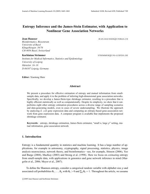
Figure 2: Left: Distribution of estimated mutual information values for all 5151 gene pairs of <strong>the</strong><br />
E. coli data set. Right: Mutual information values after applying <strong>the</strong> ARACNE gene<br />
pair selection procedure. Note that <strong>the</strong> most MIs have been set <strong>to</strong> zero by <strong>the</strong> ARACNE<br />
algorithm.<br />
For illustration, we now analyze data from Schmidt-Heck et al. (2004) who conducted an experiment<br />
<strong>to</strong> observe <strong>the</strong> stress response in E. Coli during expression of a recombinant protein. This<br />
1477
HAUSSER AND STRIMMER<br />
data set was also used in previous linear network analyzes, for example, in Schäfer <strong>and</strong> Strimmer<br />
(2005b). The raw data consist of 4289 protein coding genes, on which measurements were taken<br />
at 0, 8, 15, 22, 45, 68, 90, 150, <strong>and</strong> 180 minutes. We focus on a subset of G = 102 differentially<br />
expressed genes as given in Schmidt-Heck et al. (2004).<br />
Discretization of <strong>the</strong> data according <strong>to</strong> Freedman <strong>and</strong> Diaconis (1981) yielded K = 16 distinct<br />
gene expression levels. From <strong>the</strong> G = 102 genes, we estimated MIs for 5151 pairs of genes. For each<br />
pair, <strong>the</strong> mutual information was based on an estimated 16 × 16 contingency table, hence p = 256.<br />
As <strong>the</strong> number of time points is n = 9, this is a strongly undersampled situation which requires <strong>the</strong><br />
use of a regularized estimate of entropy <strong>and</strong> mutual information.<br />
The distribution of <strong>the</strong> shrinkage estimates of mutual information for all 5151 gene pairs is<br />
shown in <strong>the</strong> left side of Figure 2. The right h<strong>and</strong> side depicts <strong>the</strong> distribution of mutual information<br />
values after applying <strong>the</strong> ARACNE procedure, which yields 112 gene pairs <strong>with</strong> nonzero MIs.<br />
The model selection provided by ARACNE is based on applying <strong>the</strong> information processing<br />
inequality <strong>to</strong> all gene triplets. For each triplet, <strong>the</strong> gene pair corresponding <strong>to</strong> <strong>the</strong> smallest MI is discarded,<br />
which has <strong>the</strong> effect <strong>to</strong> remove gene-gene links that correspond <strong>to</strong> indirect ra<strong>the</strong>r than direct<br />
interactions. This is similar <strong>to</strong> a procedure used in graphical Gaussian models where correlations<br />
are transformed in<strong>to</strong> partial correlations. Thus, both <strong>the</strong> ARACNE <strong>and</strong> <strong>the</strong> MRNET algorithms can<br />
be considered as devices <strong>to</strong> approximate <strong>the</strong> conditional mutual information (Meyer et al., 2007).<br />
As a result, <strong>the</strong> 112 nonzero MIs recovered by <strong>the</strong> ARACNE algorithm correspond <strong>to</strong> statistically<br />
detectable direct associations.<br />
The corresponding gene association network is depicted in Figure 3. The most striking feature<br />
of <strong>the</strong> graph are <strong>the</strong> “hubs” belonging <strong>to</strong> genes hupB, sucA <strong>and</strong> nuoL. hupB is a well known DNAbinding<br />
transcriptional regula<strong>to</strong>r, whereas both nuoL <strong>and</strong> sucA are key components of <strong>the</strong> E. coli<br />
metabolism. Note that a Lasso-type procedure (that implicitly limits <strong>the</strong> number of edges that can<br />
connect <strong>to</strong> each node) such as that of Meinshausen <strong>and</strong> Bühlmann (2006) cannot recover <strong>the</strong>se hubs.<br />
6. Discussion<br />
We proposed a <strong>James</strong>-<strong>Stein</strong>-type shrinkage estima<strong>to</strong>r for inferring entropy <strong>and</strong> mutual information<br />
from small samples. While this is a challenging problem, we showed that our approach is highly<br />
efficient both statistically <strong>and</strong> computationally despite its simplicity.<br />
In terms of versatility, our estima<strong>to</strong>r has two distinct advantages over <strong>the</strong> NSB <strong>and</strong> Chao-Shen<br />
estima<strong>to</strong>rs. First, in addition <strong>to</strong> estimating <strong>the</strong> entropy, it also provides <strong>the</strong> underlying multinomial<br />
frequencies for use <strong>with</strong> <strong>the</strong> Shannon formula (Equation 1). This is useful in <strong>the</strong> context of using<br />
mutual information <strong>to</strong> quantify non-linear pairwise dependencies for instance. Second, unlike NSB,<br />
it is a fully analytic estima<strong>to</strong>r.<br />
Hence, our estima<strong>to</strong>r suggests itself for applications in large scale estimation problems. To<br />
demonstrate its application in <strong>the</strong> context of genomics <strong>and</strong> systems biology, we have estimated an<br />
entropy-based gene dependency network from expression data in E. coli. This type of approach may<br />
prove helpful <strong>to</strong> overcome <strong>the</strong> limitations of linear models currently used in network analysis.<br />
In short, we believe <strong>the</strong> proposed small-sample entropy estima<strong>to</strong>r will be a valuable contribution<br />
<strong>to</strong> <strong>the</strong> growing <strong>to</strong>olbox of machine learning <strong>and</strong> statistics procedures for high-dimensional data<br />
analysis.<br />
1478
ENTROPY INFERENCE AND THE JAMES-STEIN ESTIMATOR<br />
<br />
<br />
<br />
<br />
<br />
<br />
<br />
<br />
<br />
<br />
<br />
<br />
<br />
<br />
<br />
<br />
<br />
<br />
<br />
<br />
<br />
<br />
<br />
<br />
<br />
<br />
<br />
<br />
<br />
<br />
<br />
<br />
<br />
<br />
<br />
<br />
<br />
<br />
<br />
<br />
<br />
<br />
<br />
<br />
<br />
<br />
<br />
<br />
<br />
<br />
<br />
<br />
<br />
<br />
<br />
<br />
<br />
<br />
<br />
<br />
<br />
<br />
<br />
<br />
<br />
<br />
<br />
<br />
<br />
<br />
<br />
<br />
<br />
<br />
<br />
<br />
<br />
<br />
<br />
<br />
<br />
<br />
<br />
<br />
<br />
<br />
<br />
<br />
<br />
<br />
<br />
<br />
<br />
<br />
<br />
<br />
<br />
<br />
<br />
<br />
<br />
<br />
Figure 3: Mutual information network for <strong>the</strong> E. coli data inferred by <strong>the</strong> ARACNE algorithm based<br />
on shrinkage estimates of entropy <strong>and</strong> mutual information.<br />
1479
HAUSSER AND STRIMMER<br />
Acknowledgments<br />
This work was partially supported by a Emmy Noe<strong>the</strong>r grant of <strong>the</strong> Deutsche Forschungsgemeinschaft<br />
(<strong>to</strong> K.S.). We thank <strong>the</strong> anonymous referees <strong>and</strong> <strong>the</strong> edi<strong>to</strong>r for very helpful comments.<br />
Appendix A. Recipe For Constructing <strong>James</strong>-<strong>Stein</strong>-type Shrinkage <strong>Estima<strong>to</strong>r</strong>s<br />
The original <strong>James</strong>-<strong>Stein</strong> estima<strong>to</strong>r (<strong>James</strong> <strong>and</strong> <strong>Stein</strong>, 1961) was proposed <strong>to</strong> estimate <strong>the</strong> mean of<br />
a multivariate normal distribution from a single (n = 1!) vec<strong>to</strong>r observation. Specifically, if x is a<br />
sample from N p (µ,I) <strong>the</strong>n <strong>James</strong>-<strong>Stein</strong> estima<strong>to</strong>r is given by<br />
ˆµ JS<br />
k = (1 − p − 2<br />
∑ p )x k .<br />
k=1 x2 k<br />
Intriguingly, this estima<strong>to</strong>r outperforms <strong>the</strong> maximum likelihood estima<strong>to</strong>r ˆµ ML<br />
k<br />
= x k in terms of<br />
mean squared error if <strong>the</strong> dimension is p ≥ 3. Hence, <strong>the</strong> <strong>James</strong>-<strong>Stein</strong> estima<strong>to</strong>r dominates <strong>the</strong><br />
maximum likelihood estima<strong>to</strong>r.<br />
The above estima<strong>to</strong>r can be slightly generalized by shrinking <strong>to</strong>wards <strong>the</strong> component average<br />
¯x = ∑ p k=1 x k ra<strong>the</strong>r than <strong>to</strong> zero, resulting in<br />
<strong>with</strong> estimated shrinkage intensity<br />
ˆµ Shrink<br />
k<br />
ˆλ ⋆ =<br />
= ˆλ ⋆ ¯x+(1 − ˆλ ⋆ )x k<br />
p − 3<br />
∑ p k=1 (x k − ¯x) 2.<br />
The <strong>James</strong>-<strong>Stein</strong> shrinkage principle is very general <strong>and</strong> can be put <strong>to</strong> <strong>to</strong> use in many o<strong>the</strong>r<br />
high-dimensional settings. In <strong>the</strong> following we summarize a simple recipe for constructing <strong>James</strong>-<br />
<strong>Stein</strong>-type shrinkage estima<strong>to</strong>rs along <strong>the</strong> lines of Schäfer <strong>and</strong> Strimmer (2005b) <strong>and</strong> Opgen-Rhein<br />
<strong>and</strong> Strimmer (2007a).<br />
In short, <strong>the</strong>re are two key ideas at work in <strong>James</strong>-<strong>Stein</strong> shrinkage:<br />
i) regularization of a high-dimensional estima<strong>to</strong>r ˆθ by linear combination <strong>with</strong> a lowerdimensional<br />
target estimate ˆθ Target , <strong>and</strong><br />
ii) adaptive estimation of <strong>the</strong> shrinkage parameter λ from <strong>the</strong> data by quadratic risk minimization.<br />
A general form of a <strong>James</strong>-<strong>Stein</strong>-type shrinkage estima<strong>to</strong>r is given by<br />
ˆθ Shrink = λˆθ Target +(1 − λ)ˆθ. (9)<br />
Note that ˆθ <strong>and</strong> ˆθ Target are two very different estima<strong>to</strong>rs (for <strong>the</strong> same underlying model!). ˆθ as a<br />
high-dimensional estimate <strong>with</strong> many independent components has low bias but for small samples<br />
a potentially large variance. In contrast, <strong>the</strong> target estimate ˆθ Target is low-dimensional <strong>and</strong> <strong>the</strong>refore<br />
is generally less variable than ˆθ but at <strong>the</strong> same time is also more biased. The <strong>James</strong>-<strong>Stein</strong> estimate<br />
1480
ENTROPY INFERENCE AND THE JAMES-STEIN ESTIMATOR<br />
is a weighted average of <strong>the</strong>se two estima<strong>to</strong>rs, where <strong>the</strong> weight is chosen in a data-driven fashion<br />
such that ˆθ Shrink is improved in terms of mean squared error relative <strong>to</strong> both ˆθ <strong>and</strong> ˆθ Target .<br />
A key advantage of <strong>James</strong>-<strong>Stein</strong>-type shrinkage is that <strong>the</strong> optimal shrinkage intensity λ ⋆ can be<br />
calculated analytically <strong>and</strong> <strong>with</strong>out knowing <strong>the</strong> true value θ, via<br />
λ ⋆ = ∑p k=1 Var(ˆθ k ) − Cov(ˆθ k , ˆθ Target<br />
k<br />
)+Bias(ˆθ k )E(ˆθ k − ˆθ Target<br />
∑ p k=1 E[(ˆθ k − ˆθ Target<br />
k<br />
) 2 ]<br />
k<br />
)<br />
. (10)<br />
A simple estimate of λ ⋆ is obtained by replacing all variances <strong>and</strong> covariances in Equation 10 <strong>with</strong><br />
<strong>the</strong>ir empirical counterparts, followed by truncation of ˆλ ⋆ at 1 (so that ˆλ ⋆ ≤ 1 always holds).<br />
Equation 10 is discussed in detail in Schäfer <strong>and</strong> Strimmer (2005b) <strong>and</strong> Opgen-Rhein <strong>and</strong> Strimmer<br />
(2007a). More specialized versions of it are treated, for example, in Ledoit <strong>and</strong> Wolf (2003) for<br />
unbiased ˆθ <strong>and</strong> in Thompson (1968) (unbiased, univariate case <strong>with</strong> deterministic target). A very<br />
early version (univariate <strong>with</strong> zero target) even predates <strong>the</strong> estima<strong>to</strong>r of <strong>James</strong> <strong>and</strong> <strong>Stein</strong>, see Goodman<br />
(1953). For <strong>the</strong> multinormal setting of <strong>James</strong> <strong>and</strong> <strong>Stein</strong> (1961), Equation 9 <strong>and</strong> Equation 10<br />
reduce <strong>to</strong> <strong>the</strong> shrinkage estima<strong>to</strong>r described in Stigler (1990).<br />
<strong>James</strong>-<strong>Stein</strong> shrinkage has an empirical Bayes interpretation (Efron <strong>and</strong> Morris, 1973). Note,<br />
however, that only <strong>the</strong> first two moments of <strong>the</strong> distributions of ˆθ Target <strong>and</strong> ˆθ need <strong>to</strong> be specified in<br />
Equation 10. Hence, <strong>James</strong>-<strong>Stein</strong> estimation may be viewed as a quasi-empirical Bayes approach<br />
(in <strong>the</strong> same sense as in quasi-likelihood, which also requires only <strong>the</strong> first two moments).<br />
Appendix B. Computer Implementation<br />
The proposed shrinkage estima<strong>to</strong>rs of entropy <strong>and</strong> mutual information, as well as all o<strong>the</strong>r investigated<br />
entropy estima<strong>to</strong>rs, have been implemented in R (R Development Core Team, 2008). A<br />
corresponding R package “entropy” was deposited in <strong>the</strong> R archive CRAN <strong>and</strong> is accessible at <strong>the</strong><br />
URL http://cran.r-project.org/web/packages/entropy/ under <strong>the</strong> GNU General Public<br />
License.<br />
References<br />
A. Agresti <strong>and</strong> D. B. Hitchcock. Bayesian inference for categorical data analysis. Statist. Meth.<br />
Appl., 14:297–330, 2005.<br />
A. J. Butte, P. Tamayo, D. Slonim, T. R. Golub, <strong>and</strong> I. S. Kohane. Discovering functional relationships<br />
between RNA expression <strong>and</strong> chemo<strong>the</strong>rapeutic susceptibility using relevance networks.<br />
Proc. Natl. Acad. Sci. USA, 97:12182–12186, 2000.<br />
A. Chao <strong>and</strong> T.-J. Shen. Nonparametric estimation of Shannon’s index of diversity when <strong>the</strong>re are<br />
unseen species. Environ. Ecol. Stat., 10:429–443, 2003.<br />
A. Dobra, C. Hans, B. Jones, J. R. Nevins, G. Yao, <strong>and</strong> M. West. Sparse graphical models for<br />
exploring gene expression data. J. Multiv. Anal., 90:196–212, 2004.<br />
B. Efron <strong>and</strong> C. N. Morris. <strong>Stein</strong>’s estimation rule <strong>and</strong> its competi<strong>to</strong>rs–an empirical Bayes approach.<br />
J. Amer. Statist. Assoc., 68:117–130, 1973.<br />
1481
HAUSSER AND STRIMMER<br />
S. E. Fienberg <strong>and</strong> P. W. Holl<strong>and</strong>. Simultaneous estimation of multinomial cell probabilities. J.<br />
Amer. Statist. Assoc., 68:683–691, 1973.<br />
D. Freedman <strong>and</strong> P. Diaconis. On <strong>the</strong> his<strong>to</strong>gram as a density estima<strong>to</strong>r: L2 <strong>the</strong>ory. Z. Wahrscheinlichkeits<strong>the</strong>orie<br />
verw. Gebiete, 57:453–476, 1981.<br />
N. Friedman. Inferring cellular networks using probabilistic graphical models. Science, 303:799–<br />
805, 2004.<br />
S. Geisser. On prior distributions for binary trials. The American Statistician, 38:244–251, 1984.<br />
A. Gelman, J. B. Carlin, H. S. Stern, <strong>and</strong> D. B. Rubin. Bayesian Data Analysis. Chapman &<br />
Hall/CRC, Boca Ra<strong>to</strong>n, 2nd edition, 2004.<br />
I. J. Good. The population frequencies of species <strong>and</strong> <strong>the</strong> estimation of population parameters.<br />
Biometrika, 40:237–264, 1953.<br />
L. A. Goodman. A simple method for improving some estima<strong>to</strong>rs. Ann. Math. Statist., 24:114–117,<br />
1953.<br />
M. H. J. Gruber. Improving Efficiency By Shrinkage. Marcel Dekker, Inc., New York, 1998.<br />
D. Holste, I. Große, <strong>and</strong> H. Herzel. Bayes’ estima<strong>to</strong>rs of generalized entropies. J. Phys. A: Math.<br />
Gen., 31:2551–2566, 1998.<br />
D. G. Horvitz <strong>and</strong> D. J. Thompson. A generalization of sampling <strong>with</strong>out replacement from a finite<br />
universe. J. Amer. Statist. Assoc., 47:663–685, 1952.<br />
W. <strong>James</strong> <strong>and</strong> C. <strong>Stein</strong>. Estimation <strong>with</strong> quadratic loss. In Proc. Fourth Berkeley Symp. Math.<br />
Statist. Probab., volume 1, pages 361–379, Berkeley, 1961. Univ. California Press.<br />
H. Jeffreys. An invariant form for <strong>the</strong> prior probability in estimation problems. Proc. Roc. Soc.<br />
(Lond.) A, 186:453–461, 1946.<br />
M. Kalisch <strong>and</strong> P. Bühlmann. Estimating high-dimensional directed acyclic graphs <strong>with</strong> <strong>the</strong> PCalgorithm.<br />
J. Machine Learn. Res., 8:613–636, 2007.<br />
R. E. Krichevsky <strong>and</strong> V. K. Trofimov. The performance of universal encoding. IEEE Trans. Inf.<br />
Theory, 27:199–207, 1981.<br />
H. Lähdesmäki <strong>and</strong> I. Shmulevich. Learning <strong>the</strong> structure of dynamic Bayesian networks from time<br />
series <strong>and</strong> steady state measurements. Mach. Learn., 71:185–217, 2008.<br />
O. Ledoit <strong>and</strong> M. Wolf. Improved estimation of <strong>the</strong> covariance matrix of s<strong>to</strong>ck returns <strong>with</strong> an<br />
application <strong>to</strong> portfolio selection. J. Empir. Finance, 10:603–621, 2003.<br />
D. J. C. MacKay. Information Theory, <strong>Inference</strong>, <strong>and</strong> Learning Algorithms. Cambridge University<br />
Press, Cambridge, 2003.<br />
A.A. Margolin, I. Nemenman, K. Basso, C. Wiggins, G. S<strong>to</strong>lovitzky, R. Dalla Favera, <strong>and</strong> A. Califano.<br />
ARACNE: an algorithm for <strong>the</strong> reconstruction of gene regula<strong>to</strong>ry networks in a mammalian<br />
cellular context. BMC Bioinformatics, 7 (Suppl. 1):S7, 2006.<br />
1482
ENTROPY INFERENCE AND THE JAMES-STEIN ESTIMATOR<br />
N. Meinshausen <strong>and</strong> P. Bühlmann. High-dimensional graphs <strong>and</strong> variable selection <strong>with</strong> <strong>the</strong> Lasso.<br />
Ann. Statist., 34:1436–1462, 2006.<br />
P. E. Meyer, K. Kon<strong>to</strong>s, F. Lafitte, <strong>and</strong> G. Bontempi. Information-<strong>the</strong>oretic inference of large transcriptional<br />
regula<strong>to</strong>ry networks. EURASIP J. Bioinf. Sys. Biol., page doi:10.1155/2007/79879,<br />
2007.<br />
G. A. Miller. Note on <strong>the</strong> bias of information estimates. In H. Quastler, edi<strong>to</strong>r, Information Theory<br />
in Psychology II-B, pages 95–100. Free Press, Glencoe, IL, 1955.<br />
I. Nemenman, F. Shafee, <strong>and</strong> W. Bialek. <strong>Entropy</strong> <strong>and</strong> inference, revisited. In T. G. Dietterich,<br />
S. Becker, <strong>and</strong> Z. Ghahramani, edi<strong>to</strong>rs, Advances in Neural Information Processing Systems 14,<br />
pages 471–478, Cambridge, MA, 2002. MIT Press.<br />
R. Opgen-Rhein <strong>and</strong> K. Strimmer. Accurate ranking of differentially expressed genes by a<br />
distribution-free shrinkage approach. Statist. Appl. Genet. Mol. Biol., 6:9, 2007a.<br />
R. Opgen-Rhein <strong>and</strong> K. Strimmer. From correlation <strong>to</strong> causation networks: a simple approximate<br />
learning algorithm <strong>and</strong> its application <strong>to</strong> high-dimensional plant gene expression data. BMC<br />
Systems Biology, 1:37, 2007b.<br />
A. Orlitsky, N. P. Santhanam, <strong>and</strong> J. Zhang. Always Good Turing: asymp<strong>to</strong>tically optimal probability<br />
estimation. Science, 302:427–431, 2003.<br />
W. Perks. Some observations on inverse probability including a new indifference rule. J. Inst.<br />
Actuaries, 73:285–334, 1947.<br />
R Development Core Team. R: A Language <strong>and</strong> Environment for Statistical Computing. R Foundation<br />
for Statistical Computing, Vienna, Austria, 2008. URL http://www.R-project.org.<br />
ISBN 3-900051-07-0.<br />
C. Rangel, J. Angus, Z. Ghahramani, M. Lioumi, E. So<strong>the</strong>ran, A. Gaiba, D. L. Wild, <strong>and</strong> F. Falciani.<br />
Modeling T-cell activation using gene expression profiling <strong>and</strong> state space modeling. Bioinformatics,<br />
20:1361–1372, 2004.<br />
J. Schäfer <strong>and</strong> K. Strimmer. An empirical Bayes approach <strong>to</strong> inferring large-scale gene association<br />
networks. Bioinformatics, 21:754–764, 2005a.<br />
J. Schäfer <strong>and</strong> K. Strimmer. A shrinkage approach <strong>to</strong> large-scale covariance matrix estimation <strong>and</strong><br />
implications for functional genomics. Statist. Appl. Genet. Mol. Biol., 4:32, 2005b.<br />
W. Schmidt-Heck, R. Guthke, S. Toepfer, H. Reischer, K. Duerrschmid, <strong>and</strong> K. Bayer. Reverse<br />
engineering of <strong>the</strong> stress response during expression of a recombinant protein. In Proceedings<br />
of <strong>the</strong> EUNITE symposium, 10-12 June 2004, Aachen, Germany, pages 407–412, 2004. Verlag<br />
Mainz.<br />
T. Schürmann <strong>and</strong> P. Grassberger. <strong>Entropy</strong> estimation of symbol sequences. Chaos, 6:414–427,<br />
1996.<br />
S. M. Stigler. A Gal<strong>to</strong>nian perspective on shrinkage estima<strong>to</strong>rs. Statistical Science, 5:147–155,<br />
1990.<br />
1483
HAUSSER AND STRIMMER<br />
D.R. Stinson. Cryp<strong>to</strong>graphy: Theory <strong>and</strong> Practice. CRC Press, 2006.<br />
S. P. Strong, R. Koberle, R. de Ruyter van Steveninck, <strong>and</strong> W. Bialek. <strong>Entropy</strong> <strong>and</strong> information in<br />
neural spike trains. Phys. Rev. Letters, 80:197–200, 1998.<br />
J. R. Thompson. Some shrinkage techniques for estimating <strong>the</strong> mean. J. Amer. Statist. Assoc., 63:<br />
113–122, 1968.<br />
S. Trybula. Some problems of simultaneous minimax estimation. Ann. Math. Statist., 29:245–253,<br />
1958.<br />
F. Tuyl, R. Gerlach, <strong>and</strong> K. Mengersen. A comparison of Bayes-Laplace, Jeffreys, <strong>and</strong> o<strong>the</strong>r priors:<br />
<strong>the</strong> case of zero events. The American Statistician, 62:40–44, 2008.<br />
V. Q. Vu, B. Yu, <strong>and</strong> R. E. Kass. Coverage-adjusted entropy estimation. Stat. Med., 26:4039–4060,<br />
2007.<br />
G. Yeo <strong>and</strong> C. B. Burge. Maximum entropy modeling of short sequence motifs <strong>with</strong> applications <strong>to</strong><br />
RNA splicing signals. J. Comp. Biol., 11:377–394, 2004.<br />
1484