Entropy Inference and the James-Stein Estimator, with Application to ...
Entropy Inference and the James-Stein Estimator, with Application to ...
Entropy Inference and the James-Stein Estimator, with Application to ...

You also want an ePaper? Increase the reach of your titles
YUMPU automatically turns print PDFs into web optimized ePapers that Google loves.
Journal of Machine Learning Research 10 (2009) 1469-1484 Submitted 10/08; Revised 4/09; Published 7/09<br />
<strong>Entropy</strong> <strong>Inference</strong> <strong>and</strong> <strong>the</strong> <strong>James</strong>-<strong>Stein</strong> <strong>Estima<strong>to</strong>r</strong>, <strong>with</strong> <strong>Application</strong> <strong>to</strong><br />
Nonlinear Gene Association Networks<br />
Jean Hausser<br />
Bioinformatics, Biozentrum<br />
University of Basel<br />
Klingelbergstr. 50/70<br />
CH-4056 Basel, Switzerl<strong>and</strong><br />
Korbinian Strimmer<br />
Institute for Medical Informatics, Statistics <strong>and</strong> Epidemiology<br />
University of Leipzig<br />
Härtelstr. 16–18<br />
D-04107 Leipzig, Germany<br />
JEAN.HAUSSER@UNIBAS.CH<br />
STRIMMER@UNI-LEIPZIG.DE<br />
Edi<strong>to</strong>r: Xiao<strong>to</strong>ng Shen<br />
Abstract<br />
We present a procedure for effective estimation of entropy <strong>and</strong> mutual information from smallsample<br />
data, <strong>and</strong> apply it <strong>to</strong> <strong>the</strong> problem of inferring high-dimensional gene association networks.<br />
Specifically, we develop a <strong>James</strong>-<strong>Stein</strong>-type shrinkage estima<strong>to</strong>r, resulting in a procedure that is<br />
highly efficient statistically as well as computationally. Despite its simplicity, we show that it outperforms<br />
eight o<strong>the</strong>r entropy estimation procedures across a diverse range of sampling scenarios<br />
<strong>and</strong> data-generating models, even in cases of severe undersampling. We illustrate <strong>the</strong> approach<br />
by analyzing E. coli gene expression data <strong>and</strong> computing an entropy-based gene-association network<br />
from gene expression data. A computer program is available that implements <strong>the</strong> proposed<br />
shrinkage estima<strong>to</strong>r.<br />
Keywords: entropy, shrinkage estimation, <strong>James</strong>-<strong>Stein</strong> estima<strong>to</strong>r, “small n, large p” setting, mutual<br />
information, gene association network<br />
1. Introduction<br />
<strong>Entropy</strong> is a fundamental quantity in statistics <strong>and</strong> machine learning. It has a large number of applications,<br />
for example in astronomy, cryp<strong>to</strong>graphy, signal processing, statistics, physics, image<br />
analysis neuroscience, network <strong>the</strong>ory, <strong>and</strong> bioinformatics—see, for example, Stinson (2006), Yeo<br />
<strong>and</strong> Burge (2004), MacKay (2003) <strong>and</strong> Strong et al. (1998). Here we focus on estimating entropy<br />
from small-sample data, <strong>with</strong> applications in genomics <strong>and</strong> gene network inference in mind (Margolin<br />
et al., 2006; Meyer et al., 2007).<br />
To define <strong>the</strong> Shannon entropy, consider a categorical r<strong>and</strong>om variable <strong>with</strong> alphabet size p <strong>and</strong><br />
associated cell probabilities θ 1 ,...,θ p <strong>with</strong> θ k > 0 <strong>and</strong> ∑ k θ k = 1. Throughout <strong>the</strong> article, we assume<br />
c○2009 Jean Hausser <strong>and</strong> Korbinian Strimmer.
HAUSSER AND STRIMMER<br />
that p is fixed <strong>and</strong> known. In this setting, <strong>the</strong> Shannon entropy in natural units is given by 1<br />
H = −<br />
p<br />
∑<br />
k=1<br />
θ k log(θ k ). (1)<br />
In practice, <strong>the</strong> underlying probability mass function are unknown, hence H <strong>and</strong> θ k need <strong>to</strong> be<br />
estimated from observed cell counts y k ≥ 0.<br />
A particularly simple <strong>and</strong> widely used estima<strong>to</strong>r of entropy is <strong>the</strong> maximum likelihood (ML)<br />
estima<strong>to</strong>r<br />
Ĥ ML = −<br />
p<br />
∑<br />
k=1<br />
constructed by plugging <strong>the</strong> ML frequency estimates<br />
ˆθ ML<br />
k log(ˆθ ML<br />
k )<br />
ˆθ ML<br />
k<br />
= y k<br />
n<br />
(2)<br />
in<strong>to</strong> Equation 1, <strong>with</strong> n = ∑ p k=1 y k being <strong>the</strong> <strong>to</strong>tal number of counts.<br />
In situations <strong>with</strong> n ≫ p, that is, when <strong>the</strong> dimension is low <strong>and</strong> when <strong>the</strong>re are many observation,<br />
it is easy <strong>to</strong> infer entropy reliably, <strong>and</strong> it is well-known that in this case <strong>the</strong> ML estima<strong>to</strong>r is<br />
optimal. However, in high-dimensional problems <strong>with</strong> n ≪ p it becomes extremely challenging <strong>to</strong><br />
estimate <strong>the</strong> entropy. Specifically, in <strong>the</strong> “small n, large p” regime <strong>the</strong> ML estima<strong>to</strong>r performs very<br />
poorly <strong>and</strong> severely underestimates <strong>the</strong> true entropy.<br />
While entropy estimation has a long his<strong>to</strong>ry tracing back <strong>to</strong> more than 50 years ago, it is only<br />
recently that <strong>the</strong> specific issues arising in high-dimensional, undersampled data sets have attracted<br />
attention. This has lead <strong>to</strong> two recent innovations, namely <strong>the</strong> NSB algorithm (Nemenman et al.,<br />
2002) <strong>and</strong> <strong>the</strong> Chao-Shen estima<strong>to</strong>r (Chao <strong>and</strong> Shen, 2003), both of which are now widely considered<br />
as benchmarks for <strong>the</strong> small-sample entropy estimation problem (Vu et al., 2007).<br />
Here, we introduce a novel <strong>and</strong> highly efficient small-sample entropy estima<strong>to</strong>r based on <strong>James</strong>-<br />
<strong>Stein</strong> shrinkage (Gruber, 1998). Our method is fully analytic <strong>and</strong> hence computationally inexpensive.<br />
Moreover, our procedure simultaneously provides estimates of <strong>the</strong> entropy <strong>and</strong> of <strong>the</strong> cell<br />
frequencies suitable for plugging in<strong>to</strong> <strong>the</strong> Shannon entropy formula (Equation 1). Thus, in comparison<br />
<strong>the</strong> estima<strong>to</strong>r we propose is simpler, very efficient, <strong>and</strong> at <strong>the</strong> same time more versatile than<br />
currently available entropy estima<strong>to</strong>rs.<br />
2. Conventional Methods for Estimating <strong>Entropy</strong><br />
<strong>Entropy</strong> estima<strong>to</strong>rs can be divided in<strong>to</strong> two groups: i) methods, that rely on estimates of cell frequencies,<br />
<strong>and</strong> ii) estima<strong>to</strong>rs, that directly infer entropy <strong>with</strong>out estimating a compatible set of θ k .<br />
Most methods discussed below fall in<strong>to</strong> <strong>the</strong> first group, except for <strong>the</strong> Miller-Madow <strong>and</strong> NSB<br />
approaches.<br />
1. In this paper we use <strong>the</strong> following conventions: log denotes <strong>the</strong> natural logarithm (not base 2 or base 10), <strong>and</strong> we<br />
define 0log0 = 0.<br />
1470
ENTROPY INFERENCE AND THE JAMES-STEIN ESTIMATOR<br />
2.1 Maximum Likelihood Estimate<br />
The connection between observed counts y k <strong>and</strong> frequencies θ k is given by <strong>the</strong> multinomial distribution<br />
p<br />
n!<br />
Prob(y 1 ,...,y p ;θ 1 ,...,θ p ) =<br />
∏ p k=1 y ∏ θ y k<br />
k<br />
k!<br />
. (3)<br />
Note that θ k > 0 because o<strong>the</strong>rwise <strong>the</strong> distribution is singular. In contrast, <strong>the</strong>re may be (<strong>and</strong><br />
often are) zero counts y k . The ML estima<strong>to</strong>r of θ k maximizes <strong>the</strong> right h<strong>and</strong> side of Equation 3 for<br />
fixed y k , leading <strong>to</strong> <strong>the</strong> observed frequencies ˆθ ML<br />
k<br />
= y k<br />
n<br />
<strong>with</strong> variances Var(ˆθ ML<br />
k<br />
) = 1 n θ k(1 − θ k ) <strong>and</strong><br />
Bias(ˆθ ML<br />
k<br />
) = 0 as E(ˆθ ML<br />
k<br />
) = θ k .<br />
2.2 Miller-Madow <strong>Estima<strong>to</strong>r</strong><br />
While ˆθ ML<br />
k<br />
is unbiased, <strong>the</strong> corresponding plugin entropy estima<strong>to</strong>r Ĥ ML is not. First order bias<br />
correction leads <strong>to</strong><br />
Ĥ MM = Ĥ ML + m >0 − 1<br />
,<br />
2n<br />
where m >0 is <strong>the</strong> number of cells <strong>with</strong> y k > 0. This is known as <strong>the</strong> Miller-Madow estima<strong>to</strong>r (Miller,<br />
1955).<br />
2.3 Bayesian <strong>Estima<strong>to</strong>r</strong>s<br />
Bayesian regularization of cell counts may lead <strong>to</strong> vast improvements over <strong>the</strong> ML estima<strong>to</strong>r (Agresti<br />
<strong>and</strong> Hitchcock, 2005). Using <strong>the</strong> Dirichlet distribution <strong>with</strong> parameters a 1 ,a 2 ,...,a p as prior, <strong>the</strong><br />
resulting posterior distribution is also Dirichlet <strong>with</strong> mean<br />
ˆθ Bayes<br />
k<br />
= y k + a k<br />
n+A ,<br />
where A = ∑ p k=1 a k. The flattening constants a k play <strong>the</strong> role of pseudo-counts (compare <strong>with</strong> Equation<br />
2), so that A may be interpreted as <strong>the</strong> a priori sample size.<br />
Some common choices for a k are listed in Table 1, along <strong>with</strong> references <strong>to</strong> <strong>the</strong> corresponding<br />
plugin entropy estima<strong>to</strong>rs,<br />
Ĥ Bayes = −<br />
p<br />
∑<br />
k=1<br />
ˆθ Bayes<br />
k<br />
log(ˆθ Bayes<br />
k<br />
).<br />
k=1<br />
a k Cell frequency prior <strong>Entropy</strong> estima<strong>to</strong>r<br />
0 no prior maximum likelihood<br />
1/2 Jeffreys prior (Jeffreys, 1946) Krichevsky <strong>and</strong> Trofimov (1981)<br />
1 Bayes-Laplace uniform prior Holste et al. (1998)<br />
1/p Perks prior (Perks, 1947) Schürmann <strong>and</strong> Grassberger (1996)<br />
√ n/p minimax prior (Trybula, 1958)<br />
Table 1: Common choices for <strong>the</strong> parameters of <strong>the</strong> Dirichlet prior in <strong>the</strong> Bayesian estima<strong>to</strong>rs of<br />
cell frequencies, <strong>and</strong> corresponding entropy estima<strong>to</strong>rs.<br />
1471
HAUSSER AND STRIMMER<br />
While <strong>the</strong> multinomial model <strong>with</strong> Dirichlet prior is st<strong>and</strong>ard Bayesian folklore (Gelman et al.,<br />
2004), <strong>the</strong>re is no general agreement regarding which assignment of a k is best as noninformative<br />
prior—see for instance <strong>the</strong> discussion in Tuyl et al. (2008) <strong>and</strong> Geisser (1984). But, as shown later<br />
in this article, choosing inappropriate a k can easily cause <strong>the</strong> resulting estima<strong>to</strong>r <strong>to</strong> perform worse<br />
than <strong>the</strong> ML estima<strong>to</strong>r, <strong>the</strong>reby defeating <strong>the</strong> originally intended purpose.<br />
2.4 NSB <strong>Estima<strong>to</strong>r</strong><br />
The NSB approach (Nemenman et al., 2002) avoids overrelying on a particular choice of a k in <strong>the</strong><br />
Bayes estima<strong>to</strong>r by using a more refined prior. Specifically, a Dirichlet mixture prior <strong>with</strong> infinite<br />
number of components is employed, constructed such that <strong>the</strong> resulting prior over <strong>the</strong> entropy is<br />
uniform. While <strong>the</strong> NSB estima<strong>to</strong>r is one of <strong>the</strong> best entropy estima<strong>to</strong>rs available at present in<br />
terms of statistical properties, using <strong>the</strong> Dirichlet mixture prior is computationally expensive <strong>and</strong><br />
somewhat slow for practical applications.<br />
2.5 Chao-Shen <strong>Estima<strong>to</strong>r</strong><br />
Ano<strong>the</strong>r recently proposed estima<strong>to</strong>r is due <strong>to</strong> Chao <strong>and</strong> Shen (2003). This approach applies <strong>the</strong><br />
Horvitz-Thompson estima<strong>to</strong>r (Horvitz <strong>and</strong> Thompson, 1952) in combination <strong>with</strong> <strong>the</strong> Good-Turing<br />
correction (Good, 1953; Orlitsky et al., 2003) of <strong>the</strong> empirical cell probabilities <strong>to</strong> <strong>the</strong> problem of<br />
entropy estimation. The Good-Turing-corrected frequency estimates are<br />
ˆθ GT<br />
k = (1 − m 1 ML<br />
)ˆθ k ,<br />
n<br />
where m 1 is <strong>the</strong> number of single<strong>to</strong>ns, that is, cells <strong>with</strong> y k = 1. Used jointly <strong>with</strong> <strong>the</strong> Horvitz-<br />
Thompson estima<strong>to</strong>r this results in<br />
Ĥ CS = −<br />
p<br />
∑<br />
k=1<br />
ˆθ GT<br />
k<br />
log ˆθ GT<br />
k<br />
(1 −(1 − ˆθ GT<br />
k<br />
) n ) ,<br />
an estima<strong>to</strong>r <strong>with</strong> remarkably good statistical properties (Vu et al., 2007).<br />
3. A <strong>James</strong>-<strong>Stein</strong> Shrinkage <strong>Estima<strong>to</strong>r</strong><br />
The contribution of this paper is <strong>to</strong> introduce an entropy estima<strong>to</strong>r that employs <strong>James</strong>-<strong>Stein</strong>-type<br />
shrinkage at <strong>the</strong> level of cell frequencies. As we will show below, this leads <strong>to</strong> an entropy estima<strong>to</strong>r<br />
that is highly effective, both in terms of statistical accuracy <strong>and</strong> computational complexity.<br />
<strong>James</strong>-<strong>Stein</strong>-type shrinkage is a simple analytic device <strong>to</strong> perform regularized high-dimensional<br />
inference. It is ideally suited for small-sample settings - <strong>the</strong> original estima<strong>to</strong>r (<strong>James</strong> <strong>and</strong> <strong>Stein</strong>,<br />
1961) considered sample size n = 1. A general recipe for constructing shrinkage estima<strong>to</strong>rs is given<br />
in Appendix A. In this section, we describe how this approach can be applied <strong>to</strong> <strong>the</strong> specific problem<br />
of estimating cell frequencies.<br />
<strong>James</strong>-<strong>Stein</strong> shrinkage is based on averaging two very different models: a high-dimensional<br />
model <strong>with</strong> low bias <strong>and</strong> high variance, <strong>and</strong> a lower dimensional model <strong>with</strong> larger bias but smaller<br />
variance. The intensity of <strong>the</strong> regularization is determined by <strong>the</strong> relative weighting of <strong>the</strong> two<br />
models. Here we consider <strong>the</strong> convex combination<br />
ˆθ Shrink<br />
k<br />
= λt k +(1 − λ)ˆθ ML<br />
k , (4)<br />
1472
ENTROPY INFERENCE AND THE JAMES-STEIN ESTIMATOR<br />
where λ ∈ [0,1] is <strong>the</strong> shrinkage intensity that takes on a value between 0 (no shrinkage) <strong>and</strong> 1<br />
(full shrinkage), <strong>and</strong> t k is <strong>the</strong> shrinkage target. A convenient choice of t k is <strong>the</strong> uniform distribution<br />
t k = 1 p<br />
. This is also <strong>the</strong> maximum entropy target. Considering that Bias(ˆθ<br />
ML<br />
k<br />
) = 0 <strong>and</strong> using <strong>the</strong><br />
unbiased estima<strong>to</strong>r ̂Var(ˆθ ML<br />
k<br />
) =<br />
ˆθ ML<br />
k<br />
(1−ˆθ ML<br />
k )<br />
n−1<br />
we obtain (cf. Appendix A) for <strong>the</strong> shrinkage intensity<br />
ˆλ ⋆ = ∑p k=1 ̂Var(ˆθ<br />
ML<br />
k<br />
)<br />
∑ p k=1 (t k − ˆθ ML<br />
k<br />
) = 1 − ∑ p k=1<br />
(ˆθ<br />
ML<br />
k<br />
) 2<br />
2 (n − 1)∑ p k=1 (t k − ˆθ ML<br />
(5)<br />
k<br />
) 2.<br />
Note that this also assumes a non-s<strong>to</strong>chastic target t k . The resulting plugin shrinkage entropy estimate<br />
is<br />
Ĥ Shrink = −<br />
p<br />
∑<br />
k=1<br />
ˆθ Shrink<br />
k log(ˆθ Shrink<br />
k ). (6)<br />
Remark 1 There is a one <strong>to</strong> one correspondence between <strong>the</strong> shrinkage <strong>and</strong> <strong>the</strong> Bayes estima<strong>to</strong>r. If<br />
we write t k = a k<br />
A <strong>and</strong> λ = A<br />
n+A , <strong>the</strong>n ˆθ Shrink<br />
k<br />
= ˆθ Bayes<br />
k<br />
. This implies that <strong>the</strong> shrinkage estima<strong>to</strong>r is an<br />
empirical Bayes estima<strong>to</strong>r <strong>with</strong> a data-driven choice of <strong>the</strong> flattening constants—see also Efron <strong>and</strong><br />
Morris (1973). For every choice of A <strong>the</strong>re exists an equivalent shrinkage intensity λ. Conversely,<br />
for every λ <strong>the</strong>re exist an equivalent A = n λ<br />
1−λ .<br />
Remark 2 Developing A = n λ<br />
1−λ = n(λ + λ2 + ...) we obtain <strong>the</strong> approximate estimate  = nˆλ,<br />
which in turn recovers <strong>the</strong> “pseudo-Bayes” estima<strong>to</strong>r described in Fienberg <strong>and</strong> Holl<strong>and</strong> (1973).<br />
Remark 3 The shrinkage estima<strong>to</strong>r assumes a fixed <strong>and</strong> known p. In many practical applications<br />
this will indeed be <strong>the</strong> case, for example, if <strong>the</strong> observed counts are due <strong>to</strong> discretization (see also<br />
<strong>the</strong> data example). In addition, <strong>the</strong> shrinkage estima<strong>to</strong>r appears <strong>to</strong> be robust against assuming a<br />
larger p than necessary (see scenario 3 in <strong>the</strong> simulations).<br />
Remark 4 The shrinkage approach can easily be modified <strong>to</strong> allow multiple targets <strong>with</strong> different<br />
shrinkage intensities. For instance, using <strong>the</strong> Good-Turing estima<strong>to</strong>r (Good, 1953; Orlitsky et al.,<br />
2003), one could setup a different uniform target for <strong>the</strong> non-zero <strong>and</strong> <strong>the</strong> zero counts, respectively.<br />
4. Comparative Evaluation of Statistical Properties<br />
In order <strong>to</strong> elucidate <strong>the</strong> relative strengths <strong>and</strong> weaknesses of <strong>the</strong> entropy estima<strong>to</strong>rs reviewed in <strong>the</strong><br />
previous section, we set <strong>to</strong> benchmark <strong>the</strong>m in a simulation study covering different data generation<br />
processes <strong>and</strong> sampling regimes.<br />
4.1 Simulation Setup<br />
We compared <strong>the</strong> statistical performance of all nine described estima<strong>to</strong>rs (maximum likelihood,<br />
Miller-Madow, four Bayesian estima<strong>to</strong>rs, <strong>the</strong> proposed shrinkage estima<strong>to</strong>r (Equations 4–6), NSB<br />
und Chao-Shen) under various sampling <strong>and</strong> data generating scenarios:<br />
• The dimension was fixed at p = 1000.<br />
• Samples size n varied from 10, 30, 100, 300, 1000, 3000, <strong>to</strong> 10000. That is, we investigate<br />
cases of dramatic undersampling (“small n, large p”) as well as situations <strong>with</strong> a larger number<br />
of observed counts.<br />
1473
HAUSSER AND STRIMMER<br />
The true cell probabilities θ 1 ,...,θ 1000 were assigned in four different fashions, corresponding <strong>to</strong><br />
rows 1-4 in Figure 1:<br />
1. Sparse <strong>and</strong> heterogeneous, following a Dirichlet distribution <strong>with</strong> parameter a = 0.0007,<br />
2. R<strong>and</strong>om <strong>and</strong> homogeneous, following a Dirichlet distribution <strong>with</strong> parameter a = 1,<br />
3. As in scenario 2, but <strong>with</strong> half of <strong>the</strong> cells containing structural zeros, <strong>and</strong><br />
4. Following a Zipf-type power law.<br />
For each sampling scenario <strong>and</strong> sample size, we conducted 1000 simulation runs. In each run, we<br />
generated a new set of true cell frequencies <strong>and</strong> subsequently sampled observed counts y k from <strong>the</strong><br />
corresponding multinomial distribution. The resulting counts y k were <strong>the</strong>n supplied <strong>to</strong> <strong>the</strong> various<br />
entropy <strong>and</strong> cell frequencies estima<strong>to</strong>rs <strong>and</strong> <strong>the</strong> squared error ∑ 1000<br />
i=k (θ k − ˆθ k ) 2 was computed. From<br />
<strong>the</strong> 1000 repetitions we estimated <strong>the</strong> mean squared error (MSE) of <strong>the</strong> cell frequencies by averaging<br />
over <strong>the</strong> individual squared errors (except for <strong>the</strong> NSB, Miller-Madow, <strong>and</strong> Chao-Shen estima<strong>to</strong>rs).<br />
Similarly, we computed estimates of MSE <strong>and</strong> bias of <strong>the</strong> inferred entropies.<br />
4.2 Summary of Results from Simulations<br />
Figure 1 displays <strong>the</strong> results of <strong>the</strong> simulation study, which can be summarized as follows:<br />
• Unsurprisingly, all estima<strong>to</strong>rs perform well when <strong>the</strong> sample size is large.<br />
• The maximum likelihood <strong>and</strong> Miller-Madow estima<strong>to</strong>rs perform worst, except for scenario 1.<br />
Note that <strong>the</strong>se estima<strong>to</strong>rs are inappropriate even for moderately large sample sizes. Fur<strong>the</strong>rmore,<br />
<strong>the</strong> bias correction of <strong>the</strong> Miller-Madow estima<strong>to</strong>r is not particularly effective.<br />
• The minimax <strong>and</strong> 1/p Bayesian estima<strong>to</strong>rs tend <strong>to</strong> perform slightly better than maximum<br />
likelihood, but not by much.<br />
• The Bayesian estima<strong>to</strong>rs <strong>with</strong> pseudocounts 1/2 <strong>and</strong> 1 perform very well even for small sample<br />
sizes in <strong>the</strong> scenarios 2 <strong>and</strong> 3. However, <strong>the</strong>y are less efficient in scenario 4, <strong>and</strong> completely<br />
fail in scenario 1.<br />
• Hence, <strong>the</strong> Bayesian estima<strong>to</strong>rs can perform better or worse than <strong>the</strong> ML estima<strong>to</strong>r, depending<br />
on <strong>the</strong> choice of <strong>the</strong> prior <strong>and</strong> on <strong>the</strong> sampling scenario.<br />
• The NSB, <strong>the</strong> Chao-Shen <strong>and</strong> <strong>the</strong> shrinkage estima<strong>to</strong>r all are statistically very efficient <strong>with</strong><br />
small MSEs in all four scenarios, regardless of sample size.<br />
• The NSB <strong>and</strong> Chao-Shen estima<strong>to</strong>rs are nearly unbiased in scenario 3.<br />
The three <strong>to</strong>p-performing estima<strong>to</strong>rs are <strong>the</strong> NSB, <strong>the</strong> Chao-Shen <strong>and</strong> <strong>the</strong> prosed shrinkage estima<strong>to</strong>r.<br />
When it comes <strong>to</strong> estimating <strong>the</strong> entropy, <strong>the</strong>se estima<strong>to</strong>rs can be considered identical for<br />
practical purposes. However, <strong>the</strong> shrinkage estima<strong>to</strong>r is <strong>the</strong> only one that simultaneously estimates<br />
cell frequencies suitable for use <strong>with</strong> <strong>the</strong> Shannon entropy formula (Equation 1), <strong>and</strong> it does so<br />
<strong>with</strong> high accuracy even for small samples. In comparison, <strong>the</strong> NSB estima<strong>to</strong>r is by far <strong>the</strong> slowest<br />
method: in our simulations, <strong>the</strong> shrinkage estima<strong>to</strong>r was faster by a fac<strong>to</strong>r of 1000.<br />
1474
ENTROPY INFERENCE AND THE JAMES-STEIN ESTIMATOR<br />
Probability density<br />
MSE cell frequencies<br />
MSE entropy<br />
Bias entropy<br />
probability<br />
0.0 0.2 0.4 0.6<br />
H = 1.11<br />
Dirichlet<br />
a=0.0007, p=1000<br />
estimated MSE<br />
0.0 0.2 0.4<br />
ML<br />
1/2<br />
1<br />
1/p<br />
minimax<br />
Shrink<br />
estimated MSE<br />
0 20 40 60 80<br />
Miller−Madow<br />
Chao−Shen<br />
NSB<br />
estimated Bias<br />
0 2 4 6 8<br />
0 200 400 600 800<br />
10 50 500 5000<br />
10 50 500 5000<br />
10 50 500 5000<br />
probability<br />
0.000 0.004 0.008<br />
H = 6.47<br />
Dirichlet<br />
a=1, p=1000<br />
estimated MSE<br />
0.00 0.04 0.08<br />
estimated MSE<br />
0 10 20 30<br />
estimated Bias<br />
−6 −4 −2 0<br />
0 200 400 600 800<br />
10 50 500 5000<br />
10 50 500 5000<br />
10 50 500 5000<br />
probability<br />
0.000 0.010 0.020<br />
Dirichlet<br />
a=1, p=500 + 500 zeros<br />
H = 5.77<br />
estimated MSE<br />
0.00 0.04 0.08<br />
estimated MSE<br />
0 5 10 15 20 25<br />
estimated Bias<br />
−5 −3 −1 0 1<br />
probability<br />
0.00 0.05 0.10 0.15<br />
0 200 400 600 800<br />
Zipf<br />
p=1000<br />
H = 5.19<br />
estimated MSE<br />
0.00 0.04 0.08<br />
10 50 500 5000<br />
estimated MSE<br />
0 5 10 15 20<br />
10 50 500 5000<br />
estimated Bias<br />
−4 −2 0 1 2<br />
10 50 500 5000<br />
0 200 400 600 800<br />
10 50 500 5000<br />
10 50 500 5000<br />
10 50 500 5000<br />
bin number<br />
sample size n<br />
sample size n<br />
sample size n<br />
Figure 1: Comparing <strong>the</strong> performance of nine different entropy estima<strong>to</strong>rs (maximum likelihood,<br />
Miller-Madow, four Bayesian estima<strong>to</strong>rs, <strong>the</strong> proposed shrinkage estima<strong>to</strong>r, NSB und<br />
Chao-Shen) in four different sampling scenarios (rows 1 <strong>to</strong> 4). The estima<strong>to</strong>rs are compared<br />
in terms of MSE of <strong>the</strong> underlying cell frequencies (except for Miller-Madow, NSB,<br />
Chao-Shen) <strong>and</strong> according <strong>to</strong> MSE <strong>and</strong> Bias of <strong>the</strong> estimated entropies. The dimension<br />
is fixed at p = 1000 while <strong>the</strong> sample size n varies from 10 <strong>to</strong> 10000.<br />
1475
HAUSSER AND STRIMMER<br />
5. <strong>Application</strong> <strong>to</strong> Statistical Learning of Nonlinear Gene Association Networks<br />
In this section we illustrate how <strong>the</strong> shrinkage entropy estima<strong>to</strong>r can be applied <strong>to</strong> <strong>the</strong> problem of inferring<br />
regula<strong>to</strong>ry interactions between genes through estimating <strong>the</strong> nonlinear association network.<br />
5.1 From Linear <strong>to</strong> Nonlinear Gene Association Networks<br />
One of <strong>the</strong> aims of systems biology is <strong>to</strong> underst<strong>and</strong> <strong>the</strong> interactions among genes <strong>and</strong> <strong>the</strong>ir products<br />
underlying <strong>the</strong> molecular mechanisms of cellular function as well as how disrupting <strong>the</strong>se interactions<br />
may lead <strong>to</strong> different pathologies. To this end, an extensive literature on <strong>the</strong> problem of gene<br />
regula<strong>to</strong>ry network “reverse engineering” has developed in <strong>the</strong> past decade (Friedman, 2004). Starting<br />
from gene expression or proteomics data, different statistical learning procedures have been<br />
proposed <strong>to</strong> infer associations <strong>and</strong> dependencies among genes. Among many o<strong>the</strong>rs, methods have<br />
been proposed <strong>to</strong> enable <strong>the</strong> inference of large-scale correlation networks (Butte et al., 2000) <strong>and</strong><br />
of high-dimensional partial correlation graphs (Dobra et al., 2004; Schäfer <strong>and</strong> Strimmer, 2005a;<br />
Meinshausen <strong>and</strong> Bühlmann, 2006), for learning vec<strong>to</strong>r-au<strong>to</strong>regressive (Opgen-Rhein <strong>and</strong> Strimmer,<br />
2007a) <strong>and</strong> state space models (Rangel et al., 2004; Lähdesmäki <strong>and</strong> Shmulevich, 2008), <strong>and</strong><br />
<strong>to</strong> reconstruct directed “causal” interaction graphs (Kalisch <strong>and</strong> Bühlmann, 2007; Opgen-Rhein <strong>and</strong><br />
Strimmer, 2007b).<br />
The restriction <strong>to</strong> linear models in most of <strong>the</strong> literature is owed at least in part <strong>to</strong> <strong>the</strong> already<br />
substantial challenges involved in estimating linear high-dimensional dependency structures. However,<br />
cell biology offers numerous examples of threshold <strong>and</strong> saturation effects, suggesting that<br />
linear models may not be sufficient <strong>to</strong> model gene regulation <strong>and</strong> gene-gene interactions. In order<br />
<strong>to</strong> relax <strong>the</strong> linearity assumption <strong>and</strong> <strong>to</strong> capture nonlinear associations among genes, entropy-based<br />
network modeling was recently proposed in <strong>the</strong> form of <strong>the</strong> ARACNE (Margolin et al., 2006) <strong>and</strong><br />
MRNET (Meyer et al., 2007) algorithms.<br />
The starting point of <strong>the</strong>se two methods is <strong>to</strong> compute <strong>the</strong> mutual information MI(X,Y) for all<br />
pairs of genes X <strong>and</strong> Y , where X <strong>and</strong> Y represent <strong>the</strong> expression levels of <strong>the</strong> two genes for instance.<br />
The mutual information is <strong>the</strong> Kullback-Leibler distance from <strong>the</strong> joint probability density <strong>to</strong> <strong>the</strong><br />
product of <strong>the</strong> marginal probability densities:<br />
MI(X,Y) = E f(x,y)<br />
{<br />
log<br />
f(x,y) }<br />
. (7)<br />
f(x) f(y)<br />
The mutual information (MI) is always non-negative, symmetric, <strong>and</strong> equals zero only if X <strong>and</strong> Y<br />
are independent. For normally distributed variables <strong>the</strong> mutual information is closely related <strong>to</strong> <strong>the</strong><br />
usual Pearson correlation,<br />
MI(X,Y) = − 1 2 log(1 − ρ2 ).<br />
Therefore, mutual information is a natural measure of <strong>the</strong> association between genes, regardless<br />
whe<strong>the</strong>r linear or nonlinear in nature.<br />
5.2 Estimation of Mutual Information<br />
To construct an entropy network, we first need <strong>to</strong> estimate mutual information for all pairs of genes.<br />
The entropy representation<br />
MI(X,Y) = H(X)+H(Y) − H(X,Y), (8)<br />
1476
ENTROPY INFERENCE AND THE JAMES-STEIN ESTIMATOR<br />
shows that MI can be computed from <strong>the</strong> joint <strong>and</strong> marginal entropies of <strong>the</strong> two genes X <strong>and</strong> Y .<br />
Note that this definition is equivalent <strong>to</strong> <strong>the</strong> one given in Equation 7 which is based on <strong>the</strong> Kullback-<br />
Leibler divergence. From Equation 8 it is also evident that MI(X,Y) is <strong>the</strong> information shared<br />
between <strong>the</strong> two variables.<br />
For gene expression data <strong>the</strong> estimation of MI <strong>and</strong> <strong>the</strong> underlying entropies is challenging due<br />
<strong>to</strong> <strong>the</strong> small sample size, which requires <strong>the</strong> use of a regularized entropy estima<strong>to</strong>r such as <strong>the</strong><br />
shrinkage approach we propose here. Specifically, we proceed as follows:<br />
• As a prerequisite <strong>the</strong> data must be discrete, <strong>with</strong> each measurement assuming one of K levels.<br />
If <strong>the</strong> data are not already discretized, we propose employing <strong>the</strong> simple algorithm of<br />
Freedman <strong>and</strong> Diaconis (1981), considering <strong>the</strong> measurements of all genes simultaneously.<br />
• Next, we estimate <strong>the</strong> p = K 2 cell frequencies of <strong>the</strong> K × K contingency table for each pair X<br />
<strong>and</strong> Y using <strong>the</strong> shrinkage approach (Eqs. 4 <strong>and</strong> 5). Note that typically <strong>the</strong> sample size n is<br />
much smaller than K 2 , thus simple approaches such as ML are not valid.<br />
• Finally, from <strong>the</strong> estimated cell frequencies we calculate H(X), H(Y), H(X,Y) <strong>and</strong> <strong>the</strong> desired<br />
MI(X,Y).<br />
5.3 Mutual Information Network for E. Coli Stress Response Data<br />
MI shrinkage estimates<br />
ARACNE−processed MIs<br />
Frequency<br />
0 200 400 600 800<br />
Frequency<br />
0 1000 2000 3000 4000 5000<br />
0.6 0.8 1.0 1.2 1.4 1.6 1.8<br />
mutual information<br />
0.0 0.5 1.0 1.5<br />
mutual information<br />
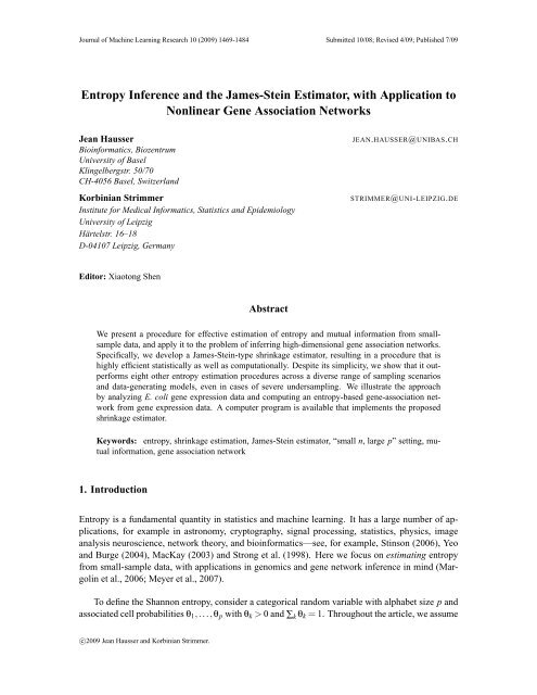
Figure 2: Left: Distribution of estimated mutual information values for all 5151 gene pairs of <strong>the</strong><br />
E. coli data set. Right: Mutual information values after applying <strong>the</strong> ARACNE gene<br />
pair selection procedure. Note that <strong>the</strong> most MIs have been set <strong>to</strong> zero by <strong>the</strong> ARACNE<br />
algorithm.<br />
For illustration, we now analyze data from Schmidt-Heck et al. (2004) who conducted an experiment<br />
<strong>to</strong> observe <strong>the</strong> stress response in E. Coli during expression of a recombinant protein. This<br />
1477
HAUSSER AND STRIMMER<br />
data set was also used in previous linear network analyzes, for example, in Schäfer <strong>and</strong> Strimmer<br />
(2005b). The raw data consist of 4289 protein coding genes, on which measurements were taken<br />
at 0, 8, 15, 22, 45, 68, 90, 150, <strong>and</strong> 180 minutes. We focus on a subset of G = 102 differentially<br />
expressed genes as given in Schmidt-Heck et al. (2004).<br />
Discretization of <strong>the</strong> data according <strong>to</strong> Freedman <strong>and</strong> Diaconis (1981) yielded K = 16 distinct<br />
gene expression levels. From <strong>the</strong> G = 102 genes, we estimated MIs for 5151 pairs of genes. For each<br />
pair, <strong>the</strong> mutual information was based on an estimated 16 × 16 contingency table, hence p = 256.<br />
As <strong>the</strong> number of time points is n = 9, this is a strongly undersampled situation which requires <strong>the</strong><br />
use of a regularized estimate of entropy <strong>and</strong> mutual information.<br />
The distribution of <strong>the</strong> shrinkage estimates of mutual information for all 5151 gene pairs is<br />
shown in <strong>the</strong> left side of Figure 2. The right h<strong>and</strong> side depicts <strong>the</strong> distribution of mutual information<br />
values after applying <strong>the</strong> ARACNE procedure, which yields 112 gene pairs <strong>with</strong> nonzero MIs.<br />
The model selection provided by ARACNE is based on applying <strong>the</strong> information processing<br />
inequality <strong>to</strong> all gene triplets. For each triplet, <strong>the</strong> gene pair corresponding <strong>to</strong> <strong>the</strong> smallest MI is discarded,<br />
which has <strong>the</strong> effect <strong>to</strong> remove gene-gene links that correspond <strong>to</strong> indirect ra<strong>the</strong>r than direct<br />
interactions. This is similar <strong>to</strong> a procedure used in graphical Gaussian models where correlations<br />
are transformed in<strong>to</strong> partial correlations. Thus, both <strong>the</strong> ARACNE <strong>and</strong> <strong>the</strong> MRNET algorithms can<br />
be considered as devices <strong>to</strong> approximate <strong>the</strong> conditional mutual information (Meyer et al., 2007).<br />
As a result, <strong>the</strong> 112 nonzero MIs recovered by <strong>the</strong> ARACNE algorithm correspond <strong>to</strong> statistically<br />
detectable direct associations.<br />
The corresponding gene association network is depicted in Figure 3. The most striking feature<br />
of <strong>the</strong> graph are <strong>the</strong> “hubs” belonging <strong>to</strong> genes hupB, sucA <strong>and</strong> nuoL. hupB is a well known DNAbinding<br />
transcriptional regula<strong>to</strong>r, whereas both nuoL <strong>and</strong> sucA are key components of <strong>the</strong> E. coli<br />
metabolism. Note that a Lasso-type procedure (that implicitly limits <strong>the</strong> number of edges that can<br />
connect <strong>to</strong> each node) such as that of Meinshausen <strong>and</strong> Bühlmann (2006) cannot recover <strong>the</strong>se hubs.<br />
6. Discussion<br />
We proposed a <strong>James</strong>-<strong>Stein</strong>-type shrinkage estima<strong>to</strong>r for inferring entropy <strong>and</strong> mutual information<br />
from small samples. While this is a challenging problem, we showed that our approach is highly<br />
efficient both statistically <strong>and</strong> computationally despite its simplicity.<br />
In terms of versatility, our estima<strong>to</strong>r has two distinct advantages over <strong>the</strong> NSB <strong>and</strong> Chao-Shen<br />
estima<strong>to</strong>rs. First, in addition <strong>to</strong> estimating <strong>the</strong> entropy, it also provides <strong>the</strong> underlying multinomial<br />
frequencies for use <strong>with</strong> <strong>the</strong> Shannon formula (Equation 1). This is useful in <strong>the</strong> context of using<br />
mutual information <strong>to</strong> quantify non-linear pairwise dependencies for instance. Second, unlike NSB,<br />
it is a fully analytic estima<strong>to</strong>r.<br />
Hence, our estima<strong>to</strong>r suggests itself for applications in large scale estimation problems. To<br />
demonstrate its application in <strong>the</strong> context of genomics <strong>and</strong> systems biology, we have estimated an<br />
entropy-based gene dependency network from expression data in E. coli. This type of approach may<br />
prove helpful <strong>to</strong> overcome <strong>the</strong> limitations of linear models currently used in network analysis.<br />
In short, we believe <strong>the</strong> proposed small-sample entropy estima<strong>to</strong>r will be a valuable contribution<br />
<strong>to</strong> <strong>the</strong> growing <strong>to</strong>olbox of machine learning <strong>and</strong> statistics procedures for high-dimensional data<br />
analysis.<br />
1478
ENTROPY INFERENCE AND THE JAMES-STEIN ESTIMATOR<br />
<br />
<br />
<br />
<br />
<br />
<br />
<br />
<br />
<br />
<br />
<br />
<br />
<br />
<br />
<br />
<br />
<br />
<br />
<br />
<br />
<br />
<br />
<br />
<br />
<br />
<br />
<br />
<br />
<br />
<br />
<br />
<br />
<br />
<br />
<br />
<br />
<br />
<br />
<br />
<br />
<br />
<br />
<br />
<br />
<br />
<br />
<br />
<br />
<br />
<br />
<br />
<br />
<br />
<br />
<br />
<br />
<br />
<br />
<br />
<br />
<br />
<br />
<br />
<br />
<br />
<br />
<br />
<br />
<br />
<br />
<br />
<br />
<br />
<br />
<br />
<br />
<br />
<br />
<br />
<br />
<br />
<br />
<br />
<br />
<br />
<br />
<br />
<br />
<br />
<br />
<br />
<br />
<br />
<br />
<br />
<br />
<br />
<br />
<br />
<br />
<br />
<br />
Figure 3: Mutual information network for <strong>the</strong> E. coli data inferred by <strong>the</strong> ARACNE algorithm based<br />
on shrinkage estimates of entropy <strong>and</strong> mutual information.<br />
1479
HAUSSER AND STRIMMER<br />
Acknowledgments<br />
This work was partially supported by a Emmy Noe<strong>the</strong>r grant of <strong>the</strong> Deutsche Forschungsgemeinschaft<br />
(<strong>to</strong> K.S.). We thank <strong>the</strong> anonymous referees <strong>and</strong> <strong>the</strong> edi<strong>to</strong>r for very helpful comments.<br />
Appendix A. Recipe For Constructing <strong>James</strong>-<strong>Stein</strong>-type Shrinkage <strong>Estima<strong>to</strong>r</strong>s<br />
The original <strong>James</strong>-<strong>Stein</strong> estima<strong>to</strong>r (<strong>James</strong> <strong>and</strong> <strong>Stein</strong>, 1961) was proposed <strong>to</strong> estimate <strong>the</strong> mean of<br />
a multivariate normal distribution from a single (n = 1!) vec<strong>to</strong>r observation. Specifically, if x is a<br />
sample from N p (µ,I) <strong>the</strong>n <strong>James</strong>-<strong>Stein</strong> estima<strong>to</strong>r is given by<br />
ˆµ JS<br />
k = (1 − p − 2<br />
∑ p )x k .<br />
k=1 x2 k<br />
Intriguingly, this estima<strong>to</strong>r outperforms <strong>the</strong> maximum likelihood estima<strong>to</strong>r ˆµ ML<br />
k<br />
= x k in terms of<br />
mean squared error if <strong>the</strong> dimension is p ≥ 3. Hence, <strong>the</strong> <strong>James</strong>-<strong>Stein</strong> estima<strong>to</strong>r dominates <strong>the</strong><br />
maximum likelihood estima<strong>to</strong>r.<br />
The above estima<strong>to</strong>r can be slightly generalized by shrinking <strong>to</strong>wards <strong>the</strong> component average<br />
¯x = ∑ p k=1 x k ra<strong>the</strong>r than <strong>to</strong> zero, resulting in<br />
<strong>with</strong> estimated shrinkage intensity<br />
ˆµ Shrink<br />
k<br />
ˆλ ⋆ =<br />
= ˆλ ⋆ ¯x+(1 − ˆλ ⋆ )x k<br />
p − 3<br />
∑ p k=1 (x k − ¯x) 2.<br />
The <strong>James</strong>-<strong>Stein</strong> shrinkage principle is very general <strong>and</strong> can be put <strong>to</strong> <strong>to</strong> use in many o<strong>the</strong>r<br />
high-dimensional settings. In <strong>the</strong> following we summarize a simple recipe for constructing <strong>James</strong>-<br />
<strong>Stein</strong>-type shrinkage estima<strong>to</strong>rs along <strong>the</strong> lines of Schäfer <strong>and</strong> Strimmer (2005b) <strong>and</strong> Opgen-Rhein<br />
<strong>and</strong> Strimmer (2007a).<br />
In short, <strong>the</strong>re are two key ideas at work in <strong>James</strong>-<strong>Stein</strong> shrinkage:<br />
i) regularization of a high-dimensional estima<strong>to</strong>r ˆθ by linear combination <strong>with</strong> a lowerdimensional<br />
target estimate ˆθ Target , <strong>and</strong><br />
ii) adaptive estimation of <strong>the</strong> shrinkage parameter λ from <strong>the</strong> data by quadratic risk minimization.<br />
A general form of a <strong>James</strong>-<strong>Stein</strong>-type shrinkage estima<strong>to</strong>r is given by<br />
ˆθ Shrink = λˆθ Target +(1 − λ)ˆθ. (9)<br />
Note that ˆθ <strong>and</strong> ˆθ Target are two very different estima<strong>to</strong>rs (for <strong>the</strong> same underlying model!). ˆθ as a<br />
high-dimensional estimate <strong>with</strong> many independent components has low bias but for small samples<br />
a potentially large variance. In contrast, <strong>the</strong> target estimate ˆθ Target is low-dimensional <strong>and</strong> <strong>the</strong>refore<br />
is generally less variable than ˆθ but at <strong>the</strong> same time is also more biased. The <strong>James</strong>-<strong>Stein</strong> estimate<br />
1480
ENTROPY INFERENCE AND THE JAMES-STEIN ESTIMATOR<br />
is a weighted average of <strong>the</strong>se two estima<strong>to</strong>rs, where <strong>the</strong> weight is chosen in a data-driven fashion<br />
such that ˆθ Shrink is improved in terms of mean squared error relative <strong>to</strong> both ˆθ <strong>and</strong> ˆθ Target .<br />
A key advantage of <strong>James</strong>-<strong>Stein</strong>-type shrinkage is that <strong>the</strong> optimal shrinkage intensity λ ⋆ can be<br />
calculated analytically <strong>and</strong> <strong>with</strong>out knowing <strong>the</strong> true value θ, via<br />
λ ⋆ = ∑p k=1 Var(ˆθ k ) − Cov(ˆθ k , ˆθ Target<br />
k<br />
)+Bias(ˆθ k )E(ˆθ k − ˆθ Target<br />
∑ p k=1 E[(ˆθ k − ˆθ Target<br />
k<br />
) 2 ]<br />
k<br />
)<br />
. (10)<br />
A simple estimate of λ ⋆ is obtained by replacing all variances <strong>and</strong> covariances in Equation 10 <strong>with</strong><br />
<strong>the</strong>ir empirical counterparts, followed by truncation of ˆλ ⋆ at 1 (so that ˆλ ⋆ ≤ 1 always holds).<br />
Equation 10 is discussed in detail in Schäfer <strong>and</strong> Strimmer (2005b) <strong>and</strong> Opgen-Rhein <strong>and</strong> Strimmer<br />
(2007a). More specialized versions of it are treated, for example, in Ledoit <strong>and</strong> Wolf (2003) for<br />
unbiased ˆθ <strong>and</strong> in Thompson (1968) (unbiased, univariate case <strong>with</strong> deterministic target). A very<br />
early version (univariate <strong>with</strong> zero target) even predates <strong>the</strong> estima<strong>to</strong>r of <strong>James</strong> <strong>and</strong> <strong>Stein</strong>, see Goodman<br />
(1953). For <strong>the</strong> multinormal setting of <strong>James</strong> <strong>and</strong> <strong>Stein</strong> (1961), Equation 9 <strong>and</strong> Equation 10<br />
reduce <strong>to</strong> <strong>the</strong> shrinkage estima<strong>to</strong>r described in Stigler (1990).<br />
<strong>James</strong>-<strong>Stein</strong> shrinkage has an empirical Bayes interpretation (Efron <strong>and</strong> Morris, 1973). Note,<br />
however, that only <strong>the</strong> first two moments of <strong>the</strong> distributions of ˆθ Target <strong>and</strong> ˆθ need <strong>to</strong> be specified in<br />
Equation 10. Hence, <strong>James</strong>-<strong>Stein</strong> estimation may be viewed as a quasi-empirical Bayes approach<br />
(in <strong>the</strong> same sense as in quasi-likelihood, which also requires only <strong>the</strong> first two moments).<br />
Appendix B. Computer Implementation<br />
The proposed shrinkage estima<strong>to</strong>rs of entropy <strong>and</strong> mutual information, as well as all o<strong>the</strong>r investigated<br />
entropy estima<strong>to</strong>rs, have been implemented in R (R Development Core Team, 2008). A<br />
corresponding R package “entropy” was deposited in <strong>the</strong> R archive CRAN <strong>and</strong> is accessible at <strong>the</strong><br />
URL http://cran.r-project.org/web/packages/entropy/ under <strong>the</strong> GNU General Public<br />
License.<br />
References<br />
A. Agresti <strong>and</strong> D. B. Hitchcock. Bayesian inference for categorical data analysis. Statist. Meth.<br />
Appl., 14:297–330, 2005.<br />
A. J. Butte, P. Tamayo, D. Slonim, T. R. Golub, <strong>and</strong> I. S. Kohane. Discovering functional relationships<br />
between RNA expression <strong>and</strong> chemo<strong>the</strong>rapeutic susceptibility using relevance networks.<br />
Proc. Natl. Acad. Sci. USA, 97:12182–12186, 2000.<br />
A. Chao <strong>and</strong> T.-J. Shen. Nonparametric estimation of Shannon’s index of diversity when <strong>the</strong>re are<br />
unseen species. Environ. Ecol. Stat., 10:429–443, 2003.<br />
A. Dobra, C. Hans, B. Jones, J. R. Nevins, G. Yao, <strong>and</strong> M. West. Sparse graphical models for<br />
exploring gene expression data. J. Multiv. Anal., 90:196–212, 2004.<br />
B. Efron <strong>and</strong> C. N. Morris. <strong>Stein</strong>’s estimation rule <strong>and</strong> its competi<strong>to</strong>rs–an empirical Bayes approach.<br />
J. Amer. Statist. Assoc., 68:117–130, 1973.<br />
1481
HAUSSER AND STRIMMER<br />
S. E. Fienberg <strong>and</strong> P. W. Holl<strong>and</strong>. Simultaneous estimation of multinomial cell probabilities. J.<br />
Amer. Statist. Assoc., 68:683–691, 1973.<br />
D. Freedman <strong>and</strong> P. Diaconis. On <strong>the</strong> his<strong>to</strong>gram as a density estima<strong>to</strong>r: L2 <strong>the</strong>ory. Z. Wahrscheinlichkeits<strong>the</strong>orie<br />
verw. Gebiete, 57:453–476, 1981.<br />
N. Friedman. Inferring cellular networks using probabilistic graphical models. Science, 303:799–<br />
805, 2004.<br />
S. Geisser. On prior distributions for binary trials. The American Statistician, 38:244–251, 1984.<br />
A. Gelman, J. B. Carlin, H. S. Stern, <strong>and</strong> D. B. Rubin. Bayesian Data Analysis. Chapman &<br />
Hall/CRC, Boca Ra<strong>to</strong>n, 2nd edition, 2004.<br />
I. J. Good. The population frequencies of species <strong>and</strong> <strong>the</strong> estimation of population parameters.<br />
Biometrika, 40:237–264, 1953.<br />
L. A. Goodman. A simple method for improving some estima<strong>to</strong>rs. Ann. Math. Statist., 24:114–117,<br />
1953.<br />
M. H. J. Gruber. Improving Efficiency By Shrinkage. Marcel Dekker, Inc., New York, 1998.<br />
D. Holste, I. Große, <strong>and</strong> H. Herzel. Bayes’ estima<strong>to</strong>rs of generalized entropies. J. Phys. A: Math.<br />
Gen., 31:2551–2566, 1998.<br />
D. G. Horvitz <strong>and</strong> D. J. Thompson. A generalization of sampling <strong>with</strong>out replacement from a finite<br />
universe. J. Amer. Statist. Assoc., 47:663–685, 1952.<br />
W. <strong>James</strong> <strong>and</strong> C. <strong>Stein</strong>. Estimation <strong>with</strong> quadratic loss. In Proc. Fourth Berkeley Symp. Math.<br />
Statist. Probab., volume 1, pages 361–379, Berkeley, 1961. Univ. California Press.<br />
H. Jeffreys. An invariant form for <strong>the</strong> prior probability in estimation problems. Proc. Roc. Soc.<br />
(Lond.) A, 186:453–461, 1946.<br />
M. Kalisch <strong>and</strong> P. Bühlmann. Estimating high-dimensional directed acyclic graphs <strong>with</strong> <strong>the</strong> PCalgorithm.<br />
J. Machine Learn. Res., 8:613–636, 2007.<br />
R. E. Krichevsky <strong>and</strong> V. K. Trofimov. The performance of universal encoding. IEEE Trans. Inf.<br />
Theory, 27:199–207, 1981.<br />
H. Lähdesmäki <strong>and</strong> I. Shmulevich. Learning <strong>the</strong> structure of dynamic Bayesian networks from time<br />
series <strong>and</strong> steady state measurements. Mach. Learn., 71:185–217, 2008.<br />
O. Ledoit <strong>and</strong> M. Wolf. Improved estimation of <strong>the</strong> covariance matrix of s<strong>to</strong>ck returns <strong>with</strong> an<br />
application <strong>to</strong> portfolio selection. J. Empir. Finance, 10:603–621, 2003.<br />
D. J. C. MacKay. Information Theory, <strong>Inference</strong>, <strong>and</strong> Learning Algorithms. Cambridge University<br />
Press, Cambridge, 2003.<br />
A.A. Margolin, I. Nemenman, K. Basso, C. Wiggins, G. S<strong>to</strong>lovitzky, R. Dalla Favera, <strong>and</strong> A. Califano.<br />
ARACNE: an algorithm for <strong>the</strong> reconstruction of gene regula<strong>to</strong>ry networks in a mammalian<br />
cellular context. BMC Bioinformatics, 7 (Suppl. 1):S7, 2006.<br />
1482
ENTROPY INFERENCE AND THE JAMES-STEIN ESTIMATOR<br />
N. Meinshausen <strong>and</strong> P. Bühlmann. High-dimensional graphs <strong>and</strong> variable selection <strong>with</strong> <strong>the</strong> Lasso.<br />
Ann. Statist., 34:1436–1462, 2006.<br />
P. E. Meyer, K. Kon<strong>to</strong>s, F. Lafitte, <strong>and</strong> G. Bontempi. Information-<strong>the</strong>oretic inference of large transcriptional<br />
regula<strong>to</strong>ry networks. EURASIP J. Bioinf. Sys. Biol., page doi:10.1155/2007/79879,<br />
2007.<br />
G. A. Miller. Note on <strong>the</strong> bias of information estimates. In H. Quastler, edi<strong>to</strong>r, Information Theory<br />
in Psychology II-B, pages 95–100. Free Press, Glencoe, IL, 1955.<br />
I. Nemenman, F. Shafee, <strong>and</strong> W. Bialek. <strong>Entropy</strong> <strong>and</strong> inference, revisited. In T. G. Dietterich,<br />
S. Becker, <strong>and</strong> Z. Ghahramani, edi<strong>to</strong>rs, Advances in Neural Information Processing Systems 14,<br />
pages 471–478, Cambridge, MA, 2002. MIT Press.<br />
R. Opgen-Rhein <strong>and</strong> K. Strimmer. Accurate ranking of differentially expressed genes by a<br />
distribution-free shrinkage approach. Statist. Appl. Genet. Mol. Biol., 6:9, 2007a.<br />
R. Opgen-Rhein <strong>and</strong> K. Strimmer. From correlation <strong>to</strong> causation networks: a simple approximate<br />
learning algorithm <strong>and</strong> its application <strong>to</strong> high-dimensional plant gene expression data. BMC<br />
Systems Biology, 1:37, 2007b.<br />
A. Orlitsky, N. P. Santhanam, <strong>and</strong> J. Zhang. Always Good Turing: asymp<strong>to</strong>tically optimal probability<br />
estimation. Science, 302:427–431, 2003.<br />
W. Perks. Some observations on inverse probability including a new indifference rule. J. Inst.<br />
Actuaries, 73:285–334, 1947.<br />
R Development Core Team. R: A Language <strong>and</strong> Environment for Statistical Computing. R Foundation<br />
for Statistical Computing, Vienna, Austria, 2008. URL http://www.R-project.org.<br />
ISBN 3-900051-07-0.<br />
C. Rangel, J. Angus, Z. Ghahramani, M. Lioumi, E. So<strong>the</strong>ran, A. Gaiba, D. L. Wild, <strong>and</strong> F. Falciani.<br />
Modeling T-cell activation using gene expression profiling <strong>and</strong> state space modeling. Bioinformatics,<br />
20:1361–1372, 2004.<br />
J. Schäfer <strong>and</strong> K. Strimmer. An empirical Bayes approach <strong>to</strong> inferring large-scale gene association<br />
networks. Bioinformatics, 21:754–764, 2005a.<br />
J. Schäfer <strong>and</strong> K. Strimmer. A shrinkage approach <strong>to</strong> large-scale covariance matrix estimation <strong>and</strong><br />
implications for functional genomics. Statist. Appl. Genet. Mol. Biol., 4:32, 2005b.<br />
W. Schmidt-Heck, R. Guthke, S. Toepfer, H. Reischer, K. Duerrschmid, <strong>and</strong> K. Bayer. Reverse<br />
engineering of <strong>the</strong> stress response during expression of a recombinant protein. In Proceedings<br />
of <strong>the</strong> EUNITE symposium, 10-12 June 2004, Aachen, Germany, pages 407–412, 2004. Verlag<br />
Mainz.<br />
T. Schürmann <strong>and</strong> P. Grassberger. <strong>Entropy</strong> estimation of symbol sequences. Chaos, 6:414–427,<br />
1996.<br />
S. M. Stigler. A Gal<strong>to</strong>nian perspective on shrinkage estima<strong>to</strong>rs. Statistical Science, 5:147–155,<br />
1990.<br />
1483
HAUSSER AND STRIMMER<br />
D.R. Stinson. Cryp<strong>to</strong>graphy: Theory <strong>and</strong> Practice. CRC Press, 2006.<br />
S. P. Strong, R. Koberle, R. de Ruyter van Steveninck, <strong>and</strong> W. Bialek. <strong>Entropy</strong> <strong>and</strong> information in<br />
neural spike trains. Phys. Rev. Letters, 80:197–200, 1998.<br />
J. R. Thompson. Some shrinkage techniques for estimating <strong>the</strong> mean. J. Amer. Statist. Assoc., 63:<br />
113–122, 1968.<br />
S. Trybula. Some problems of simultaneous minimax estimation. Ann. Math. Statist., 29:245–253,<br />
1958.<br />
F. Tuyl, R. Gerlach, <strong>and</strong> K. Mengersen. A comparison of Bayes-Laplace, Jeffreys, <strong>and</strong> o<strong>the</strong>r priors:<br />
<strong>the</strong> case of zero events. The American Statistician, 62:40–44, 2008.<br />
V. Q. Vu, B. Yu, <strong>and</strong> R. E. Kass. Coverage-adjusted entropy estimation. Stat. Med., 26:4039–4060,<br />
2007.<br />
G. Yeo <strong>and</strong> C. B. Burge. Maximum entropy modeling of short sequence motifs <strong>with</strong> applications <strong>to</strong><br />
RNA splicing signals. J. Comp. Biol., 11:377–394, 2004.<br />
1484