Competitive Learning Algorithm of Neural Network - International ...

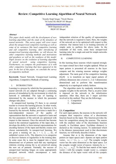
Jitendra Singh Sengar et al, Int. J. Comp. Tech. Appl., Vol 2 (5), 1480-1485 

ISSN:2229-6093 

Review: Competitive Learning Algorithm of Neural Network 

1 Jitendra Singh Sengar, 2 Niresh Sharma 

1 M.Tech(CSE) RKDF IST Bhopal 

jitendrasingsengar@gmail.com 

2 HOD Department of CSE 

RKDF IST Bhopal 

Abstract 

This paper deals mainly with the development of new 

learning algorithms and the study of the dynamics of 

neural networks. This survey paper will cover issues 

about the unsupervised competitive learning as well as 

some of its variances like hard competitive learning 

and soft competitive learning. After introducing of 

unsupervised learning algorithms, we will discuss the 

other competitive learning methods and motivations 

and goodness as well as the weakness of this model. 

Paper focuses on the evolution of learning algorithm 

of neural network using competitive learning, 

Furthermore, we compare the performance of it with 

other competitive learning that have appeared in the 

past. In the last of this paper, we conclude the survey 

of competitive methods 

Keywords: Neural Network, Unsupervised Learning 

Algorithms, Competitive Methods of learning. 

I. INTRODUCTION 

Learning is a process by which the free parameters of a 

neural network [3] are adapted through a continuing 

process of stimulation by the environment in which the 

network is embedded. The type of learning is 

determined by the manner in which the parameter 

changes take place. 

In unsupervised learning [7] there is no external 

teacher to oversee the learning process. In other words, 

there are no specific samples of the function to be 

learned by the network. Rather, provision is made for a 

task-independent measure of the quality of 

representation that the network is required to learn and 

the free parameters of the network are optimized with 

respect to that measure. Once the network has become 

tuned to the statistical regularities of the input data, it 

develops the ability to form internal representations for 

encoding features of the input and thereby creates new 

classes automatically. In unsupervised learning, We 

are given a training set {x i ; i = 1, 2, ..., m}, of 

unlabeled vectors in R n . The objective is to categorize 

or discover features or regularities in the training data. 

In some cases the x i must be mapped into a lower 

dimensional set of patterns such that any topological 

relations existing among the x i are preserved among 

the new set of patterns. Normally, the success of 

unsupervised learning hinges on some appropriately 

designed network which encompasses a taskindependent 

criterion of the quality of representation 

that the network is required to learn. Here, the weights 

of the network are to be optimized with respect to this 

criterion. Our interest here is in training networks of 

simple units to perform the above tasks. In the 

remainder of this work, some basic unsupervised 

learning rules for a single unit and for simple networks 

are introduced. 

II. 

COMPETITIVE LEARNING 

In this learning those neurons which respond strongly 

two input stimuli have their weights updated. When an 

input pattern is presented all neurons in the layer 

compete and the winning neurons undergo weights 

adjustment. The main goal of the competitive learning 

[6],[8] is to transform an input signal pattern of 

arbitrary dimension into a lower (1, 2 or 3 dimensions) 

dimensional and to perform this transformation 

adaptively in a topological orderly fashion. 

The algorithm starts by randomly initializing the 

synaptic weights in the network. That is, no prior order 

is imposed on the network in the initialization 

operation. After that, there are 3 major activities 

involved in this method. They are the followings: 

1. Competition 

2. Adjustment 

2.1. Competition 

For each input pattern, the neurons in the network will 

compute their respective values of a discriminate 

function based on the input. This function provides the 

basis for competition among the neurons. The neuron 

with the smallest value of the discriminate function 

(usually in Euclidean space: Euclidean distance) is 

declared as the winning neuron. To understand which 

is the distance measurement used in that discriminate 

function, we will briefly describe it below. 

Assume that m is the dimension of the input 

pattern (or input space) and v denotes an input pattern 

vector., i.e. v = [v 1 , v 2 , …, v m ] T . The synaptic weight 

vector has the same dimension as the input space. Let 

the synaptic weight vector of neuron i denotes by w i = 

[w i1 , w i2 , …, w im ] T . To find the best match of the input 

vector v with the synaptic weight vector w i , compare 

the distance of the input vector with all the synaptic 

IJCTA | SEPT-OCT 2011 

Available online@www.ijcta.com 

1480

weight vectors for i = 1, … N, where N is the total 

number of neurons, and select the smallest. The 

selection of the best matching or winning neuron k as, 

k arg min v w , where i 1,..., N 


i 

i 

2 

dik 

hik 

, 

2 

2 

n 

( n) 

 

0 

exp 

, n 01 , , 2, 

3 

τ 

 

1 

2.2. Adjustment 

The winning neuron k determines the spatial location 

of a topological neighborhood of excited neurons, i.e. 

determines all the neurons that in the “neighborhood 

area” of the winning neuron. According to 

neurobiological evidence (lateral inhibition or some 

times called on-center-off-surround), a neuron that is 

firing tends to excite the neurons in its neighborhood 

more than those far away from it. This observation 

leads the competitive learning algorithm to define the 

topological neighborhood around the winning neuron k 

as explained below. 

Let d ik be the lateral distance between the winning 

neuron k and the excited neuron i. We can define the 

topological neighborhood h ik as a uni-modal function 

with the following two requirements: 

1) It is symmetric about the maximum point defined 

by d ik = 0. 

2) Its amplitude decreases monotonically to zero with 

increasing lateral distance d ik . A typical choice of 

h ik that satisfies this requirement is the Gaussian 

function: 

where δ is the width of the topological neighborhood. 

The δ reduction scheme ensures that the map actually 

approaches a neighborhood preserving the final 

structure, assumed that such a structure exists. If the 

topology of the output space does not match that of the 

data manifold, neighborhood violations is inevitable. 

An example of such a reduction scheme is provide 

below: 

 

 

where n indicates the number of sequence, δ 0 is the 

beginning value of δ, and τ l is the time parameter used 

to reduce the value of the width of the topological 

neighborhood. Or another simple method used to 

decrease the δ is just multiple it by a value that is less 

than 1, say, 0.9. These two methods are similar to the 

simulated annealing scheme with the following note: 

The spread of the neighborhood function should 

initially include all neurons for any winning neuron 

and during the ordering phase should be slowly 

reduced to eventually include only a few neurons in 

the winner’s neighborhood. During the convergence 

phase, the neighborhood function should include only 

the winning neuron. 

For the network to be self-organizing, the 

synaptic weight vector w i of neuron i is required to 

change in relation to the input vector v. This is a kind 

of un-supervised learning, so we can use a modified 

version of Hebbian learning [1] by including a 

forgetting term g(y i ) that is used to keep the weight 

from growing large, where g(y i ) is some positive scalar 

function of the response of the network y i . So, we can 

define the change to the weight vector as: 

Δw i = ηy i v – g(y i )w i , 

where η is the learning rate. Furthermore, we can 

define g(y i ) as a linear function of y i , say, g(y i ) = ηy i 

and setting y i = h ik . So we can simplify above equation 

to the following: 

Δw i = ηh ik (v – w i ). 

Using discrete time formalism, we can derive the 

final formula for the weight update procedure: 

w i (n+1) = w i (n) +η(n) h ik (n) [v(n) – w i (n)], 

Where n denotes the times step updating the 

weight. This above equation will be applied to all the 

neurons that lie inside the neighborhood of the 

winning neuron (other neurons are also updated but the 

weight change is zero caused by the value of the 

neighborhood function). Upon repeated presenting 

training data, the synaptic weight tends to follow the 

distribution of the input data due to neighborhood 

updating, which causes the adaptation of the weight 

vectors to the input. The neighborhood updating also 

makes the weights between neighbor neurons have the 

similar values to each other. 

a. Simple Competitive Learning 

ISSN:2229-6093 

Figure 2: A sample reduction scheme of δ 

Because we are now dealing with competition, it only 

makes sense to consider a group of interacting units. 

We assume the simplest architecture where we have a 

single layer of units, each receiving the same input x 



1481


ISSN:2229-6093 

Rn and producing an output yi. We also assume that 

only one unit is active at a given time. This active unit 

is called the "winner" and is determined as the unit 

with the largest weighted-sum net i k ,. 

where 

…………. (1) 

and x k is the current input. Thus, unit i is the winning 

unit if 

which may be written as 

….. (2) 

….. (3) 

if |w i |=1for all i = 1, 2, ..., m. Thus, the winner is the 

node with the weight vector closest (in a Euclidean 

distance sense) to the input vector. It is interesting to 

note that lateral inhibition may be employed here in 

order to implement the "winner-take-all" operation in 

Equation (2) or (3). This is similar to what we have 

described in the previous section with a slight 

variation: Each unit inhibits all other units and selfexcites 

itself, as shown in Figure 1. 

Lippmann, 1987). One possible choice for the lateral 

weights is 

………… (4) 

where 0 < < and m is the number of units in the 

network. An appropriate activation function for this 

type of network is shown in figure, where T is chosen 

such that the outputs y i do not saturate at 1 before 

convergence of the winner-take-all competition; after 

convergence, only the winning unit will saturate at 1 

with all other units having zero outputs. Note, 

however, that if one is training the net as part of a 

computer simulation, there is no need for the winnertake-all 

net to be implemented explicitly; it is more 

efficient from a computation point of view to perform 

the winner selection by direct search for the maximum 

neti. Thus far, we have only described the competition 

mechanism of the competitive learning technique[2]. 

Next, we give a learning equation for weight 

updating. For a given input x k drawn from a random 

distribution p(x), the weights of the winning unit are 

updated (the weights of all other units are left 

unchanged) according to (Grossberg, 1969; von der 

Malsburg, 1973; Rumelhart and Zipser, 1985): 

………..(5) 

If the magnitudes of the input vectors contain no useful 

information, a more appropriate rule to use is 

…………. (6) 

Figure 

In order to assure winner-take-all operation, a proper 

choice of lateral weights and unit activation functions 

must be made (e.g., see Grossberg, 1976, and 

The above rules tend to tilt the weight vector of the 

current winning unit in the direction of the current 

input. The cumulative effect of the repetitive 

application of the above rules can be described as 

follows. Let us view the input and weight vectors as 

points scattered on the surface of a hypersphere. The 

effect of the application of the competitive learning 



1482


ISSN:2229-6093 

rule is to sensitize certain units towards neighboring 

clusters of input data. Ultimately, some units (frequent 

winner units) will evolve so that their weight vector 

points towards the "center of mass" of the nearest 

significant dense cluster of data points. 

b. Learning Vector Quantization 

One of the common applications of competitive 

learning is adaptive vector quantization [4] for data 

compression (e.g., speech and image data). Here, we 

need to categorize a given set of x k data points 

(vectors) into m "templates" so that later one may use 

an encoded version of the corresponding template of 

any input vector to represent the vector, as opposed to 

using the vector itself. This leads to efficient 

quantization (compression) for storage and for 

transmission purposes (albeit at the expense of some 

distortion). Vector quantization is a technique whereby 

the input space is divided into a number of distinct 

regions, and for each region a "template" 

(reconstruction vector) is defined. When presented 

with a new input vector x, a vector quantizer first 

determines the region in which the vector lies. Then, 

the quantizer outputs an encoded version of the 

reconstruction vector w i representing that particular 

region containing x. The set of all possible 

reconstruction vectors w i is usually called the 

"codebook" of the quantizer. 

When the Euclidean distance similarity measure is 

used to decide on the region to which the input x 

belongs, the quantizer is called Voronoi quantizer. The 

Voronoi quantizer partitions its input space into 

Voronoi cells, each cell is represented by one of the 

reconstruction vectors, w i . The ith Voronoi cell 

contains those points of the input space that are closest 

(in a Euclidean sense) to the vector w i than to any 

other vector w j , j i. The competitive learning rule with 

a winning unit determination based on the Euclidean 

distance may now be used in order to allocate a set of 

m reconstruction vectors , i = 1, 2, ..., m, to 

the input space of n-dimensional vectors x. Let x be 

distributed according to the probability density 

function p(x). Initially, we set the starting values of the 

vectors wi to the first m randomly generated samples 

of x. Additional samples x are then used for training. 

Here, the learning rate is selected as a monotonically 

decreasing function of the number of iterations k. 

Based on empirical results, Kohonen (1989) 

conjectured that, in an average sense, the asymptotic 

local point density of the w i (i.e., the number of w i 

falling in a small volume of R n centered at x) obtained 

by the above competitive learning process takes the 

form of a continuous, monotonically increasing 

function of p(x). Thus, this competitive learning 

algorithm may be viewed as an "approximate" method 

for computing the reconstruction vectors w i in an 

unsupervised manner. Kohonen (1989) designed 

supervised versions of vector quantization (called 

learning vector quantization, LVQ) for adaptive 

pattern classification. Here, class information is used 

to fine tune the reconstruction vectors in a Voronoi 

quantizer, so as to improve the quality of the classifier 

decision regions. In pattern classification problems, it 

is the decision surface between pattern classes and not 

the inside of the class distribution, which should be 

described most accurately. 

The above quantizer process can be easily adapted 

in order to optimize the placement of the decision 

surface between different classes. Here, one would 

start with a trained Voronoi quantizer and calibrate it 

using a set of labeled input samples (vectors). Each 

calibration sample is assigned to that w i which is 

closest. Each w i is then labeled according to the 

majority of classes represented among those samples 

which have been assigned to w i . Here, the distribution 

of the calibration samples to the various classes, as 

well as the relative numbers of the w i assigned to these 

classes must comply with the a piori probabilities of 

the classes, if such probabilities are known. Next, the 

tuning of the decision surfaces is accomplished by 

rewarding correct classifications and punishing 

incorrect ones. Let the training vector x k belong to the 

class c j . Assume that the closest reconstruction vector 

w i to x k carries the label of class c l . Then, only vector 

w i is updated according to the following supervised 

rule (LVQ rule): 

(7) 

where k is assumed to be a monotonically decreasing 

function of the number of iterations k. After 

convergence, the input space R n is again partitioned by 

a Voronoi tessellation corresponding to the tuned w i 

vectors. The primary effect of the reward/punish rule 

in Equation (7) is to minimize the number of 



1483


ISSN:2229-6093 

misclassifications. At the same time, however, the 

vectors w i are pulled away from the zones of class 

overlap where misclassifications persist. 

The convergence speed of LVQ can be improved if 

each vector wi has its own adaptive learning rate 

given by (8) 

This recursive rule causes i to decrease if w i 

classifies x k correctly. Otherwise, i increases. 

Equations (7) and (8) define what is known as an 

"optimized learning rate" LVQ (OLVQ). Another 

improved algorithm named LVQ2 has also been 

suggested by Kohonen et al. (1988) which approaches 

the performance predicted by Bayes decision theory 

(Duda and Hart, 1973). Some theoretical aspects of 

competitive learning are considered in the next 

chapter. More general competitive networks with 

stable categorization behavior have been proposed by 

Carpenter and Grossberg . 

III. 

CURRENT TREND AND 

OUTLOOK FOR THE 

FUTURE 

In machine learning, unsupervised learning refers to 

the problem of trying to find hidden structure in 

unlabeled data. Since the examples given to the learner 

are unlabeled, there is no error or reward signal to 

evaluate a potential solution. This distinguishes 

unsupervised learning from supervised learning and 

reinforcement learning. Unsupervised learning is 

closely related to the problem of density estimation in 

statistics. However unsupervised learning also 

encompasses many other techniques that seek to 

summarize and explain key features of the data. 

Approaches to unsupervised learning include: 

clustering (e.g., k-means, mixture models, k- 

nearest neighbors, hierarchical clustering), 

blind signal separation using feature extraction 

techniques for dimensionality reduction (e.g., 

Principal component analysis, Independent 

component analysis, Non-negative matrix 

factorization, Singular value decomposition). 

Among neural network models, the self-organizing 

map (SOM) and adaptive resonance theory (ART) are 

commonly used unsupervised learning algorithms [5]. 

The SOM is a topographic organization in which 

nearby locations in the map represent inputs with 

similar properties. SOM algorithm becomes more and 

more interesting in many fields such as: pattern 

recognition, clustering, and function approximation, 

data- and web-mining. This survey will cover issues 

about the SOFM its self as well as some of its 

variances like Neural Gas, Growing Neural Gas, 

Growing Cell Structures, etc and they are all the kind 

of unsupervised competitive learning algorithms. 

The ART model allows the number of clusters to 

vary with problem size and lets the user control the 

degree of similarity between members of the same 

clusters by means of a user-defined constant called the 

vigilance parameter. ART networks are also used for 

many pattern recognition tasks, such as automatic 

target recognition and seismic signal processing. 

Input 

Pattern 

Single layer 

Feedforward NN 

SOFM 

Output 

Pattern 

Competitive 

learning 

Recurrent NN 

ART 

Output 

Pattern 

In future, we will propose an approach of neural 

network for unsupervised learning based on 

competitive learning set of any input pattern in. In this 

approach single layer self-organizing map learning 

will be used with the recurrent features that represent 

problem solution space as NN state space, find weights 

and define node function and produce only one set of 

output values rather than a sequence of values from a 

given input. These networks are memory-less in the 

sense that their response to an input is independent. 

Recurrent, or feedback, networks are dynamic systems. 

When a new input pattern is presented, the neuron 

outputs are computed. Because of the feedback paths, 

the inputs to each neuron are then modified, which 

leads the network to enter a new state. Different 

network architectures require appropriate learning 

algorithms. 



1484


ISSN:2229-6093 

IV. 

CONCLUSION AND FUTURE WORK 

Finally, simple, single layer networks of multiple 

interconnected units are considered in the context of 

competitive learning, learning vector quantization, 

principal component analysis, and self-organizing 

feature maps. Simulations are also included which are 

designed to illustrate the powerful emerging 

computational properties of these simple networks and 

their application. It is demonstrated that local 

interactions in a competitive net can lead to global 

order. A case in point is the SOFM where simple 

incremental interactions among locally neighboring 

units lead to a global map which preserves the 

topology and density of the input data. 

This paper considers the use of learning vector 

quantization to model aspects of development 

including of the property of recurrent rules of learning 

for strengthening of synaptic efficacy of structure in 

the visual system in early life. 

Refference 

[1] Lo,J.T.-H.; “Unsupervised Hebbian learning by 

recurrent multilayer neural networks for temporal 

hierarchical pattern recognition” Information Sciences 

and Systems (CISS), 2010 44th Annual Conference on 

Digital Object Identifier: 10.1109/CISS.2010.5464925 

Publication Year: 2010 , Page(s): 1 – 6. 

Organizing Map”Industrial and Information Systems, 

2008. ICIIS 2008. IEEE Region 10 and the Third 

international Conference on 

Digital Object Identifier: 10.1109 / ICIINFS .2008. 

Publication Year: 2008 , Page(s): 1 - 5. 

[6]Kamimura,R.; “Controlled Competitive Learning: 

Extending Competitive Learning to Supervised 

Learning”Neural Networks, 2007. IJCNN 2007. 

International Joint Conference on 

Digital Object Identifier: 10.1109 / IJCNN. 2007 . 

4371225 Publication Year: 2007 , Page(s): 1767 – 

1773. 

[7]Daxin Tian; Yanheng Liu; Da Wei; 

Intelligent Control and Automation, 2006. WCICA 

2006. The Sixth World Congress on 

Volume:1 Digital Object Identifier: 10.1109 / WCICA 

.2006.1712893 Publication Year: 2006 , Page(s): 2886 

- 2890. 

[8]Sutton, G.G., III; Reggia, J.A.; Maisog, J.M.; 

“Competitive learning using competitive activation 

rules” Neural Networks, 1990., 1990 IJCNN 

International Joint Conference on 

Digital Object Identifier: 10.1109/IJCNN.1990.137728 

Publication Year: 1990 , Page(s): 285 – 291. 

[2] Tung-Shou Chen; Jeanne Chen; Yuan-Hung Kao; 

Bai-JiunTu; “A Novel Anti-Competitive Learning 

Neural Network Technique against Mining Knowledge 

from Databases”Software Engineering, 2009. WCSE 

'09. WRI World Congress on 

Volume:4DigitalObjectIdentifier: 10.1109 / WCSE . 

2009.345 Publication Year: 2009 , Page(s): 383 – 386. 

[3]Shou-weiLi; “Analysis of Contrasting Neural 

Network with Small-World Network” Future 

Information Technology and Management 

Engineering, 2008. FITME '08. International Seminar 

on Digital Object Identifier: 10.1109/FITME.2008.55 

Publication Year: 2008 , Page(s): 57 - 60 

[4] Esakkirajan, S.; Veerakumar, T.; Navaneethan, P.; 

“Adaptive vector quantization technique for retinal 

image compression” Computing , Communication and 

Networking, 2008. ICCCn 2008. International 

Conference on Digital ObjectIdentifier: 10.1109 / 

ICCCNET.2008.4787724 Publication Year: 2008 , 

Page(s): 1 - 4 . 

[5]Chaudhuri, A.; De, K.; Chatterjee, D.; “A Study of 

the Traveling Salesman Problem Using Fuzzy Self 



1485

Competitive Learning Algorithm of Neural Network - International ...

You also want an ePaper? Increase the reach of your titles

Delete template?

Save as template?