Relay Approach for tuning of PID controller - International Journal of ...

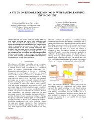
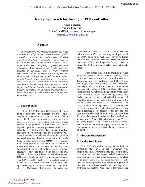
Amar G Khalore et al ,Int.J.Computer Technology & Applications,Vol 3 (3), 1237-1242 

ISSN:2229-6093 

Relay Approach for tuning of PID controller 

Amar g khalore 

Assistant professor 

Svkm’s NMIMS,mpstme,shirpur campus 

pappukhalore@gmail.com 

Abstract 

In recent years, relay feedback method has found 

a new lease of life in the automatic tuning of PID 

controllers and in the initialization of other 

sophisticated adaptive controllers. This tuner is 

based on the approximate estimation of the critical 

point on the process frequency response from relay 

oscillations. A continuous cycling of the controlled 

variable is generated from a relay feedback 

experiment and the important process information, 

ultimate gain and ultimate period can be extracted 

directly from the experiment. This is a very efficient 

way, i.e., a one shot solution, to generate sustained 

oscillations. The success of this auto tuner is due to 

the fact that the identification and tuning mechanism 

is simple so that process operators understand how it 

works. Moreover, it works well even in slow and nonlinear 

processes. 

1. “Introduction” 

The PID control algorithm remains the most 

popular approach for industrial process control 

despite continual advances in control theory. This is 

not only due to the simple structure which is 

conceptually easy to understand and which makes 

manual tuning possible but also to the fact that the 

algorithm provides adequate performance in the vast 

majority of applications. For many industrial 

problems, the proportional-integral derivative (PID) 

control module is a building block which provides 

the regulation and disturbance rejection for single 

loop, cascade multi loop and MIMO control system. 

It is widely used in process industries because of its 

simple structure and robustness to the modeling error. 

Sophisticated control algorithms, such as model 

predictive control are built on the basis of the PID 

algorithm. Even in non-linear control development, 

PID control has been used as comparison reference. 

The PID controller deals with important practical 

issues such as actuator saturation and integral wind 

up. According to a survey conducted by Japan 

electric Measuring Instruments Manufacturers 

Association in 1989, 90% of the control loops in 

industries are of PID type and only small portion of 

the control loop works well. Also survey by Ender 

indicates 30% of the controller is operated in manual 

mode and 20% of the loops use factory tuning. It 

means that PID controller is widely used but poorly 

tuned. 

Poor tuning can lead to mechanical wear 

associated with excessive control activity, poor 

control performance and even poor quality products. 

The present work is aimed to provide PID controller 

tuning guidelines using relay feedback approach. 

Recently much research effort has been focused on 

the automatic tuning of PID controllers, which was 

first proposed by Astrom and Hagglund (1984). They 

have introduced novel relay tuning method for 

finding the critical gain and critical frequency of 

closed loop process and proposed several tuning rules 

for PID controllers based on this information. The 

relay based PID tuning concept of Astrom and 

Hagglund is one of the simplest and most robust 

tuning techniques for process controllers and has 

been successfully applied to industry for more than 

15 years. Progresses in relay feedback method are 

summarized by Yu (1999) and Wang and Lee (2003). 

The relay feedback test is carried out under closedloop 

control so that with an appropriate choice of the 

relay parameters, the process can be kept close to the 

set point. 

2. “System description” 

2.1 Tuning techniques: 

The PID Controller tuning is method of 

computing the three control parameters viz. 

Proportional gain, Derivative time and Integral time, 

such that the controller meets desired performance 

specification. Since, the exact dynamics of the plant 

is generally unknown; the basic function of auto 

tuners is some experimental procedure through which 

plant information is obtained in order to compute the 

controller parameters. Auto tuning techniques can 

IJCTA | MAY-JUNE 2012 

Available online@www.ijcta.com 

1237


ISSN:2229-6093 

therefore be classified according to this experimental 

procedure. The Tuning methods can be broadly 

classified into the following categories where the 

classification is based on the availability of the 

process model and the model type. 

2.1.1 Limit cycle method: 

This method was proposed by Niederlinski 

(1971) which is a more natural extension of the ZN 

tuning procedure of the MIMO case. It is based on 

replacing the controllers by gains and identifying a 

critical point consisting of n scalar critical gains and 

the critical frequency. The main departure from the 

SISO case is that MIMO systems have infinitely 

many critical points. The collection of these points 

defines a hyper surface in the gains space called the 

stability limit. Consequently, one has to prespecify 

the desired critical point, e.g. equal loop gains. The 

choice of the desired critical point depends on the 

relative importance of the various loops, which is 

commonly expressed through weighting factors. 

Once the parameters of the critical point have been 

determined, the controllers are tuned in a fashion 

similar to the classical ZN rules, possibly with some 

modifications. This method is briefly described 

below: 

(i) Choose n weighing factors ci (i = 1, 2 . . . n) for 

the relative control quality of the n controlled 

variables. 

(ii) Using the best input output pairing bring the P - 

controlled system to the stability limit keeping the 

following relations between loop gains as 

K . G C 

K . G C 

ci i, i(0) 

i 

ci 1 i 1, i 1(0) i 1 

--------------------------- (2.1) 

Where Kc, i is the gain of the P controller in the ith 

loop and Gi,i are the diagonal process gains. 

(iii) Determine the critical frequency wci from the 

oscillation period Tu and the critical gain 

Kui when the oscillations just commences with Kci at 

Kui 

(iv) Determine the controller parameters using the 

Generalised Ziegler Nichols formulae listed in table 

2.1 where the choice of coefficients αi depends on the 

ratio 

i 

c 

ci 

. 

Such that Ωc is the critical frequency when all the P- 

controlled loops are active, whereas wci is the critical 

frequency of the ith loop. 

(v) Check whether the control quality is satisfactory. 

If not change αi appropriately and return to step (ii). 

“Table 1: Generalised Ziegler Nichols Tuning Rules” 

where, 

Controller 

P 

Parameters 

K c T i T d 

α 1 K u 

PI α 2 K u 0.8T u 

PID α 3 K u 0.5T u 0.12T u 

0.5 ≤ α 1 ≤ √0.5, 0.45 ≤ α 2 ≤ √0.45 and 0.6 ≤ α 3 ≤ √0.3 

2.1.2 Biggest log modulus method: 

The BLT (biggest log modulus tuning) method 

also aims at tuning decentralized PID controllers. 

First, the settings for the individual controllers are 

determined via ZN rules, ignoring interactions, and 

then all settings are detuned by a common factor that 

is determined via a Nyquist-like plot of the closedloop 

characteristic polynomial and some distance 

criterion. This method is an extension of the classical 

Nyquist stability criterion method for SISO systems. 

The farther away the Nyquist plot of the loop transfer 

function is from the (−1, 0) point the more stable the 

system is. One commonly used measure of the 

distance of G(jw)H(jw) contour from the (−1, 0) 

point is the maximum log modulus 

GH 

(L c ) max where Lc 

20log 1 GH 

For multivariable system this measure becomes the 

closed loop log modulus given by 

L 

cm 

W ( jw) 

20log 1 W ( jw ) 

----------------------- (2.2) 

The proposed tuning method on varying a factor F 

until the “Biggest log modulus” (L c ) max is equal to 

some reasonable number and hence the name 

“Biggest Log Modulus Tuning” (BLT). 



1238


ISSN:2229-6093 

This method can be outlined as in the following 

steps: 

(i) Compute the Ziegler Nichols PI tuning parameters 

for each individual loop, based on the ultimate gain 

and ultimate period information. 

(ii) Choose a factor F between 2 to 5 and compute the 

proportional gain Kc and the integral time τi for each 

loop using the relationships 

K 

c 

K 

F 

ZN 

----------------------------------------- (2.3) 

(iii) Calculate the function in equation (2.2) over 

appropriate frequency range. 

(iv) Compute the closed loop log modulus equation 

(2.3) and keep adjusting F till the value of (L c ) max = 

2n, where n is the order of the system. 

In the improved BLT method, the modeling is 

accomplished under certain structural assumptions by 

two relay experiments for each function of the 

process transfer matrix. Both the BLT method and 

the improved one are thus off-line methods that 

require good analytical models. 

2.1.3 Relay feedback method: 

The PID relay auto-tuner of Astrom and 

Hagglund is one of the simplest and most robust 

auto-tuning techniques for process controllers and 

has been successfully applied to industry for more 

than 15 years. In recent years, relay feedback method 

have found a new lease of life in the automatic tuning 

of PID controllers and in the initialization of other 

sophisticated adaptive controllers. This tuner is based 

on the approximate estimation of the critical point on 

the process frequency response from relay 

oscillations. A continuous cycling of the controlled 

variable is generated from a relay feedback 

experiment and the important process information, 

ultimate gain and ultimate period can be extracted 

directly from the experiment. This is a very efficient 

way, i.e., a one shot solution, to generate a sustained 

oscillations. The success of this auto tuner is due to 

the fact that the identification and tuning mechanism 

is so simple that process operators understand how it 

works. Moreover, it works well even in slow and 

non-linear processes. To understand the relay 

feedback system it is vital to understand the 

describing function (DF) analysis. 

Describing Function Analysis: 

The describing function (DF) of a nonlinear 

element is defined as the complex ratio of the 

fundamental component of the output to the 

sinusoidal input. A more general definition says it is 

the covariance of the given input signal and the 

output divided by the variance of the input. The DF is 

a quasilinear representation of the non-linear element 

subjected to usually a sinusoidal input, and its use in 

the analysis of a non-linear system is thus based on 

the assumption that the nonlinear element has a 

sinusoidal input. Assume that the non-linear element 

has a sinusoidal input. 

x( t) a cos 2 t 

T 

----------------------------- (2.4) 

For two periodic signals x(t) and u(t) of period T, the 

cross correlation function Rxu(ŧ ) is 

Defined by, 

T 

1 

Rxu 

( ) x( t). u( t ) dt ------------------ (2.5) 

T 

0 

Where is the time delay. Also, the covariance of 

two signals is the value of their cross correlation 

function, with zero delay. Hence, the definition of the 

describing function N(a) of the non-linear element 

becomes, 

Na ( ) 

R 

R 

xu 

xx 

(0) 

(0) 

----------------------------------- (2.6) 

Let x(t) be the input to the non-linear element and 

u(t) its output. As assumed earlier the input is 

sinusoidal and the relay output which would be a 

rectangular wave could be written as a Fourier sum as 

shown below, 

x( t) acos( t ) 

u( t) a cos( s t ) 

s 1 

s 

Thus, the cross- correlation function between the 

input x(t) and the output u(t) is computed tobe, 

2 

1 

aa1 

xu 

( ) cos( ) ( ) cos( ) 

2 2 

0 

R t a t u t d t 

------------------------------------- (2.7) 



1239


ISSN:2229-6093 

Similarly, the autocorrelation functions becomes, 

2 

a 

Rxx( ) cos( t) 

---------------------------- (2.8) 

2 

Na ( ) 

Rxu 

(0) a1 

R (0) a 

xx 

---------------------------- (2.9) 

In case of the relay non-linearity, the output u(t) of 

the relay using the Fourier series 

expansion can be written as, 

ut () 

4d cos(2s 1) t 

2s 

1 

s 1 

---------------- (2.10) 

Where d is the relay amplitude and hence the relay 

describing function becomes, 

Na ( ) 

4d 

q 

------------------------------------- (2.11) 

A DF can be used to determine whether a class of 

non-linear systems will generate oscillations. Refer 

figure 1 to determine the conditions for oscillation, 

the non-linear block, N is approximated by the DF 

N(a) which depends on the signal amplitude a at the 

input of the Non-linearity. 

oscillation, the position of one point of the Nyquist 

curve can be determined. 

2.2 Auto tuning by relay feedback method : 

The PID controllers can be tuned in open loop 

and closed loop. In open loop various methods like 

Process Reaction method, Ziegler Nichol’s method 

are used. The PID controller tuned in open loop does 

not guarantee about stability when the loop is closed. 

The tuned PID controller may work better in open 

loop, but can’t guarantee when loop is closed. 

So the closed loop stability method can be used 

for tuning of PID controller. Various methods like 

Ziegler Nichol’s method, Relay feedback method can 

be used for tuning of PID controller. Relay feedback 

method can be used for online tuning of PID 

controller also. In open loop method the control loop 

is required to be separated from the process, which is 

not required in Relay feedback method. 

As shown in figure 2, a relay can be placed in 

parallel with PID controller. For tuning relay is used 

in series with the plant. For tuning of PID controller 

the gain of relay is slowly increased till the closed 

loop produces sustained oscillations. Once sustained 

oscillations are produced, the frequency and 

amplitude of oscillation are measured which are 

called ultimate (critical) frequency and ultimate 

(critical) gain. After this various tuning rules like 

Ziegler Nichol, Cohen Coon can be used for tuning 

of PID controller. 

“Figure 1: Non-linear Feedback System” 

.In a scalar case, if the process transfer function 

is G(jw), the condition for oscillation is simply given 

by N(a)G(jw) = -1.This equation is obtained by 

requiring that the sine wave of frequency w should 

propagate around the feedback loop with the same 

amplitude and phase. If the negative inverse of the 

DF is drawn in the complex plane together with the 

Nyquist curve of the linear system, an oscillation may 

occur if there is an intersection between the two 

curves. The amplitude and the frequency of 

oscillation are determined at the intersection point. 

Therefore, measuring the amplitude and the period of 

“ Figure 2: Schematic of tuning of PID controller” 

The advantages of this method are the tuning can be 

done online and less chance of getting the system 

unstable during tuning of PID controller. We will test 

this method for various order of plant with and 

without time delay system. 

So given the tedious and possibly dangerous 

plant trials that result in poorly damped responses, it 

behaves one to speculate why it is often the only 

tuning scheme many instrument engineers are 



1240


ISSN:2229-6093 

familiar with, or indeed ask if it has any concrete 

redeeming features at all. In fact the ZN tuning 

scheme, where the controller gain is experimentally 

determined to just bring the plant to the brink of 

instability is a form of model identification. All 

tuning schemes contain a model identification 

component, but the more popular ones just streamline 

and disguise that part better. The entire tedious 

procedure of trial and error is simply to establish the 

value of the gain that introduces half a cycle delay 

when operating under feedback. This is known as the 

ultimate gain Ku and is related to the point where the 

Nyquist curve of the plant in Fig. 3 first cuts the real 

axis. The problem is of course, is that we rarely have 

the luxury of the Nyquist curve on the factory floor, 

hence the experimentation required. 

After experimenting with the ZN scheme a few 

times, if we can establish the ultimate gain where 

the key is to temporarily swap a simple relay for the 

PID controller in the feedback loop. This was first 

proposed in the early 1990s, and a very readable 

summary of PID control in general, and relay based 

tuning in specific, is given in table 1. 

For a certain class of process plants, the socalled 

“auto tuning" procedure for the automatic 

tuning of PID controllers can be used. Such a 

procedure is based on the idea of using an on/off 

controller (called a relay controller) whose dynamic 

behavior resembles to that shown in Figure 4(a). 

Starting from its nominal bias value (denoted as 0 in 

the Figure) the control action is increased by an 

amount denoted by h and later on decreased until a 

value denoted by -h. 

The closed-loop response of the plant, subject to 

the above described actions of the relay controller, 

will be similar to that depicted in Figure 4(b). 

Initially, the plant oscillates without a definite pattern 

around the nominal output value (denoted as 0 in the 

Figure) until a definite and repeated output response 

can be easily identified. When we reach this closedloop 

plant response pattern the oscillation period (Pu) 

and the amplitude (A) of the plant response can be 

measured and used for PID controller tuning. In fact, 

the ultimate gain can be computed as: Kcu = 

4h/pi*A. 

“Figure 3: Polar plot of plant and relay” 

As it turns out, under relay feedback, most plants 

oscillate with modest amplitude fortuitously at the 

critical frequency. The procedure is now the 

following: 

1. Substitute a relay with amplitude d for the PID 

controller as shown in Fig. 2. 

2. Kick into action and record the plant output 

amplitude a and period P. 

3. The ultimate period is the observed period, Pu = P, 

while the ultimate gain is inversely proportional to 

the observed amplitude (Describing function). 

“Figure 4: The closed-loop response of the plant” 

Having established the ultimate gain and period 

with a single succinct experiment, we can use the ZN 

tuning rules (or equivalent) to establish the PID 

tuning constants. 



1241


ISSN:2229-6093 

3 “Methodology followed”: 

The Methodology Followed is given below: 

Consider the linear system without time delay. 

Generate the simulink diagram as shown in figure 1. 

Apply step input to the simulink diagram. 

Find the ultimate gain (Ku) and ultimate period (Tu) 

of the closed loop system. 

Find the tuning parameters of the PID controllers 

using various methods like ZN, Cohen Coon method. 

Replace the Relay block in the simulink using the 

tuned PID controller and test for the performance of 

the closed loop system by applying step as test input 

to the system. 

Tuning of PID controller for linear systems with time 

delay. 

4 “Conclusion & future scope”: 

[5] Somanath Majhi and Lothar Litz, Department of 

Process Control, Kaiserslautern University Erwin- 

Schrodinger-Str., 67653 Kaiserslautern Germany, “On line 

tuning of PID controllers” Proceedings of the American 

Control Conference, Denver, Colorado June 4.6.2003 

[6] YangQuan Chen, ChuanHua Hu and Kevin L. Moore, 

Center for Self-organizing and Intelligent Systems 

(CSOIS), Dept. of Electrical and Computer Engineering, 

UMC 4160, College of Engineering, 4160 Old Main Hill, 

Utah State University, Logan, UT 84322-4160, USA. 

“Relay Feedback Tuning of Robust PID Controllers with 

Iso-Damping Property” Proceedings of the 4th IEEE 

Conference on Decision and Control, 2003 

[7] Myung-Hyun Yoon and Chang-Hoon Shin, System and 

Communication Research Laboratory Korea Electric Power 

Research Institute 103-16 Munji-dong Yusung-ku, Taejon 

305-380, Korea, “Design of on line tuning PID controller 

for power plant process control” SCE '97 July 29-31, 

Tokushima. 

This paper gives a brief overview of the various 

PID Auto-tuning methods for single input single 

output available in literature. The main objective of 

this work has been to demonstrate relay PID autotuning 

method. For SISO PID controller, two 

different tuning formulae can be used. The responses 

of the closed loop systems for various control action 

shows that the controller are perfectly tuned for the 

given application. Since it is a closed loop method of 

tuning, the performance is guaranteed. 

References: 

[1] H.-P.Huang, M.-L.Roan and J.-C.Jeng, The authors are 

with the Department of chemical Engineering, National 

Taiwan University, Taipei, Taiwan 10617, “On-line 

adaptive tuning for PID controllers” IEE Proceedings 

online no. 20020099 DOI: 10.1049/ip-cta: 20020099, 12th 

November 2001. 

[2] Tor Steinar Schei ,SINTEF Automatic Control 1992 

ACC/FA127034 Trondheim –NTH Norway, “Closed-loop 

Tuning of PLD Controllers”. 

[3] C. C. Hang and Kok Kee Sin, “On-Line Auto Tuning of 

PID Controllers Based on the Cross-Correlation 

Technique” IEEE Transactions on industrial electronics, 

Vol. 38.No.6, December 1991. 

[4] Jing-Chug Shen Huann-Keng Chiang* Department of 

Automation Engineering National Huwei Institute of 

Technology, Huwei, Yunlin, Taiwan, National Yunlin 

University of Science and Technology, Toulou, Yunlin, 

Taiwan, “PID Tuning Rules for Second Order Systems” 

2004 5th Asian Control Conference. 



1242

Relay Approach for tuning of PID controller - International Journal of ...

You also want an ePaper? Increase the reach of your titles

Delete template?

Save as template?