On the Antenna Gain Formula - International Journal of Applied ...
On the Antenna Gain Formula - International Journal of Applied ...
On the Antenna Gain Formula - International Journal of Applied ...

You also want an ePaper? Increase the reach of your titles
YUMPU automatically turns print PDFs into web optimized ePapers that Google loves.
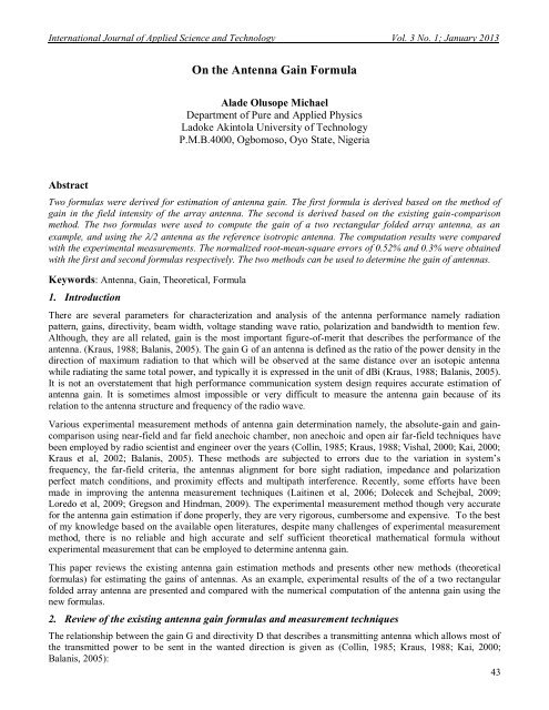
<strong>International</strong> <strong>Journal</strong> <strong>of</strong> <strong>Applied</strong> Science and Technology Vol. 3 No. 1; January 2013<br />
<strong>On</strong> <strong>the</strong> <strong>Antenna</strong> <strong>Gain</strong> <strong>Formula</strong><br />
Alade Olusope Michael<br />
Department <strong>of</strong> Pure and <strong>Applied</strong> Physics<br />
Ladoke Akintola University <strong>of</strong> Technology<br />
P.M.B.4000, Ogbomoso, Oyo State, Nigeria<br />
Abstract<br />
Two formulas were derived for estimation <strong>of</strong> antenna gain. The first formula is derived based on <strong>the</strong> method <strong>of</strong><br />
gain in <strong>the</strong> field intensity <strong>of</strong> <strong>the</strong> array antenna. The second is derived based on <strong>the</strong> existing gain-comparison<br />
method. The two formulas were used to compute <strong>the</strong> gain <strong>of</strong> a two rectangular folded array antenna, as an<br />
example, and using <strong>the</strong> /2 antenna as <strong>the</strong> reference isotropic antenna. The computation results were compared<br />
with <strong>the</strong> experimental measurements. The normalized root-mean-square errors <strong>of</strong> 0.52% and 0.3% were obtained<br />
with <strong>the</strong> first and second formulas respectively. The two methods can be used to determine <strong>the</strong> gain <strong>of</strong> antennas.<br />
Keywords: <strong>Antenna</strong>, <strong>Gain</strong>, Theoretical, <strong>Formula</strong><br />
1. Introduction<br />
There are several parameters for characterization and analysis <strong>of</strong> <strong>the</strong> antenna performance namely radiation<br />
pattern, gains, directivity, beam width, voltage standing wave ratio, polarization and bandwidth to mention few.<br />
Although, <strong>the</strong>y are all related, gain is <strong>the</strong> most important figure-<strong>of</strong>-merit that describes <strong>the</strong> performance <strong>of</strong> <strong>the</strong><br />
antenna. (Kraus, 1988; Balanis, 2005). The gain G <strong>of</strong> an antenna is defined as <strong>the</strong> ratio <strong>of</strong> <strong>the</strong> power density in <strong>the</strong><br />
direction <strong>of</strong> maximum radiation to that which will be observed at <strong>the</strong> same distance over an isotopic antenna<br />
while radiating <strong>the</strong> same total power, and typically it is expressed in <strong>the</strong> unit <strong>of</strong> dBi (Kraus, 1988; Balanis, 2005).<br />
It is not an overstatement that high performance communication system design requires accurate estimation <strong>of</strong><br />
antenna gain. It is sometimes almost impossible or very difficult to measure <strong>the</strong> antenna gain because <strong>of</strong> its<br />
relation to <strong>the</strong> antenna structure and frequency <strong>of</strong> <strong>the</strong> radio wave.<br />
Various experimental measurement methods <strong>of</strong> antenna gain determination namely, <strong>the</strong> absolute-gain and gaincomparison<br />
using near-field and far field anechoic chamber, non anechoic and open air far-field techniques have<br />
been employed by radio scientist and engineer over <strong>the</strong> years (Collin, 1985; Kraus, 1988; Vishal, 2000; Kai, 2000;<br />
Kraus et al, 2002; Balanis, 2005). These methods are subjected to errors due to <strong>the</strong> variation in system’s<br />
frequency, <strong>the</strong> far-field criteria, <strong>the</strong> antennas alignment for bore sight radiation, impedance and polarization<br />
perfect match conditions, and proximity effects and multipath interference. Recently, some efforts have been<br />
made in improving <strong>the</strong> antenna measurement techniques (Laitinen et al, 2006; Dolecek and Schejbal, 2009;<br />
Loredo et al, 2009; Gregson and Hindman, 2009). The experimental measurement method though very accurate<br />
for <strong>the</strong> antenna gain estimation if done properly, <strong>the</strong>y are very rigorous, cumbersome and expensive. To <strong>the</strong> best<br />
<strong>of</strong> my knowledge based on <strong>the</strong> available open literatures, despite many challenges <strong>of</strong> experimental measurement<br />
method, <strong>the</strong>re is no reliable and high accurate and self sufficient <strong>the</strong>oretical ma<strong>the</strong>matical formula without<br />
experimental measurement that can be employed to determine antenna gain.<br />
This paper reviews <strong>the</strong> existing antenna gain estimation methods and presents o<strong>the</strong>r new methods (<strong>the</strong>oretical<br />
formulas) for estimating <strong>the</strong> gains <strong>of</strong> antennas. As an example, experimental results <strong>of</strong> <strong>the</strong> <strong>of</strong> a two rectangular<br />
folded array antenna are presented and compared with <strong>the</strong> numerical computation <strong>of</strong> <strong>the</strong> antenna gain using <strong>the</strong><br />
new formulas.<br />
2. Review <strong>of</strong> <strong>the</strong> existing antenna gain formulas and measurement techniques<br />
The relationship between <strong>the</strong> gain G and directivity D that describes a transmitting antenna which allows most <strong>of</strong><br />
<strong>the</strong> transmitted power to be sent in <strong>the</strong> wanted direction is given as (Collin, 1985; Kraus, 1988; Kai, 2000;<br />
Balanis, 2005):<br />
43
© Centre for Promoting Ideas, USA www.ijastnet .com<br />
G kD,<br />
(1)<br />
Where, k is <strong>the</strong> aperture efficiency <strong>of</strong> <strong>the</strong> antenna to radiate <strong>the</strong> energy presented to its terminals, and it is given<br />
by <strong>the</strong> expression:<br />
max imum effective area <strong>of</strong> <strong>the</strong>antenna (A<br />
em<br />
)<br />
k <br />
, (2)<br />
physical area <strong>of</strong> <strong>the</strong>antenna (A )<br />
( A A , 0 k 1)<br />
em<br />
p<br />
Radiation resistance (R<br />
rad<br />
)<br />
Also, k , (3)<br />
Radiation resistance ohmic loss (R )<br />
( R<br />
L<br />
R<br />
rad<br />
)<br />
While, <strong>the</strong> directivity, D(, ) <strong>of</strong> <strong>the</strong> antenna is <strong>the</strong> ratio <strong>of</strong> <strong>the</strong> Poynting power density S(, ) to <strong>the</strong> power<br />
max imum S( ,<br />
)<br />
density radiated by an isotropic source written as (Kai, 2000): D( ,<br />
)<br />
<br />
,<br />
(4)<br />
2<br />
Pt<br />
/ 4r<br />
Where,<br />
1 1 2<br />
S(<br />
, )<br />
Re( E H)<br />
E , (5)<br />
2<br />
2<br />
2<br />
2A<br />
p<br />
The gains <strong>of</strong> <strong>the</strong> transmitting and receiving antennas separated by a distance r can be related by <strong>the</strong> Friis<br />
<br />
transmission formula which is given as:<br />
PtG<br />
A<br />
Pr<br />
t er<br />
,<br />
(6)<br />
2<br />
4r<br />
Where, A er is <strong>the</strong> effective area <strong>of</strong> <strong>the</strong> receiving antenna which is given as:<br />
2<br />
G<br />
A<br />
r<br />
er<br />
,<br />
(7)<br />
4<br />
Therefore, Equation (6) can be written as:<br />
Pr<br />
<br />
GtGr<br />
,<br />
pt<br />
4r<br />
<br />
Where, is <strong>the</strong> operating wavelength in meters.<br />
2<br />
<strong>On</strong>e <strong>of</strong> <strong>the</strong> antenna gain estimation techniques is called absolute-gain, and it is based on Friis transmission<br />
formula. Under this technique, <strong>the</strong>re are four ways namely; two-antenna method (2AM), Three-antenna Method<br />
(3AM) and o<strong>the</strong>r two: extrapolation method (EM) and Grand Reflection Range Method (GRRM) which depend<br />
on <strong>the</strong> 2AM and 3AM (Vishal, 2000; Balanis, 2005). 2AM is employed for two identical antennas, (transmitting<br />
and receiving antennas), where Friis transmission formula is written in a logarithmic decibel form as:<br />
G<br />
t<br />
G<br />
r<br />
<br />
4r<br />
Pr<br />
log 10log ,<br />
10 <br />
<br />
<br />
Pt<br />
<br />
20<br />
10<br />
Where, G t = gain <strong>of</strong> <strong>the</strong> transmitting antenna in dB, G r = gain <strong>of</strong> <strong>the</strong> receiving antenna dB,<br />
P r = received power in Watt, P t = Transmitted power in Watt, r = distance between transmitting and receiving<br />
antennas in meters.<br />
Since transmitting and receiving antennas are identical, Equation 8 becomes:<br />
1 4r<br />
P <br />
r<br />
<br />
G 20 log<br />
10 10 log<br />
10 , (10)<br />
2<br />
<br />
<br />
t<br />
Gr<br />
<br />
Pt<br />
<br />
<br />
Any <strong>of</strong> <strong>the</strong> parameter: r, , P r and P t can be measured by near-field and far field anechoic chamber, non anechoic<br />
and open air far-field techniques, and <strong>the</strong> gain is computed.<br />
44<br />
L<br />
p<br />
(8)<br />
(9)
<strong>International</strong> <strong>Journal</strong> <strong>of</strong> <strong>Applied</strong> Science and Technology Vol. 3 No. 1; January 2013<br />
The 3AM is employed when <strong>the</strong> transmitting and receiving antennas are not identical. Transmitted and received<br />
powers at <strong>the</strong> antenna terminals are measured between three arbitrary antennas (a, b, c) at a known fixed distance.<br />
The (Friis transmission formula) written in dB, is used to develop three equations and three unknowns as (Vishal,<br />
2000; Balanis, 2005):<br />
4r<br />
Prb<br />
(a - b combination): 20log<br />
10 log<br />
10<br />
, (11)<br />
10 <br />
G <br />
<br />
a<br />
Gb<br />
Pta<br />
<br />
4r<br />
Prc<br />
(a - c combination): 20log<br />
10 log<br />
10<br />
, (12)<br />
10 <br />
G <br />
<br />
a<br />
Gc<br />
Pta<br />
<br />
4r<br />
Prc<br />
(b - c combination): 20log<br />
10 log<br />
10<br />
, (13)<br />
10 <br />
G <br />
<br />
b<br />
Gc<br />
Ptb<br />
<br />
The three equations (11, 12, and 13) are solved to determine <strong>the</strong> unknown gains G a , G b , G c provided r, , P rb , P rc ,<br />
P ta , P tb are known.<br />
The second technique <strong>of</strong> antenna gain estimation is called gain-comparison or gain transfer techniques (GCT or<br />
GTT). The antenna gain is measured by comparing <strong>the</strong> antenna under test, AUT against a known standard<br />
antenna, S gain (Kraus, 1988; Vishal, 2000; Balanis, 2005; Dolecek and Shejbal, 2009). At lower frequencies (<<br />
1GHz) half-wave dipole antenna is employed as <strong>the</strong> standard and at higher frequencies (>1GHz), a high gain<br />
directional horn antenna is employed as <strong>the</strong> standard. The procedure requires two sets <strong>of</strong> measurements. In <strong>the</strong><br />
first, <strong>the</strong> test antenna is used as <strong>the</strong> receiving antenna and <strong>the</strong> received power P r(AUT) is measured and recorded. In<br />
<strong>the</strong> second set, <strong>the</strong> test antenna is replaced by <strong>the</strong> standard gain antenna and <strong>the</strong> received power P r(S) is measured<br />
and recorded.<br />
The gain G AUT <strong>of</strong> <strong>the</strong> antenna under test is <strong>the</strong>n deduced from <strong>the</strong> expression given by (Balanis, 2005):<br />
Pr<br />
( AUT )<br />
10log<br />
10<br />
, (14)<br />
<br />
G<br />
<br />
AUT<br />
GS<br />
<br />
Pr<br />
( S ) <br />
O<strong>the</strong>r efforts made in area <strong>of</strong> <strong>the</strong> antenna measurements are listed as follows:<br />
Laitinen et al, 2006 examined iterative probe-correction technique as a possible method to correct errors<br />
associated with probes from <strong>the</strong> manufacturer. It is because <strong>the</strong>se errors usually lead to inaccurate antenna<br />
measurements.<br />
Dolecek and Schejbal, 2009 verified a simple existing formula for estimation <strong>of</strong> gain <strong>of</strong> <strong>the</strong> shaped-beam antenna.<br />
The results <strong>of</strong> <strong>the</strong> experimental measured gain for five Hogg-horn antennas as examples were comparable with <strong>the</strong><br />
formula:<br />
d b<br />
G k ,<br />
(15)<br />
1<br />
2<br />
Where 1 and 2 are <strong>the</strong> half-power beamwidths in <strong>the</strong> principal planes, and d b is a constant (<strong>the</strong> directivitybeamwidth<br />
product, <strong>the</strong> values <strong>of</strong> 26,000 up to 52,525 are possible).<br />
Loredo et al, 2009 presented a technique to eliminate <strong>the</strong> undesired contributions causing errors in <strong>the</strong> antenna<br />
measurement. In <strong>the</strong> paper titled measurement <strong>of</strong> low gain antenna in non anechoic test sites through wide band<br />
channel characterization and echo cancellation. The measurement techniques based on <strong>the</strong> Fourier Transform<br />
algorithm starts from measurement <strong>of</strong> <strong>the</strong> antenna responses in <strong>the</strong> frequency domain, followed by Fourier<br />
Transformation <strong>of</strong> data to <strong>the</strong> time domain, detection and gating <strong>of</strong> <strong>the</strong> undesired echo in <strong>the</strong> time domain, back to<br />
<strong>the</strong> frequency domain, and retrieval <strong>of</strong> <strong>the</strong> antenna radiation patterns (Characteristics) at <strong>the</strong> frequency <strong>of</strong> interest<br />
(4 GHz – 12 GHz). Seven different standard pyramidal-horn antennas and a monopole antenna were used AUTs<br />
and identical Pyramidal-horn antennas were used as probes. Although <strong>the</strong> technique evaluated under different<br />
conditions demonstrated fairly high accuracy, and even can be adopted for antenna measurement in an anechoic<br />
chamber, it is very costly experimentally and computationally.<br />
45
© Centre for Promoting Ideas, USA www.ijastnet .com<br />
3. Derivation <strong>of</strong> <strong>the</strong> new formulas<br />
Method 1: Array antenna gain<br />
Consider a standard array <strong>of</strong> two rectangular folded antenna side by side as shown in <strong>the</strong> figure 1. Each element <strong>of</strong><br />
circumference C is carrying current I. The far-field electric and magnetic strength <strong>of</strong> one element <strong>of</strong> <strong>the</strong> array in<br />
<strong>the</strong> horizontal plane are respectively given by (Kraus, 1988; Kraus et al, 2002; Balanis, 2005):<br />
60C<br />
<br />
I<br />
-1<br />
E(<br />
)<br />
J1(<br />
C<br />
sin ) , Vm (16)<br />
2r<br />
C<br />
I<br />
-1<br />
H(<br />
)<br />
J1(<br />
C<br />
sin ) , Am (17)<br />
2r<br />
Where,<br />
Circumference <strong>of</strong> <strong>the</strong>loop antenna, C<br />
C<br />
<br />
,<br />
Wavelength, <strong>of</strong> <strong>the</strong> radio wave radiated<br />
is <strong>the</strong> azimuth angle in <strong>the</strong> horizontal plane about <strong>the</strong> vertical plane, and J 1 is <strong>the</strong> first-order Bessel function<br />
given as:<br />
2<br />
4<br />
C sin C sin C sin <br />
1<br />
1!2!<br />
<br />
<br />
<br />
J<br />
1(<br />
C<br />
sin )<br />
1<br />
.......... , (19)<br />
2 <br />
2 2 <br />
Here, <strong>the</strong> Bessel function is approximated to 3 rd term because <strong>the</strong> dimensions (length and breadth) <strong>of</strong> <strong>the</strong><br />
rectangular loop in this work is less than <strong>the</strong> wavelength o <strong>the</strong> radio frequency signal (100 – 650MHz) considered.<br />
As <strong>the</strong> power exponents increase <strong>the</strong> corresponding finite term become insignificant.<br />
Let us concentrate on <strong>the</strong> electric field only. The field intensity E 1 due to <strong>the</strong> single element 1 <strong>of</strong> <strong>the</strong> array can be<br />
expressed as:<br />
E1 E( )<br />
E1<br />
E(<br />
) , (20)<br />
Where, is a dimensionless constant <strong>of</strong> proportionality.<br />
Based on <strong>the</strong> principle <strong>of</strong> pattern multiplication, <strong>the</strong> total field intensity E T due to <strong>the</strong> 2 elements in <strong>the</strong> array can<br />
be expressed as:<br />
1<br />
2!3!<br />
(18)<br />
E T<br />
ET<br />
E1<br />
E2<br />
2E1<br />
, (21)<br />
3<br />
5<br />
60C<br />
sin 1 sin 1 sin <br />
<br />
I C<br />
C<br />
C<br />
<br />
E T<br />
( )<br />
, (22)<br />
r <br />
2 1!2! 2 2!3! 2 <br />
60C<br />
I C<br />
sin 1 3 3sin sin 3<br />
1 5 sin 5<br />
5sin 3<br />
10sin<br />
<br />
( )<br />
C<br />
<br />
C<br />
<br />
,<br />
r 2 16 4 384<br />
16<br />
<br />
<br />
<br />
<br />
<br />
2 4<br />
6<br />
4 6<br />
6<br />
60I<br />
<br />
C 3 10 5 <br />
<br />
<br />
C<br />
C<br />
C<br />
C<br />
C<br />
E T<br />
( )<br />
<br />
sin<br />
<br />
<br />
sin 3 sin 5 ,<br />
<br />
2 64 5824<br />
<br />
<br />
64 5824<br />
<br />
r <br />
5824 <br />
2 4<br />
6<br />
C 3 10 0.5832 0.063773 0.002725<br />
<br />
C<br />
C<br />
a<br />
<br />
2<br />
4<br />
6 <br />
<br />
2 64 5824 <br />
4 6<br />
C 5 0.021258 0.001362<br />
<br />
<br />
C<br />
Let b<br />
<br />
, (25)<br />
4<br />
6<br />
<br />
64 5824 <br />
<br />
6<br />
C 0.000272<br />
<br />
<br />
c<br />
<br />
6<br />
<br />
5824 <br />
<br />
(24)<br />
(23)<br />
46
<strong>International</strong> <strong>Journal</strong> <strong>of</strong> <strong>Applied</strong> Science and Technology Vol. 3 No. 1; January 2013<br />
Therefore,<br />
60I<br />
E T<br />
( )<br />
( asin<br />
bsin 3<br />
csin 5<br />
) ,<br />
r<br />
Assuming <strong>the</strong> total power into <strong>the</strong> array is P, and no heat losses (i.e. A e = A p ):<br />
Power in <strong>the</strong> element 1 is:<br />
2<br />
P ( ) ,<br />
1<br />
I1<br />
R11<br />
R12 (27)<br />
Power in <strong>the</strong> element 2 is:<br />
2<br />
P ( ) ,<br />
2<br />
I<br />
2<br />
R22<br />
R21 (28)<br />
But, R 11 = R 22 ; R 12 = R 21 ; and I 1 = I 2 = I rms .<br />
Where, R 11 and R 22 are <strong>the</strong> self (input) resistances <strong>of</strong> <strong>the</strong> elements 1 and 2 respectively; R 12 and R 21 are <strong>the</strong> mutual<br />
resistances due to <strong>the</strong> elements 2 and 1 respectively.<br />
Therefore, <strong>the</strong> total power to <strong>the</strong> array is;<br />
P P P<br />
Equation 29 yields:<br />
2<br />
2I1<br />
( R11<br />
<br />
12) ,<br />
1 2<br />
R<br />
P<br />
I <br />
,<br />
2(<br />
R 11<br />
R12)<br />
Substituting Equation (30) into (26) yields;<br />
E T<br />
60<br />
( )<br />
<br />
r<br />
2( R<br />
11<br />
P<br />
R<br />
12<br />
(30)<br />
(29)<br />
( asin<br />
bsin 3<br />
csin 5<br />
) ,<br />
)<br />
Using /2 (half-wave dipole) antenna as <strong>the</strong> reference isotropic antenna, assuming no heat losses, <strong>the</strong> current I o at<br />
its terminals under <strong>the</strong> same power supply P is:<br />
I <br />
o<br />
Where, R oo is <strong>the</strong> self-resistance <strong>of</strong> <strong>the</strong> isotropic reference antenna.<br />
The electric far-field intensity due to this isotropic reference antenna is given as (Kraus, 1988):<br />
<br />
cos<br />
cos <br />
RooI<br />
o 2<br />
E<br />
/ 2<br />
( )<br />
<br />
<br />
, (33)<br />
r sin <br />
Substituting Equation (32) into (33) yields:<br />
<br />
cos<br />
cos <br />
Roo<br />
P 2<br />
E<br />
/ 2<br />
( )<br />
<br />
<br />
, (34)<br />
r R sin <br />
oo<br />
P<br />
R<br />
oo<br />
,<br />
The gain in field intensity, GFI, <strong>of</strong> <strong>the</strong> two rectangular folded array antenna in this study according to Kraus 1988<br />
is given as:<br />
ET<br />
( )<br />
GFI ,<br />
E / 2<br />
( )<br />
(35)<br />
Therefore,<br />
GFI 60<br />
a a<br />
<br />
cos 2<br />
bsin<br />
sin 3<br />
c sin sin 5<br />
<br />
1 2 2<br />
<br />
,<br />
2Roo(<br />
R11<br />
R12)<br />
<br />
cos<br />
cos <br />
2 <br />
(35)<br />
(32)<br />
(26)<br />
(31)<br />
47
© Centre for Promoting Ideas, USA www.ijastnet .com<br />
Where,<br />
R<br />
12<br />
<br />
30 2cosh( d)<br />
cosh[ (<br />
2<br />
,<br />
<br />
Method 2: General antenna gain<br />
d<br />
2<br />
L<br />
2<br />
L)]<br />
cosh[ (<br />
d<br />
2<br />
L<br />
2<br />
<br />
L)]<br />
,<br />
Applying <strong>the</strong> Friis transmission formula (Equation 6) to <strong>the</strong> gain-comparison formula (Equation 14) yields gain<br />
formula which can be used for all antennas and is given as:<br />
A<br />
( )<br />
10log<br />
10<br />
, (37)<br />
<br />
er AUT<br />
G<br />
<br />
AUT<br />
GS<br />
<br />
Aer(<br />
S ) <br />
4. Results and Discussion<br />
In this paper two formulas were derived for estimation <strong>of</strong> antenna gain. <strong>On</strong>e <strong>of</strong> <strong>the</strong> formulas is derived based on<br />
<strong>the</strong> method <strong>of</strong> gain in <strong>the</strong> field intensity <strong>of</strong> <strong>the</strong> array antenna earlier published by Kraus, 1988, and <strong>the</strong> formula is<br />
meant for array antenna gain. The second formula can be used to determine <strong>the</strong> gain <strong>of</strong> all antennas. It is derived<br />
based on <strong>the</strong> existing gain-comparison method. The two formulas were used to compute <strong>the</strong> gain <strong>of</strong> a two<br />
rectangular folded array antenna, as an example, using <strong>the</strong> /2 antenna as <strong>the</strong> reference isotropic antenna. The<br />
results <strong>of</strong> <strong>the</strong> computation were compared with <strong>the</strong> experimental measurement results <strong>of</strong> <strong>the</strong> antenna gain. It is<br />
observed that <strong>the</strong> normalized root-mean-square errors <strong>of</strong> 0.52% and 0.3% were obtained when <strong>the</strong> method 1 and<br />
method 2 were respectively compared with <strong>the</strong> measured gain <strong>of</strong> <strong>the</strong> antenna. The two methods can be used to<br />
determine <strong>the</strong> gain <strong>of</strong> antennas.<br />
5. Conclusion<br />
It is evident from this study that <strong>the</strong> two formulas derived for antenna gain calculation can be adopted by <strong>the</strong><br />
antenna designer as gain prediction formulas for <strong>the</strong> array antennas and general antennas as <strong>the</strong> case may be.<br />
(36)<br />
Figure 1: Experimental set up showing standard two rectangular folded<br />
array antenna employed in <strong>the</strong> measurements, and connected to <strong>the</strong> GSP<br />
810 spectrum analyzer as <strong>the</strong> receiver.<br />
48
<strong>Gain</strong> in dBi<br />
<strong>International</strong> <strong>Journal</strong> <strong>of</strong> <strong>Applied</strong> Science and Technology Vol. 3 No. 1; January 2013<br />
25<br />
20<br />
Method1<br />
Method2<br />
Experimental Measurements<br />
15<br />
10<br />
5<br />
0<br />
0 100 200 300 400 500 600<br />
Frequency in MHz<br />
Figure 2: Showing <strong>the</strong> plot <strong>of</strong> gain versus frequency to compare <strong>the</strong> two<br />
formulas (methods 1 and 2) with <strong>the</strong> experiment.<br />
References<br />
Dolecek. R and Schejbal. V (Feb 2009): Estimation <strong>of</strong> <strong>Antenna</strong> <strong>Gain</strong>. IEEE <strong>Antenna</strong>s and Propagation magazine,<br />
ISSN: 1045-9243, Vol.51, No.1, pp. 124-125.<br />
Loredo.S , Leon.G , Zapatero.S and Las-Heras.F (Feb 2009):Measurement <strong>of</strong> Low-<strong>Gain</strong> <strong>Antenna</strong>s in Non-<br />
Anechoic Test Sites through Widebaand Channel Characterization and Echo Cancellation. IEEE<br />
<strong>Antenna</strong>s and Propagation Magazine, ISSN: 1045-9243, Vol.51, No.1, pp. 128-135.<br />
Collin R.E (1985): <strong>Antenna</strong>s and Radiowave Propagation, Mc Graw-Hill, New York<br />
J. D. Kraus, ‘‘<strong>Antenna</strong>s’’, 2 nd Edition, ISBN: 0-07-035422-7, McGraw-Hill Inc., USA, 1988.<br />
J. D. Kraus, R. J. Marhefka, B. A. Muuk, A. Lehto, P. Vainikainen, E. H. Newman, and C.<br />
Walker, ‘‘<strong>Antenna</strong>s for All Applications’’, Third Edition, ISBN: 0-07-232103-2, McGraw-Hill, USA, 2002.<br />
C. A. Balanis, ‘‘<strong>Antenna</strong> Theory’’ 3 rd Edition, ISBN 0-471-66782-X, John Wiley & Sons Ltd., USA, 2005.<br />
Laitinen. T, Pivnenko. S and Breinbjerg. O (Aug2006):Application <strong>of</strong> <strong>the</strong> Iterative Probe-Correction Technique<br />
for a High-Order Probe in Spherical Near-Field <strong>Antenna</strong> Measurements. IEEE <strong>Antenna</strong>s and Propagation<br />
Magazine, Vol.48, No.4, pp. 179-185.<br />
Vishal.B, Nicholas.B, Huy.N and Alexander.B(2000): <strong>Antenna</strong> <strong>Gain</strong> Measurement-EE117 Laboratory Manual,<br />
UC-Riverside, USA.<br />
Kia. C, ‘‘RF and Microwave Wireless Systems’’, ISBN: 0-47135199-7, John Willey and Sons Inc., New York,<br />
2000.<br />
Gregson. S. F and Hindman. G. E (2009): Conical Near-Field <strong>Antenna</strong> Measurements. IEEE <strong>Antenna</strong> and<br />
Propagation Magazine, ISSN: 1045-9243, Vol. 51, No. 1, pp. 193 – 201.<br />
49