A Time-Dependent Enhanced Support Vector Machine For Time ...
A Time-Dependent Enhanced Support Vector Machine For Time ...
A Time-Dependent Enhanced Support Vector Machine For Time ...

You also want an ePaper? Increase the reach of your titles
YUMPU automatically turns print PDFs into web optimized ePapers that Google loves.
Table 2: <strong>Support</strong> <strong>Vector</strong> Regression and <strong>Time</strong>-<strong>Dependent</strong> <strong>Support</strong> <strong>Vector</strong> Regression empirical loss and its<br />
derivative<br />
<strong>Support</strong> <strong>Vector</strong> Regression <strong>Time</strong>-<strong>Dependent</strong> <strong>Support</strong> <strong>Vector</strong> Regression<br />
Empirical loss l 1(x i,y i,w) max(0, |w T x i – y i| – ǫ) max(0, |w T x i – y i| – ǫ)<br />
Derivative l 1(x ′ i,y i,w) sign(w T x i–y i) if |w T x i–y i| > ǫ; sign(w T x i – y i) if |w T x i – y i| > ǫ;<br />
otherwise 0 otherwise 0<br />
<strong>Time</strong>-<strong>Dependent</strong> loss 0 for all samples max (0, |(w T x i – y i) – (w T x i−1 – y i−1)| - ǫ t )<br />
l 2(x i,y i,w,x i−1,y i−1) for distribution shift samples; otherwise 0<br />
Derivative 0 for all samples sign((w T x i–y i)–(w T x i−1–y i−1))<br />
l 2(x ′ i,y i,w,x i−1,y i−1)<br />
if |(w T x i–y i)–(w T x i−1 – y i−1)| > ǫ t<br />
for distribution shift samples, otherwise 0<br />
l 2(x i,y i,w, x i−1,y i−1) is<br />
{ | (w T x i −y i )−(w T x i−1 −y i−1 ) | x i−1 is dist. shift<br />
0 otherwise<br />
(5)<br />
where it can be seen that if x i−1 is not a distribution shift<br />
sample, then no loss is incurred. Otherwise, the loss is equal<br />
to the amount of difference between the prediction error for<br />
x i and theprediction error for x i−1. Wecan further incorporate<br />
a tolerable error term ǫ t to yield a soft time-dependent<br />
loss. This is shown in Table 2. By linearly combining our<br />
time-dependentloss function with the standardloss function<br />
for SVM regression, we formulate a new type of SVM, which<br />
we henceforth refer to as TiSe SVM (time sensitive SVM).<br />
Observe that if no samples are classified as distribution shift<br />
samples, then a TiSE SVM is exactly the same as SVM. Using<br />
the definitions from Table 2, the modified empirical loss<br />
and regularized risk function for TiSE SVM have the form<br />
R TiSe<br />
emp (w) = 1 n<br />
n∑<br />
(l 1 (x i ,y i ,w)+λ∗l 2 (x i ,y i ,w,x i−1 ,y i−1 ))<br />
i=1<br />
(6)<br />
L(w ∗ ) = argmin w φw T w+R TiSe<br />
emp (w) (7)<br />
The λ parameter is a regularization parameter that determines<br />
the extent to which we want to minimize the timedependent<br />
loss function. Larger values of λ will result in the<br />
time-dependent loss function having more influence in the<br />
overall error. We investigate the effect of this parameter in<br />
the experimental section, in order to determine values suitable<br />
for our experimental work.<br />
3.4 SVM Regression time-dependent loss optimization<br />
The new SVM regression which incorporates the timedependent<br />
loss will now have the following form:<br />
L TiSe (w ∗ ) = 1 ∑ n<br />
∑ n<br />
2 ||w||2 +C 1 (ξ + i +ξ − i )+C 2 (ζ + i +ζ − i )<br />
i=1<br />
i=2<br />
subject to<br />
⎧<br />
〈w,x i〉+b+ǫ+ξ + i ≥ y i<br />
〈w,x ⎪⎨ i〉+b−ǫ−ξ − i<br />
≤ y i<br />
(〈w,x i〉−y i)−(〈w,x i−1〉−y i−1)+ǫ t +ζ + i<br />
≥ 0<br />
(〈w,x i〉−y i)−(〈w,x i−1〉−y i−1)−ǫ t −ζ − i<br />
≤ 0<br />
⎪⎩<br />
ξ + i ,ξ− i ,ζ+ i ,ζ− i<br />
≥ 0<br />
(8)<br />
(9)<br />
where ǫ t is the allowed value of the differences in the time<br />
sensitiveerror, andζ + andζ − areslackvariablesforthetime<br />
sensitive loss. In order to solve this, we introduce Lagrange<br />
multipliers α + i<br />
≥ 0, α − i<br />
≥ 0, µ + i<br />
≥ 0 and µ − i<br />
≥ 0 for all i,<br />
β + i , β− i , η+ i<br />
and η − i<br />
for i = 2...n:<br />
∑ n n∑<br />
L P =C 1 (ξ + i +ξ − i )+C 2 (ζ + i +ζ − i )+ 1 2 ||w||2<br />
i=1 i=2<br />
n∑<br />
n<br />
− (µ + i ξ+ i +µ − i ξ− i )− ∑<br />
α + i (ǫ+ξ+ i −y i +〈w,x i 〉+b)<br />
i=1<br />
i=1<br />
n∑<br />
− α − i (ǫ+ξ− i +y i −〈w,x i 〉−b)<br />
i=1<br />
n∑<br />
−λ (η + i ζ+ i +η − i ζ− i )<br />
i=2<br />
n∑<br />
−λ β + i ((〈w,x i〉−y i )−(〈w,x i−1 〉−y i−1 )+ǫ t +ζ + )<br />
i=2<br />
n∑<br />
−λ β − i (−(〈w,x i〉−y i )+(〈w,x i−1 〉−y i−1 )+ǫ t +ζ − )<br />
i=2<br />
(10)<br />
Differentiating with respect to w, b, ξ + i , ξ− i , ζ+ i<br />
and ζ − i<br />
and<br />
setting the derivatives to 0, we will get the dual form:<br />
n∑<br />
n∑<br />
L D = (α + i −α − i )y i +λ (β + i −β − i )y i<br />
i=1<br />
i=2<br />
n∑<br />
n∑<br />
−λ (β + i −β − i )y i−1 −ǫ (α + i +α − ∑ n<br />
i )−λǫt (β + i +β − i )<br />
i=2<br />
i=1<br />
− 1 n∑<br />
(α + i −α − i<br />
2<br />
)(α+ j −α− j )x ix j<br />
i,j=1<br />
i=2<br />
− 1 ∑ n<br />
2 λ2 (β + i −β − i )(β+ j −β− j )(x ix j −2x i x j−1 +x i−1 x j−1 )<br />
−λ<br />
i,j=2<br />
n∑<br />
(α + i −α − i )(β+ j −β− j )(x ix j −x i x j−1 )<br />
i=1,j=2<br />
(11)<br />
This form allows for a Quadratic Programming to be applied<br />
in order to find w and b. Also, it can be noticed that if<br />
we need to move to a higher dimensionality space x → ψ(x),<br />
such that a kernel function exists k(x ix j) = ψ(x i)ψ(x j), we<br />
can do so as L D can be kernelized.