Is B . n dS = 0,

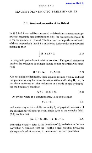
CHAPTER 2 

MAGNETOKINEMATIC PRELIMINARIES 

2.1. Structural properties of the B-field 

In §§ 2.1-2.4 we shall be concerned with basic instantaneous properties 

of magnetic field distributions B(x); the time dependence of B 

is for the moment irrelevant. The first, and perhaps the most basic, 

of these properties is that if S is any closed surface with unit outward 

normal n, then 

Is B . n dS = 0, 

i.e. magnetic poles do not exist in isolation. This global statement 

implies the existence of a single-valued vector potential A(x) satisfying 

B=VAA, V.A=O. (2.2) 

A is not uniquely defined by these equations since we may add to it 

the gradient of any harmonic function without affecting B; but, in 

problems involving an infinite domain, A is made unique by imposing 

the boundary condition 

A+O as(x(-+m. (2.3) 

At points where B is differentiable, (2.1) implies that 

V.B=O, (2.4) 

and across any surface of discontinuity S, of physical properties of 

the medium (or of other relevant fields such as the velocity field), 

(2.1) implies that 

[n . B] = (n . B)+ - (n . B)- = 0, (2.5) 

where the + and - refer to the two sides of S,, and n is now the unit 

normal on S, directed from the - to the + side. We shall always use 

the square bracket notation to denote such surface quantities.

The lines of force of the B-field (or ‘B-lines’) are determined as 

the integral curves of the differential equations 

A B-line may, exceptionally, close on itself. More generally it may 

cover a closed surface S in the sense that, if followed far enough, it 

passes arbitrarily near every point of S. It is also conceivable that a 

B-line may be space-filling in the sense that, if followed far enough, 

it passes arbitrarily near every point of a three-dimensional region 

V; there are no known examples of solenoidal B-fields, finite and 

differentiable everywhere, with this property, but it is nevertheless a 

possibility that no topological arguments have yet been able to 

eliminate, and indeed it seems quite likely that B-fields of any 

degree of complexity will in general be space-filling. 

Now let C be any (unknotted) closed curve spanned by an open 

orientable surface S with normal n. The flux @ of B across S is 

defined by 

(2.7) 

where the line integral is described in a right-handed sense relative 

to the normal on S. Afiux-tube is the aggregate of B-lines passing 

through a closed curve (usually of small or infinitesimal extent). By 

virtue of (2.1), @ is constant along a flux-tube. 

A measure of the degree of structural complexity of a B-field is 

provided by a set of integrals of the form 

I, = Jvm A. B d3x (m = 1,2,3, - a), 

(2.8) 

where V, is any volume with surface S,,, on which n . B = 0. 

Suppose, for example, that B is identically zero except in two 

flux-tubes occupying volumes V1 and V2 of infinitesimal crosssection 

following the closed curves C1 and C2 (fig. 2.l(a)) and let 

and

MAGNETOKINEMATIC PRELIMINARIES 15 

2 

(4 (6) 

Fig. 2.1 (a) The-two flux-tubes are linked in such a way as to give positive 

magnetic helicity. (b) A flux-tube in the form of a right-handed trefoil knot; 

insertion of equal and opposite flux-tube elements between the points A 

and B as indicated gives two tubes linked as in (a). 

configuration as drawn, evidently B d3x may be replaced by Ql dx 

on C1 and

16 MAGNETIC FIELD GENERATION IN FLUIDS 

More generally, if the Vm can be chosen so that Vco =u2=1 Vm, 

then 

(2.13) 

If a single flux-tube (with flux a) winds round itself before closing 

(i.e. if it is knotted) then the integral I, for the associated magnetic 

field will in general be non-zero. Fig. 2.l(b) shows the simplest 

non-trivial possibility: the curve C is a right-handed trefoil knot; 

insertion of the two self cancelling elements between the points A 

and B indicates that this is equivalent to the configuration of fig. 

2.l(a) with a1 =@2=Q) so that I=2Q2. Knotted tubes may 

always be decomposed in this way into two or more linked tubes. 

It may of course happen that A . B 0; it is well known that this is 

the necessary and sufficient condition for the existence of scalar 

functions q(x) and Q(x) such that 

A=(CIVcp, B=Vt,b~Vcp. (2.14) 

In this situation, the B-lines are the intersections of the surfaces 

cp = cst., Q = cst., and the A-lines are everywhere orthogonal to the 

surfaces cp = cst. It is clear from the above discussion that B-fields 

having linked or knotted B-lines cannot admit such a representation. 

The same limitation applies to the use of Clebsch variables 

9, +, x, defined (if they exist) by the equations 

A=+Vcp+Vx, B=V@AV~. (2.15) 

For example, if B is a field admitting such a representation, with cp, t,b 

and x single-valued differentiable functions of x, then 

and 

A. B = VX . (VQ ~Vcp), 

= lVm 

VX .(Vt,b A Vcp) d3x 

(2.16)


since n . B = 0 on Sm. Conversely, if Im # 0 (as will happen if the 

B-lines are knotted or linked), then (2.15) is not a possible global 

representation for A and B (although it may be useful in a purely 

local analysis). 

The characteristic local structure of a field for which A. B is 

non-zero may be illustrated with reference to the example (in 

Cartesian coordinates) 

B = (Bo, 0, 0), 

A= (Ao,-;B~Z, 

$Boy), (2.17) 

where A. and Bo are constants; note that possible Clebsch variables 

are 

(2.18) 

there is here no closed surface on which n . B = 0, and the problem 

noted above does not arise. Clearly A. B = AoBo, and the A-lines 

are the helices with parametric representation 

x = (2Ao/Bo)t, y = cos t, z = sin t. (2.19) 

These helices are right-handed or left-handed according as AoBo is 

positive or negative. 

The quantity A. (V A A) for any vector field A(x) is called the 

helicity density of the field A; its integral I, over V,, is then the 

helicity of A; the integrals I,,, over V, can be described as ‘partial’ 

helicities. The helicity density is a pseudo-scalar quantity, being the 

scalar product of a polar vector and an axial vector; its sign 

therefore changes under change from a right-handed to a lefthanded 

frame of reference. A field A that is ‘reflexionally symmetric’ 

(i.e. invariant under the change from a right-handed to a 

left-handed reference system represented by the reflexion x’ = -x) 

must therefore have zero helicity density. The converse is 

not true, since of course other pseudo-scalar quantities such as 

(V A A). V A (V A A) may be non-zero even if A. (V A A)= 0. 

2.2. Magnetic field representations 

In a spherical geometry, the most natural coordinates to use are 

spherical polar coordinates (r, 8, q) related to Cartesian coordinates


(x, Y, 2) by 

x = r sin 8 cos p, y = r sin 8 sin p, z = r cos 8. (2.20) 

Let us first recall some basic results concerning the use of this 

coordinate system. 

Let +(r, 8, cp) be any scalar function of position. Then 

where 

L~+ 

The vector identity 

1 a a 1 a2 

a0 sin 8 ap 

= (- -sin e-+T 7). 

sin 8 a0 

(2.21) 

(2.22) 

(x A V )2~ r2V2+ - 2(x . V)+ -x . (x . V)V$ (2.23) 

leads to the identification 

L2$ = (X A v)2$. (2.24) 

L2 is the angular momentum operator of quantum mechanics. Its 

eigenvalues are-n(n + 1) (n = 0, 1,2, . . .), and the corresponding 

eigenfunctions are the surface harmonics 

n 

Sn(8, cp) = 2 A,"P,"(cos 8) e'"', (2.25) 

m =O 

where P:(cos 8) are associated Legendre polynomials and the A," 

are arbitrary complex constants; i.e. 

L2Sn =iln(n + l)Sn. (2.26) 

Now let f(r, 8,p) be any smooth function having zero average 

over spheres r = cst., i.e. 

277 77 

47rr2(f) = I f(r, 8, p) sin 8 d8 dp = 0. (2.27) 

0 0 

We may expand f in surface harmonics 

the term with n = 0 being excluded by virtue of (2.27). The func-


tions Sn satisfy the orthogonality relation 

and so the coefficients fn (r) are given by 

(SnSnr) = 0, (n# n'), (2.29) 

If now 

then clearly the operator L2 may be inverted to give 

the result also satisfying ($) = 0. 

Note that any function of the form f = x. V A A, where A is an 

arbitrary smooth vector field, satisfies the condition (2.27); for 

I,,.) * 

A dS = J,s(r) 6,r) 

n . (V A A) dS = r V . (V A A) dV= 0, 

(2.33) 

where S(r) is the surface of the sphere of radius r and V(r) its 

interior. 

A toroidal magnetic field BT is any field of the form 

BT = V A (xT(x)) = -X AVT, (2.34) 

where T(x) is any scalar function of position. Note that addition of 

an arbitrary function of r to T has no effect on BT, so that without 

loss of generality we may suppose that (T) = 0. Note further that 

x . BT = 0, so that the lines of force of BT ('BT-lines') lie on the 

spherical surfaces r = cst. 

A poloidal magnetic field BP is any field of the form 

BP = VA V A (xP(x)) = -VA (X AVP), (2.35) 

where P(x) is any Scalar function of position which again may be 

assumed to satisfy (P) = 0. BP does in general have a non-zero radial 

component. 

It is clear from these definitions that the curl of a toroidal field is a 

poloidal field. Moreover the converse is also true; for 

V A V A V A (xP) = -V2V A (xP) = -V A (xV'P). (2.36)


The latter identity can be trivially verified in Cartesian coordinates. 

Now suppose that 

Then 

B = B, +B, = V A V A (xP) +V A (xT). 

(2.37) 

x . B = -(x A V)2P, x . (V A B) = -(x A V)2T, (2.38) 

so that P and T may be obtained in the form 

P= -L-2(~. B), 

T= -L-2~. (V A B). (2.39) 

Conversely, given any solenoidal field B, if we define P and T by 

(2.39), then (2.37) is satisfied, i.e. the decomposition of B into 

poloidal and toroidal ingredients is always possible. 

If we ‘uncurl’ (2.37), we obtain the vector potential of B in the 

form 

A = V A (xP) +xT+ VU, (2.40) 

where U is a scalar ‘funetion of integration’. Since V . A = 0, U and 

T are related by 

V2U = -V. (xT) (2.41) 

By virtue of this condition, xT + VU may itself be expressed as a 

poloidal field: 

xT+VU = V A V A (xS), 

The toroidal part of A is simply 

Axisymmetric fields 

S = -L-2(r2T+x. VU). 

(2.42) 

AT = V A (xP) = -X AVP. (2.43) 

A B-field is axisymmetric about a line Oz (the axis of symmetry) if it 

is invariant under rotations about Oz. In this situation, the defining 

scalars P and T of (2.37) are clearly independent of the azimuth 

angle cp, i.e. T = T(r, 0), P = P(r, 0). The*toroidal field BT = -x A VT 

then takes the form 

B~ = (o,o, B~), B~ = -aT/ae, (2.44)


and so the BT-lines are circles r = cst., 8 = cst. about Oz. Similarly, 

AT = (0, 0, A,), A, = -aP/ae, (2.45) 

and, correspondingly, in spherical polars, 

where 

(2.46) 

x = r sin 8, A, = -r sin 8 dP/a8. (2.47) 

The scalar x is the analogue of the Stokes stream function $(r, 8) for 

incompressible axisymmetric velocity fields. The Bp-lines are 

given by x = cst., and the differential 

27r dx = (B, dr -BJ d8)27rr sin 8 (2.48) 

represents the flux across the infinitesimal annulus obtained by 

rotating about Oz the line element joining (r, 0) and (r + dr, 8 +do). 

It is therefore appropriate to describe x as the flux-function of the 

field Bp. 

When the context allows no room for ambiguity, we shall drop the 

suffix cp from B, and A,, and express B in the simple form 

where i, is a unit vector in the cp-direction’. 

The two-dimensional analogue 

B = Bi, +V A (/lip), (2.49) 

Geometrical complications inherent in the spherical geometry frequently 

make it desirable to seek simpler representations. In particular, 

if we are concerned with processes in a spherical annulus 

rl < r < r2 with r2 - rl

1 


Fig. 2.2 Local Cartesian coordinate system in a spherical annulus geometry; 

Ox is directed south, Oy east, and Oz vertically upwards. 

and P and T are given by 

V;P = -4,. B, V;T= -i, . (V A B), (2.51) 

where Vi is the two-dimensional Laplacian 

V; = (i, A v )~ = a2/ax + d2/ay ’. (2.52) 

If the field B is independent of the coordinate y (the analogue of 

axisymmetry), then P = P(x, z), T= T(x, z). The ‘toroidal’ field 

becomes 

and the ‘poloidal’ field becomes 

BT = Bi,, B = -dT/dx, (2.53) 

Bp=V~(Aiy), A = -aP/ax. (2.54) 

The Bp-lines are now given by A(x, z) = cst., and A is the fluxfunction 

of the Bp-field. 

Quite apart from the spherical annulus context, two-dimensional 

fields are of independent interest, and consideration of idealised 

two-dimensional situations can often provide valuable insights. It is 

then in general perhaps more natural to regard Oz as the direction 

of invariance of B and to express B in the form 

B = V A (A(x, y)i,) + B(x, y)i,. (2.55)


2.3. Relations between electric current and magnetic field 

In a steady situation, the magnetic field B(x) is related to the electric 

current distribution J(x) by Ampere’s law; in integral form this is 

fc B.dx=po J.ndS, (2.56) 

where S is any open orientable surface spanning the closed curve C, 

and po is a constant associated with the system of units used2. If B is 

measured in Wb m-’ (1 Wb m-’ = 104 gauss) and J in A m-2, then 

I, 

po = 4~ x 10-7 Wb A-’ m-l. (2.57) 

It follows from (2.56) that in any region where B and J are 

differentiable, 

VAB=~J, V.J=O, (2.58) 

and the corresponding jump conditions across surfaces of discontinuity 

are 

[n AB] = p Js, [n . J] = 0, (2.59) 

where Js (A m-l) represents surface current distribution. Surface 

currents (like concentrated vortex sheets) can survive only if dissipative 

processes do not lead to diffusive spreading, i.e. only in a- 

perfect electrical conductor. In fluids or solids of finite conductivity, 

we may generally assume that Js = 0, and then (2.59) together with 

(2.5) implies that all components of B are continuous: 

[B] = 0. (2.60) 

In an unsteady situation, (2.56) is generally modified by the 

inclusion of Maxwell’s displacement current; it is well known 

however that this effect is negligible in treatment of phenomena 

whose time-scale is long compared with the time for electromagnetic 

waves to cross the region of interest. This condition is certainly 

satisfied in the terrestrial and solar contexts, and we shall therefore 

neglect displacement current throughout; this has the effect of 

filtering electromagnetic waves from the system of governing equa- 1 

/T 

I - ‘/ 

. 

Permeability effects are totally unimportant in the topics to be considered and may 

be ignored from the outset.


tions. The resulting equations are entirely classical (i.e. nonrelativistic) 

and are sometimes described as the 'pre-Maxwell equations'. 

In terms of the vector potential A defined by (2.2), (2.58) 

becomes the (vector) Poisson's equation 

V2A = -poJ. (2.61) 

Across discontinuity surfaces, A is in general -continuous (since 

B=VnA is in general finite) and (2.60) implies further that the 

normal gradient of A must also be continuous; i.e. in general 

[A] = 0, [(n . V)A] = 0. (2.62) 

Multipole expansion of the magnetic field 

Suppose now that S is a closed surface, with interior V and exterior 

e, and suppose that J(x) is a current distribution entirely confined to 

excluding the possibility of surface current on S, 

V, i.e. J = 0 in Q; 

we must then also have n . J = 0 on S. From (2.58), B is irrotational 

in p, and so there exists a scalar potential q(x) such that, in 

B = -VT, V2q = 0. (2.63) 

j , Note that in general !P is not single-valued; it is, however, singlet 

' valued if 9 is simply-connected, and we shall assume this to be the 

i case. We may further suppose that !P+ 0 as 1x1+ W. 

\ 

Relative to an origin 0 in V, the general solution of (2.63) 

' j 1 

vanishing at infinity may be expressed in the form 

CO 

-_ \)q(x) = c !P(~)(x), ~(~'(x) 

/ fl=l 

= -Pg! s(r-l),ij ... s ; (2.64) 

here is the multipole moment tensor of rank n, r = 1x1, and a 

suffix i after the comma indicates differentiation with respect to xi. 

The term with n = 0 is omitted by virtue of (2.1). The terms with 

n = 1,2 are the dipole and quadrupole terms respectively; in vector 

notation 

W)(x) = -p . V(r-'), 

and similarly for higher terms. 

q(2)(x) = +*': VV(P), 

(2.65)


The field B in 

clearly has the expansion 

00 

Wx) = C ~'"'(x), B?'(x) = Pt!s(T-l),ij ... sa, (2.66) 

n=l 

and, since V2(r-') = 0 in the expression for B'"' may be expressed 

in the form B'"' = V A A'"' where 

The first two terms of the expansion for the vector potential, 

corresponding to (2.65), thus have the form 

A(')(x) = -p(') A V(r-'), 

A(2)(x) = ---P'~' i\ VV(r-'). (2.68) 

The tensors p'"' may be determined as linear functionals of J(x) as 

follows. The solution of (2.61) vanishing at infinity is 

A(x) = lv (x - x'1-l J(x') d3x', (2.69) 

(and it may be readily verified using V . J = 0, n . J = 0 on S, that this 

satisfies V . A = 0). The function Ix - x'1-l has the Taylor expansion 

(2.70) 

Substitution in (2.69) leads immediately to A = 1 A'"'(x) where 

Comparison with (2.67) then gives the equivalent relations 

(2.71) 

In particular, for the terms n = 1,2 we have 

(2.73)


Axis y mmetric fields 

If J(x) is axisymmetric about the direction of the unit vector i, = e, 

then these results can be simplified. Choosing spherical polar 

coordinates (r, 8,q) based on the polar axis Oz, we have evidently 

dl) = CL(% p(') = $po 11 Jq(r, 8)r3 sin2 8 dr d8. 

(2.74) 

Likewise, must be axisymmetric about Oz ; and since pj:) = 0 

from (2.733), it must therefore take the form 

(2, = (2) 

prnj E.L (ernej -iarnj). 

(2.75) 

Putting m = 3, j = 3 in (2.73) and (2.75) then gives p(2) in the form 

(2.76) 

In this axisymmetric situation, the expansion (2.64) clearly has the 

form 

(2.77) 

2.4. Force-free fields 

We shall have frequent occasion to refer to magnetic fields for which 

B is everywhere parallel to J = pOIV A B and it will therefore be 

useful at this stage to gather together some properties of such 

fields3, which are described as 'force-free' (Lust & Schluter, 1954) 

since the associated Lorentz force J A B is of course identically zero. 

For any force-free field, there exists a scalar function of position 

K(x) such that 

VAB=KB, B.VK=O, (2.78) 

the latter following from V . B= 0. K is therefore constant on 

B-lines, and if B-lines cover surfaces then K must be constant on 

each such surface. A particularly simple situation is that in which K 

is constant everywhere; in this case, taking the curl of (2.78) 

In general, a vector field B(x), with the property that V A B is everywhere parallel to 

B, is known as a Beltrami field.

'' 

MAGNETO KIN EM AT1 C P R E L I M I N A R I E S 27 

immediately leads to the Helmholtz equation 

(v2 + K~)B = 0. (2.79) 

Note however that this process cannot in general be reversed: a field 

B that satisfies (2.79) does not necessarily satisfy either of the 

equations V A B = f KB. 

The simplest example of a force-free field, with K = cst., is, in 

Cartesian coordinates, 

B = Bo(sin Kz, cos Kz, 0). (2.80) 

The property V A B = KB is trivially verified. The B-lines, as indicated 

in fig. 2.3(a), lie in the x-y plane and their direction rotates 

t 

(4 (b) 

Fig. 2.3 (a) Lines of force of the field (2.80) (with K > 0). 0 indicates a line 

in the positive y-direction (i.e. into the paper), and 0 indicates a line in the 

negative y-direction; the lines of force rotate in a left-handed sense with 

increasing z. Closing the lines of force by means of the dashed segments 

leads to linkages consistent with the positive helicity of the field. (b) Typical 

helical lines of force of the field (2.82); the linkages as illustrated are 

negative, and therefore correspond to a negative value of K in (2.82). 

with increasing z in a sense that is left-handed or right-handed 

according as K is positive or negative. The vector potential of B is 

simply A = K-lB, so that its helicity density is uniform: 

A. B = K-'B2 = K-'B$ (2.8 1)


If we imagine the lines of force closed by the dashed lines as 

indicated in the figure, then the resulting linkages are consistent 

with the discussion of 8 2.1. 

A second example (fig. 2.3(b)) of a force-free field, with K again 

constant, is, in cylindrical polars (s, cp, z), 

where J, is the Bessel function of order n. Here the B-lines are 

helices on the cylinders s = cst. Again A = K-lB, and 

A . B = K1B2 = K-'Bi[(J1(Ks))2 + (Jo(Ks))2], (2.83) 

and again any simple closing of lines of force would lead to linkages 

(which are negative, corresponding to a negative value of K, in Fig. 

2.3(6). 

In both these examples, the J-field extends to infinity. There are 

in fact no force-free fields, other than BE 0, for which J is confined 

(as in 8 2.3) to a finite volume V and B is everywhere differentiable 

and O(f3) at infinity4. To prove this, let Ki be the Maxwell stress 

tensor, given by 

with the properties 

Tj = pO1(B,B, -$B2Sij), (2.84) 

(J AB)~ = Tii, Ti = -(2pO)-lB2, (2.85) 

and suppose that J A B = 0. Then 

0 = xiKij d3x = Ism 

nixiTi dS -\ Ti d3x, (2.86) 

the volume integrals being over all space. Now since B = O(rV3) as 

r + 00, rj = O(r-6) and so the integral over S, vanishes. Hence the 

integral of B2 vanishes, and so B = 0. The proof fails if surfaces of 

discontinuity of B (and so of Kj) are allowed, since then further 

surface integrals which do not in general vanish must be included in 

(2.86). 

This condition means of course that the only source for B is the current distribution 

J, and there are no further 'sources at infinity'. The leading term of the expansion 

(2.66) is clearly O(F~). It is perhaps worth noting that the proof still goes through 

under the weaker condition B=o(~-~'~) corresponding to finiteness of the 

magnetic energy I Ki d3x.


Force -free fields in spherical geometry 

We can however construct solutions of (2.78) which are force-free 

in a finite region V and current-free in the exterior region and 

which do not vanish at infinity. This can be done explicitly (Chandrasekhar, 

1956) as follows, in the important case when V is the 

sphere r < R. First let 

(2.87) 

where KO is constant. We have seen in 8 2.2 that, under the poloidal 

and toroidal decomposition 

we have 

B = V A V A XP + V A xT, (2.88) 

VAB= -VA (XV~P)+VA v A (xT), (2.89) 

and so (2.78) is satisfied provided 

T=KP and (V2+K2)P=0. (2.90) 

Here K is discontinuous across r = R; but continuity of B ((2.60)) 

requires that T, P and dP/dr be continuous across r = R, or equivalently 

P=O, [dP/dr]=O on r=R. (2.91) 

The simplest solution of (2.90), (2.91) is given in spherical polars 

(r, 07 d by 

where 

Ar-1/2J3/2(Kor) cos 0 

r - ~ ~ / cos r 0 ~ ) 

(r < R) 

(r >R) ’ 

(2.92) 

J3/2(KoR) = 0, and 3Bo = -A (d/dR)(R -1/2J3/2(K0R)), 

(2.93) 

the conditions (2.93) following from (2.91). The corresponding 

flux-function x(r, 0) is then given by (2.47); the B,-lines, given by 

x = cst., are sketched in fig. 2.4(a) for the case where KO < 0 and 

lKolR is the smallest zero of J3/2(~). For r>R, the B-lines are 

identical with the streamlines in irrotational flow past a sphere, and


(4 (b) 

Fig.2.4 (a) The B,-lines o( = cst.) of the force-free field given by (2.92), 

with K,R the smallest zero of J3&). (b) A typical B-line (a helix on a 

toroidal surface); the axis of symmetry is here perpendicular to the paper. 

B-Bo=Boi, as r+m. For r

MAGNETOKINEMATIC PRELIMINARIES , 31 

once and only once in this subset, since p /2~ passes through every 

rational number m/n once as it decreases continuously from infinity 

to zero; and yet the closed B-lines are exceptional in that they 

constitute a subset of measure zero of the set of all B-lines inside the 

sphere ! 

More complicated force-free fields can be constructed either by 

choosing higher zeros of J3&COR) (in which case there is more than 

one magnetic axis) or by replacing (2.92) by more general solutions 

of (2.90). The above example is however quite sufficient as a sort of 

prototype for spatial structures with which we shall later be concerned. 

2.5. Lagrangian variables and magnetic field evolution 

We must now consider magnetic field evolution in a moving fluid 

conductor. Let us specify the motion in terms of the displacement 

field x(a, t), which represents the position at time t of the fluid 

particle that passes through the point a at a reference instant t = 0; 

in particular 

x(a, 0) = a, 

(d~,/da~),,~ = 6,. (2.95) 

Each particle is labelled by its initial position a. The mapping 

x=x(a, t) is clearly one-to-one for a real motion of a continuous 

fluid, and we can equally consider the inverse mapping a = a(x, t). 

The velocity of the particle a is 

uL(a, t) = (dx/at), = u(x, t); (2.96) 

uL (a, t) is the Lagrangian representation, and u(x, t) the more usual 

Eulerian representation. We shall use the superfix L in this way 

whenever fields are expressed as functions of (a, t), e.g. 

BL(a, t) = B(x(a, t), t) (2.97) 

represents the magnetic field referred to Lagrangian variables. 

Defining the usual Lagrangian (or material) derivative by 

-=($)a=($) D 

Dt 

X 

+u.v, 

(2.98)


it is clear that in particular 

--- DB=aB+~.VB=(~). dBL 

Dt at a 

(2.99) 

A material curve CL is one consisting entirely of fluid particles, 

and which is therefore convected and distorted with the fluid 

motion. If p is a parameter on the curve at time t = 0, so that 

a = a(p), then the parametric representation at time t is given by 

x = x(a(p), t); (2.100) 

the curve CL is closed if a(p) is a periodic function of p. A material 

surface SL may be defined similarly and described in terms of two 

parame ters. 

An infinitesimal material line element may be described by the 

differential 

dxi = Eij(a, t) dui, Eij(a, t) = dxi/aaj. (2.101) 

The symmetric and antisymmetric parts of Eij describe respectively 

the distortion and rotation of the fluid element initially at a. The 

material derivative of Eij is 

and so it follows that 

DEij/Dt = duf/daj, (2.102) 

D dx/Dt = dui duL/aaj = (dx . V)u, (2.103) 

a result that is equally clear from elementary geometrical considerations. 

Change of flux throigh a moving circuit 

Suppose now that 

@(t)=l B.dS=f A.dx, (2.104) 

SL 

CL 

where CL is a material curve spanned by SL. In order to calculate 

d@/dt we should use Lagrangian variables: 

@(t) = f Af(a, t)(dxi/daj)(daj/dp) dp. (2.105) 

CL


We can then differentiate under the integral keeping a(p) constant. 

This gives, using (2.103) and standard manipulation, 

x=#cL 

d@ 

(E. 

dx+A. (dx. V)u) 

=fcL (!$-U 

A(VAA)+V(A. U)) . dx. (2.106) 

The term involving V(A . U) makes zero contribution to the integral 

since A. U is single-valued; and we have therefore 

d@ 

Faraday's law of induction 

(Z-UAB) dA 

.dx. 

(2.107) 

In its most fundamental form, Faraday's law states that if @(t) is 

defined as above for any moving closed curve CL, then 

dQ, 

x - 

-$(E+u AB). 

dx, (2.108) 

where E(x, t) (Vm-') is the electric field relative to some fixed frame 

of reference. Comparison of (2.107) and (2.108) then shows that 

-E differs from dA/at by at most the gradient of a single-valued 

scalar 4 (x, t) : 

E + dA/dt = -V4. (2.109) 

The curl of this gives the familiar Maxwell equation 

dB/dt = -V A E. (2.110) 

The corresponding jump condition across discontinuity surfaces is, 

from (2. log), 

[n A (E + U A B)] = 0. (2.11 1) 

Galilean invariance of the pre -Maxwell equations 

The following simple property of the three equations 

V.B=O, VAB=~J, dB/dt=--VAE (2.112) 

is worth noting explicitly. Under the Galilean transformation 

x' =x-vt, t' = t, (2.113)


the equations transform to 

where 

V’ . B’ = 0, V’ A B’ = pJ’, aB’/at’ = -V’ A E’ 

(2.114) 

B’=B, J’=J, E’=E+VAB. (2.115) 

(These are the non-relativistic limiting forms of the more general 

Lorentz field transformations of the full Maxwell equations.) It is 

important to note that B and J are invariant under Galilean transformation, 

but that E is not. For a fluid moving with velocity u(x, t), 

the field 

E’=E+uAB (2.116) 

is the electric field as measured by an observer moving with the 

fluid, and the right-hand side of (2.108) can therefore be regarded 

as (minus) the effective electromotive force in the moving circuit. 

Ohm’s law in a moving conductor 

We shall employ throughout the simplest form of Ohm’s law which 

provides the relation between electric current and electric field. In 

an element of fluid moving with velocity U, the relation between the 

fields J‘ and E’ in a frame of reference moving with the element is the 

same as if the element were at rest (on the assumption that acceleration 

of the element is insufficient to affect molecular transport 

processes), and we shall take this relation to be J’ = (TE’ where U is 

the electric conductivity of the fluid (measured in A V-’ m-’), 

Relative to the fixed reference frame, this relation becomes 

J=u(E+uAB). (2.117) 

It must be emphasised that, unlike the relations (2.112) which are 

fundamental, (2.1 17) is a phenomenological relationship with a 

limited range of validity. Its justification, and determination of the 

value of U in terms of the molecular structure of the fluid, are topics 

requiring statistical mechanics methods, and are outside the scope 

of this book. 

If we now combine (2.61), (2.109) and (2.117), we obtain 

immediately 

aA/dt =U A (V A A) - V$ +hV2A, (2.118)


where A = (pea)-' is the magnetic diffusivity of the fluid. Clearly, 

like any other diffusivity, A has dimensions length2 time-'; unless 

explicitly stated otherwise, we shall always assume that A is uniform 

and constant. The divergence of (2.118), using V . A = 0, gives 

v2+ = v . (U A B). (2.119) 

The curl of (2.118) gives the very well-known induction equation of 

magnetohydrodynamics 

a~/at = v A (U A B) +A V~B. (2.120) 

It is clear that if U is prescribed, then this equation determines 

(subject to appropriate boundary conditions) the evolution of 

B(x, t) if B(x, 0) is known. We shall consider in detail some of the 

properties of (2.120) in the following chapter. 

2.6. Kinematically possible velocity fields 

The velocity field u(x, t) is related to the density field in a moving 

fluid by the equation of conservation of mass 

ap/at + v . (pu) =G 0. (2.121) 

We have also the associated boundary condition 

u.n=O on S, j. (2.122) 

where S, is any stationary rigid boundary that may be present. 

These are both kinematic (as opposed to dynamic) constraints, and 

we describe the joint field (u(x, t), p (x, t)) as kinematically possible 

if (2.121) and (2.122) are satisfied. It is of course only a small subset 

of such fields which are also dynamically possible under, say, the 

Navier-Stokes equations with prescribed body forces; but many 

useful results aan be obtained without reference to the dynamical 

equations, and these results are generally valid for any kinematically 

possible flows. 

Equation (2.121) may be written in the equivalent Lagrangian 

form 

Dp/Dt= -pV . U. (2.123) 

We shall frequently be concerned with contexts where the fluid may 

be regarded as incompressible, i.e. for which Dp/Dt=O. In this


case, a kinematically possible flow u(x, t) is simply one which 

satisfies 

V.u=O, u.n=O onS,. (2.124) 

Conservation of mass may equivalently be represented by the 

Lagrangian equation for mass differentials, 

Now 

so that (2.125) becomes 

p (x, t) d3x = p (a,'O) d3a. 

For incompressible flow, this of course becomes simply 

(2.125) 

(2. 126)5 

(2.127) 

(2.128) 

2.7. Free decay modes 

In the absence of fluid motion, a current field J(x, t), confined to a 

finite region V, and its associated magnetic field B(x, t), decays 

under the action of magnetic ('ohmic') diffusion. Consideration of 

this straightforward effect is a useful preliminary to the topics that 

will be considered in later chapters. Suppose then that U = 0 in V, so 

that, from (2.120), B satisfies the diffusion equation 

Suppose further that the external region 

that 

This is equivalent to the statement 

d3x = J d3a, 

dB/dt = hV2B in V. (2.129) 

is non-conducting so 

poJ=V~B=O in Q. (2.130) 

J = d(x,, x2, x3)/d(u1, u2, u3). 

J is the Jacobian of the transformation x = x(a, t).


We have also the boundary conditions 

[B]=O onS, B=O(r-3)asr+C0, (2.131) 

where S is the surface of V. 

The natural decay modes for this problem are defined by 

B(x, t) = B'"'(x) exp pat, (2.132) 

where B '"'(x) satisfies 

(v' -PJA)B(") = o in V, 

v A B'"' = o in Q, (2.133) 

[B'"'] = 0 on S, 

B'"' = O(r-3) as r + CO. 

Equations (2.133) constitute an eigenvalue problem, the eigenvalues 

being pa and the corresponding eigenfunctions B'"'(x). These 

eigenfunctions form a complete set, from the general theory of 

elliptic partial differential equations, and an initial field B(x, 0) 

corresponding to an arbitrary initial current distribution J(x, 0) in V 

may be expanded as a sum of eigenfunctions: 

For t > 0, the field is then given by 

B(x, 0) = 1 a,B'"'(x). (2.134) 

a 

B(x, t) = 1 a" B'"'(x) exp pat. (2.135) 

a 

Standard manipulation of (2.133) shows that 

-pa =A jyg (V A B'"')2 d3x/l (B'"')' d3x, (2.136) 

v,, 

where V, = V U 9. Hence all the pa are real and negative, qnd they 

>-') YJJ / d J)" i 

may be ordered so that ,I L. *W 

- i, ~ 

0 >pal spa* apa3 2 * - . (2.137) 

When V is the sphere r


with associated current distribution 

A(& J= -VA 

(XV~P)+V A v A (xT). (2.139) 

The equations (2.129)-(2.131) are then satisfied provided 

aP/dt = hV2P, aT/dt = hV2T, in r < R, 

V2P=0, T=O, inr>R, (2.140) 

[PI = [dP/dr] = [ T] = 0 on r = R. 

Toroidal decay modes 

The field T may always be expanded in surface harmonics, 

i 

where, from (2.140), T'"'(r, t) satisfies 

at 

P ' = O 

forr2R. 

for r < R, 

(2.142) 

Putting T'"'(r, t) =f("'(r) exp pat, we obtain a modified form of 

Bessel's equation for f'"'(r), with solution (regular at r = 0) 

fn'(r)ar-1'2Jn+:(k,r), k: = -p,/h. (2.143) 

The boundary condition f'"'(R) = 0 is then satisfied provided 

Jn+4 (kR) = 0. (2.144) 

Let x, (q = 1,2, . . .) denote the zeros of Jn+:(x) (see table 2.1); 

then the decay rates -p, of toroidal modes are given by 

-p, = hRP2x:, (n = 1,2,. . . ; q = 1,2, . . .), (2.145) 

where a is now a symbol for the pair (n, 4). The general solution for 

T has the form (in r < R)


1 i 

4 

I 1 2 3 4 5 6 

7~ 27~ 37~ 41r 57~ 67~ 

4.493 7.725 10.904 14.007 17.221 20-371 

5.763 9.095 12-323 15.515 18.689 21.854 

6.988 10.417 13.698 16.924 20-122 23.304 

4 8.813 11.705 15.040 18-301 21.525 24.728 

Table 2.1. Zeros xnq of Jn+i (x), correct to 3 decimalplaces. 

Poloidal decay modes 

We may similarly expand P in the form 

~ ( r 6, , CP, t) = C ~'"'(r, t)sn (6, v). (2.147) 

Now, however, since V2P = 0 for r > R, we have 

P)(r, t) = c,(t)r-(n+l), (r >R). (2.148) 

Hence continuity of P(n) and dP'"'/dr on r = R require that 

or, eliminating c, (t), 

aP'/ar + (n + I)R-'P) = o on r = R. 

Putting P(,)(r, t) = g, (r) exp pat for r < R, we now obtain 

(2.150) 

gn(r) Kr-''2Jn+ A(kar), k:=-pa/A, (2.151) 

as for the toroidal modes, but now the condition (2.150) reduces to6 

Jn-4 (kJ?) = 0, (2.152) 

This reduction requires use of the recurrence relation 

XJL(X) + vJy(x) = XJ,-l(X).


which is to be contrasted with (2.144). The decay rates for the 

poloidal modes are therefore 

-2 2 

-pa =AR X(n-1)q (U = 1,2,. ..; 4 = 172,. . .), 

(2.153) 

and the general solution for P, analogous to (2.146), is 

where, by (2.149), 

Behaviour of the dipole moment 

The slowest decaying mode is the poloidal mode with n = 1, q = 1 

for which (2.153) gives pa = -hR-2x&. This is a mode with dipole 

structure for r > R ; if we choose the axis 8 = 0 to be in the direction 

of the dipole moment vector ~'"(t), then clearly the angular 

dependence in the associated contribution to the defining scalar P 

involves only the particular axisymmetric surface harmonic 

sl(e, ~~)KCOS e. 

It is interesting to enquire what happens in the case of a magnetic 

field which is initially totally confined to the conducting region r < R 

(i.e. B(x, 0) = 0 for r > R). The dipole moment of this field (as well as 

all the multipole moment tensors) are then evidently zero since the 

magnetic potential !P given by (2.64) must be zero to all orders for 

r >R. It is sufficient to consider the case in which the angular 

dependence of B(x, 0) is the same as that of a dipole; i.e. suppose 

that only the term with n = 1 is present in the above analysis for the 

poloidal field. The dipole moment is clearly related to the coefficient 

cl(t). In fact, for r > R, using V2P = 0, we have 

BP = V A V A XP -V2xP+VV. xP = -V!P, (2.156)

MAGNET 0 KIN EM AT1 C P R E L I M I N A R I E S 41 

where 

* = - P- (x . V)P = -P-r dP/dr, (2.157) 

and with P=~~(t)r-~cos 0 (from (2.148)), this gives *= 

cl(t)r-' cos 0 also. Hence in fact the dipole moment is 

p'l'(t) = cl(t)iz, (2.158) 

and its variation with time is given by (2.155) with n = 1. Under the 

assumed conditions we must have 

c1(0) =I B123/2(k0qR)R3/2 = 0. (2.159) 

4 

For t > 0, Icl(t)( will depart from zero, rising to a maximum value in 

a time of order R 'A -l, and will then again decay to zero in a time of 

this same order of magnitude, the term corresponding to q = 1 

ultimately dominating. 

It is important to note from this example that diffusion can 

result in a temporary increase in the dipole moment as well as 

leading to its ultimate decay if no regenerative agent is present. It is 

tempting to think that a linear superposition of exponentially 

decaying functions must inevitably decrease with time; consideration 

of the simple function e-' -e-2t will remove this temptation; 

the function cl(t) in the above example exhibits similar behaviour. 

This possibility of diffusive increase of the dipole moment is so 

important that it is desirable to give it an alternative, and perhaps 

more transparent, formulation. To this end, we must first obtain an 

alternative expression for p'l), which from (2.73a) is given by 

8~p'l) = 1 x A(V A B) d3x. (2.160) 

First we decompose B into its poloidal dipole ingredient7 B1 and the 

rest, B' say, i.e. B = B1 +B', where B1 = O(F~), B'= O(F~) as 

r + 00. Since V A B' = 0 for r > R, we can rewrite (2.160) in the form 

877-p (l) = XA (V A Bl)dV+ XA (V A B')dV, (2.161) 

7 

By 'dipole ingredient' we shall mean the ingredient having the same angular 

dependence as a dipole field.


where as usual V, is the whole space. The second integral can be 

manipulated by the divergence theorem giving 

x A (V A B') d V = 

(x A (n A B') + 2(n . B')x) dS, 

(2.162) 

and since B' = O(U-~) at infinity this integral vanishes as expected. 

Similarly the first integral may be transformed using the divergence 

theorem and we obtain 

87~p(')= 

Is x A (n *B1) dS+2 1" B1 dV, (2.163) 

where S is the surface r = R. Now n A B1 is continuous across r = R, 

and on r = R +, B1 = V(p(l). V)r-'; the surface integral in (2.163) 

may then be readily calculated and it is in fact equal to (8~/3)p('); 

hence (2.163) becomes 

The rate of change of p(') is therefore given by 

(2.164) 

Hence change in p(l) can be attributed directly to diffusion of B1 

across S due to the normal gradient (n . V)B1 on S.

Is B . n dS = 0,

You also want an ePaper? Increase the reach of your titles

Delete template?

Save as template?