An example of development of singularity in a solution to the force ...

An example of development of singularity
in a solution to the force-free Euler equation
Olga Podvigina
olgap@mitp.ru
Vladislav Zheligovsky
vlad@mitp.ru
International Institute of Earthquake Prediction Theory
and Mathematical Geophysics,
79 bldg. 2, Warshavskoe ave., 113556 Moscow, Russian Federation
Laboratory of general aerodynamics, Institute of Mechanics,
Lomonosov Moscow State University,
1, Michurinsky ave., 119899 Moscow, Russian Federation
A mixed Euler-Lagrangian description of vortex line transport by a force-free
non-viscous fluid flow was recently proposed by Kuznetsov & Ruban [1]. The motion
of Lagrangian markers R(a, t) satisfies
∂R
∂t
= v(R, t) −
Ω(R, t) · v(R, t)
|Ω(R, t)| 2 Ω(R, t). (1)
Here a is the initial position of a marker: R(a, 0) = a, t is time, v is the flow
velocity, and
Ω(R, t) ≡ curl R v(R, t) (2)
is vorticity. Equations (1) and (2) are closed by the relation
Ω(R(a, t), t) =
(
det ‖ ∂R
∂a ‖ ) −1
(Ω 0 · ∇ a )R(a, t), (3)
where Ω(a, 0) = Ω 0 (a) is the initial vorticity.
We have developed a code for numerical solution of the system (1)-(3). 2π-periodicity
in space is assumed, so that Fast Fourier Transforms can be used for the
inversion of curl in (2). A second-order Adams-Bashforth finite-difference scheme is
used for numeric integration of (1). To test the code, we have checked that an ABC
flow, which is a steady solution to the force-free Euler equation, in computations
remains unaltered. We have also verified that the numerical error in conservation
of the total kinetic energy of the flow is O(h 2 ) (here h is the size of the a-mesh,
where Ω 0 is set); this is consistent with the order of methods applied for spatial
discretization of the problem (2) and with finite-difference schemes used to evaluate
gradients in (3).
1

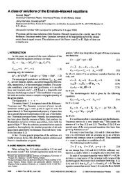
Computations have been performed with a uniform mesh of 128 3 points. Collapse
is found to develop in a flow, which is initially chosen to have random Fourier
harmonics and an exponentially decaying energy spectrum. The flow does not possess
any symmetry. According to the theory of Kuznetsov & Ruban [2], in the
region of collapse vorticity behaves as (t 0 − t) −1 , which is indeed found in computations
(see Fig.1). Their another prediction is confirmed: eigenvalues of the Hessian
‖
∂ 2
∂a i ∂a j
|Ω| −1 ‖ at the point of singularity are non-singular and slightly depend on
time.
Figure 1: |Ω| −1 (vertical axis) as a function of time (horizontal axis).
References
[1] Kuznetsov E.A. & Ruban V.P. (2000). Hamiltonian dynamics of vortex and
magnetic lines in hydrodynamic type systems. Phys. Rev. E, 61, 831–841.
[2] Kuznetsov E.A. & Ruban V.P. (2001). Breaking of vortex lines – a new mechanism
of collapse in hydrodynamics. Submitted.
2