A similarity solution for viscous source flow on a vertical plane

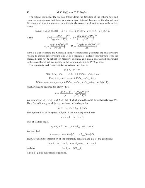
46 B. R. Duffy and H. K. Moffatt
The natural scaling <strong>for</strong> the problem follows from the definition of the volume flux, and
from the assumptions that there is a <strong>viscous</strong>-gravitational balance in the downstream
direction, and that the pressure variations in the transverse direction scale with surface
tension:
where
(x, y, z) X s
(x , δy , εδz), (u, , w) U s
(u , δ , εδw ), p Π s
p , h εδX s
h ,
δ
µQγ
(ρg sin α) X s
/ ,
(ρg sin α) µ Q
ε γX s
/ ,
(ρg sin α) Q
U s
µγX s
/ (ρg sin α) µ Q γ
, Π s
X s
/ .
Here u, and w denote the Cartesian velocity components, p denotes the fluid pressure
relative to atmospheric pressure, and X s
is a measure of distance downstream from the
<strong>source</strong>. X s
need not be defined too precisely, since any length scale selected will be artificial
in the sense that it will not appear in the <strong>solution</strong> (cf. Smith, 1973, p. 276).
The continuity and Navier–Stokes equations then lead to
u x
y
w z
0,
R(uu x
u y
wu z
) δ p x
1δ ε u xx
ε u yy
u zz
,
R(u x
y
w z
) p y
δ ε xx
ε yy
zz
,
Rε(uw x
w y
ww z
) p z
δ ε w xx
ε w yy
ε w zz
(ρg cos αγ) δ X s
,
overbars having dropped <strong>for</strong> clarity; here
R ρU s X ε δ
s
µ
ρ gQ
µ γ X s
/ .
We now take δ 1, ε 1 and R 1 (all of which should be valid <strong>for</strong> sufficiently large X s
).
Then <strong>for</strong> sufficiently small α
π we have, at leading order,
u zz
1, zz
p y
, 0p z
.
This system is to be integrated subject to the boundary conditions
and, at leading order,
u 0 on z0,
u z
z
0 and p h yy
on z h.
We thus find
p h yy
, u hz
z, h yyy
(hz
z).
Then, <strong>for</strong> example, integration of the continuity equation and use of the conditions
w 0 on z0, w uh x
h y
on z h
leads to 3h h x
(h h yyy
) y
,
which is (2.2) is non-dimensional <strong>for</strong>m.