A similarity solution for viscous source flow on a vertical plane

Euro. Jnl of Applied Mathematics (1997), ol. 8,pp. 37–47. 1997 Cambridge University Press 37 

A <strong>similarity</strong> <strong>solution</strong> <strong>for</strong> <strong>viscous</strong> <strong>source</strong> <strong>flow</strong> on a 

vertical plane 

B. R. DUFFY and H. K. MOFFATT 

Department of Mathematics, Uniersity of Strathclyde, Liingstone Tower, 26 Richmond Street, 

Glasgow G1 1XH, UK 

Department of Applied Mathematics and Theoretical Physics, Siler Street, Cambridge CB3 9EW, UK 

(Receied in reised <strong>for</strong>m 29 August 1995) 

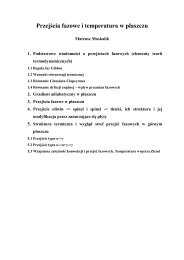
A thin-film approximation is used in an analysis of the <strong>flow</strong> of a thin trickle of <strong>viscous</strong> fluid 

down a near-vertical plane. An approximate <strong>similarity</strong> <strong>solution</strong> is obtained, representing 

essentially a <strong>source</strong> (or sink) <strong>flow</strong>. Several interpretations of the <strong>solution</strong> are discussed. 

1 Introduction 

Problems concerning the ‘draining’ of <strong>viscous</strong> films down inclined surfaces have received 

much attention in the literature. In this paper we use a thin-film approximation to study 

the steady spreading or contraction of <strong>viscous</strong> liquid supplied (at a prescribed rate) on a 

near-vertical plane; gravity may be considered the ‘main’ driving <strong>for</strong>ce, but surface tension 

cannot be neglected. The assumption that the <strong>flow</strong> changes only slowly down the plane then 

leads to an approximate <strong>similarity</strong> <strong>solution</strong> <strong>for</strong> this three-dimensional <strong>viscous</strong> free-surface 

<strong>flow</strong>. Several interpretations of this <strong>solution</strong> are discussed. 

Only steady <strong>flow</strong>s are considered, so that, in particular, any contact lines are fixed; 

difficulties associated with moving contact lines are thereby avoided. (Cf. Davis, 1983, and 

the many references therein.) Unsteady <strong>flow</strong>s have been considered (within a thin-film 

theory) by, <strong>for</strong> example, Huppert (1982), Schwartz (1989), Lister (1992) and Moriarty et al. 

(1991). 

2 The governing equation, and a <strong>similarity</strong> <strong>solution</strong> 

If liquid is supplied (at a prescribed volume flux Q) from a point <strong>source</strong> on an inclined 

plane, then there will be an adjustment region where the trickle widens (from ‘zero’ width) 

until it attains a constant cross section, of non-zero width 2a (say). There will be a similar 

adjustment if the <strong>source</strong> is of small but non-zero width. If the liquid is supplied from a very 

wide <strong>source</strong>, then it is commonly observed that an ‘instability’ occurs, and the stream splits 

into two or more narrower trickles (fingers), each of which is eventually a uni<strong>for</strong>m rivulet. 

Again, there will be adjustment regions where the width of each trickle settles to an 

appropriate value of a (although determination of these values of a is by no means 

straight<strong>for</strong>ward; see, <strong>for</strong> example, Mikielewicz & Moszynski, 1978; Huppert, 1982; 

Schwartz, 1989). 

Smith (1973) has considered the spreading of a trickle from a point <strong>source</strong> on an inclined 

plane in the case when surface tension is negligible. However, when the plane is vertical the

38 B. R. Duffy and H. K. Moffatt 

FIGURE 1. A trickle of fluid emitted on a near-vertical plate. 

effects of surface tension cannot be ignored; we consider this case here, again taking the 

film to be thin and the <strong>flow</strong> to be slow. 

Suppose a thin film of Newtonian liquid, of constant density ρ and viscosity µ, is <strong>flow</strong>ing 

down a plane inclined at an angle α to the horizontal, α being defined such that the liquid 

is on the ‘topside’ of the plane when α 

π and is on the ‘underside’ of the plane when 

α 

π (see Figure 1). We shall take the plane to be vertical or nearly vertical, so that α 

π 

is zero or is small. 

We use Cartesian coordinates Oxyz as in Figure 1, with Ox down a line of greatest slope 

and with Oz normal to the plane. A standard thin-film analysis shows that the (generally 

unsteady) free-surface profile z h(x, y, t) satisfies 

3µh t 

[h(ρgh cos αγ h)]3ρgh h x 

sin α, (2.1) 

where γ denotes the coefficient of surface tension (assumed constant), g denotes the 

acceleration due to gravity, and suffixes denote partial differentiation. 

The case of a rivulet of uni<strong>for</strong>m width is obtained by putting h h(y) and setting to zero 

the term in square brackets in (2.1): 

ρgh cos αγh yy 

constant. 

(cf. Towell & Rothfeld, 1966; Allen & Biggin, 1974). This is to be integrated subject to the 

boundary conditions 

h 0 and htan β 

at y a, 

where a is the semi-width of the trickle, and β 

is the contact angle at the air–liquid–solid 

contact line, taken to be constant. For small α 

π the <strong>solution</strong> is 

h(y) tan β 

2a 

(ay).

A <strong>similarity</strong> <strong>solution</strong> <strong>for</strong> iscous <strong>source</strong> <strong>flow</strong> on a ertical plane 39 

The velocity component down the plane is u (ρg sin α2µ)(2hzz), and the volume flux 

of liquid running down the plane is 

Q a −a h(y) udzdy, ρgsin α 

3µ a 

 

−a 

h dy, 4ρga sin α tan β , 

105µ 

independent of γ (in this approximation). 

In general, liquid issuing from a <strong>source</strong> (whether a point <strong>source</strong> or a distributed <strong>source</strong>) 

will not have this profile, and there will be some sort of adjustment zone be<strong>for</strong>e a constant 

profile can be attained. Smith (1973) has studied this adjustment <strong>for</strong> the case when α is not 

near 

π, with surface tension neglected (at leading order). We, on the other hand, are 

interested in a near-vertical surface, so that α 

π, and surface tension cannot be neglected. 

In the spirit of Smith’s analysis, we seek a steady <strong>solution</strong> <strong>for</strong> which the length scale down 

the plane is much greater than that across the stream, so that h y 

h x 

in general. Then 

equation (21) becomes approximately 

hh yyyy 

3h y 

h yyy 

3(ρg sin αγ) h x 

0. (2.2) 

The self-consistency of this approximation is checked a posteriori (see equations (212) and 

(213)) by verifying that 1 h y 

h x 

<strong>for</strong> the <strong>solution</strong> obtained; a more <strong>for</strong>mal justification 

of the approximation is given in an appendix. 

Here we shall consider <strong>solution</strong>s of (22) that are symmetrical about y 0, or, to be more 

precise, <strong>solution</strong>s <strong>for</strong> which h is even in y. This means that 

h y 

(x,0)0, h yyy 

(x,0)0. (2.3) 

We take the free-surface to meet the plane z 0 in the curves y y e 

(x), which are 

there<strong>for</strong>e three-phase contact lines (the ‘edges’ of the trickle). Then 

h(x, y e 

) 0. (2.4) 

Also, the volume flux of liquid down the plane is approximately 

ρg sin α 

Q 

3µ y e(x) 

h dy, (2.5) 

−y e (x) 

and herein we take Q to be a prescribed constant. 

It is expected that the contact angle β at the (anchored) three-phase lines y y e 

(x) will 

satisfy a restriction of the <strong>for</strong>m β r 

β β a 

, where β r 

and β a 

are constants (the receding and 

advancing contact angles). However, there is no reason to expect β itself to be constant on 

these contact lines (and indeed, simple observations of film-drainage down an inclined 

plane suggest strongly that β will vary quite considerably, at least where the film width 

varies in a downstream direction). Presumably conditions near the lateral contact lines are 

dominated by <strong>viscous</strong> stresses, in which case it is legitimate to assume that the contact angle 

adjusts itself locally to the value dictated by these stresses. There may, of course, be an 

‘inner region’ (perhaps on the scale of intermolecular <strong>for</strong>ces) within which an adjustment 

to the appropriate contact angle takes place; however, the behaviour in such an inner 

region lies outside the scope of the present analysis. We there<strong>for</strong>e leave open the question


of the contact-angle, and merely report a family of free-surface profiles that are consistent 

with (2.2)–(2.5), and <strong>for</strong> which, as we shall see, β is variable. 

We seek a <strong>similarity</strong> <strong>solution</strong> to (2.2) of the <strong>for</strong>m 

h(x, y) f(x) G(η), 

η yy e 

(x), 

so that G(1) 0. 

Substitution of this <strong>for</strong>m of h into (2.2) shows that appropriate f and y e 

are 

f(x) A(cx)m, y e 

(x) (cx)n, m4n1 0, 

where c, A, m and n are constants (a shift of origin having been made, to eliminate any 

additive constant in x). The constancy of Q further implies that 3mn 0, so that 

m 113 and n 313. The constant A( 0) may be chosen freely, and if we make the 

choice A cρg sin α104γ (so that c and A have physical dimensions (length)/ and 

(length)/, respectively) then the equation <strong>for</strong> G(η) is 

GG3GG24(G3ηG) 0, 

i.e. 

G(G24η) constant. 

For the symmetrical <strong>solution</strong>s that we are considering here, we have G 0 when η 0, 

so that the constant of integration is 0. Thus G 24η, and, trivially, the <strong>solution</strong> 

satisfying G(1) 0is 

G(η)(η1)λ(η1), (2.6) 

where λ is some constant. The flux condition gives a relation between c and λ: 

(ρg sin α) c 

Q 

2313γµ G dη, (2.7) 

− 

which reduces to c P(λ) Nγ µ Q, (2.8) 

(ρg sin α) 

where N 235713 3690960 and 

P(λ) λλ 

λ . (2.9) 

This cubic polynomial P(λ) is monotonic in λ, with real root λ ( 1.184). 

Thus, overall we have 

cρg sin α 

h(x, y) 

104γ (cx) −/ G(η), (2.10) 

where η yy e 

(x), y e 

(x) (cx)/, (2.11) 

with G(η) as in (2.6) and with (2.8) holding. The quartic function G(η) essentially gives the 

cross-sectional shape of the trickle at each station x constant; we shall find interpretations 

of the <strong>solution</strong> <strong>for</strong> both positive and negative values of the constant c, valid <strong>for</strong> G(η) 0


FIGURE 2. Cross-sectional profiles given by the function G(η) in equation (2.6), <strong>for</strong> (a) λ 2, 

(b) λ 2, (c) 1 λ 2, (d) λ 1, (e) 0 λ 1, (f) λ 0. In (a) and (c) κ (λ1)/. 

and G(η) 0, respectively (see equation (3.3)). Figure 2 shows the <strong>for</strong>ms of G(η) <strong>for</strong> the 

cases (a) λ 2, (b) λ 2, (c) 1 λ 2, (d) λ 1, (e) 0 λ 1, (f) λ 0. The depth of 

the trickle varies like x−/, and y e 

gives its ‘spread’ as it runs down the plane. (Of course, 

as this is a <strong>similarity</strong> <strong>solution</strong>, the profile is essentially the same at each x-station, merely 

scaled in depth by x−/ and in width by x/. Also at a given x-station the depth and width 

(<strong>for</strong> a given λ) are proportional to Q/ and Q/.) 

We expect the <strong>solution</strong> to be valid if 1 h y 

h x 

in general; evaluation of these 

inequalities at the ‘typical’ value η 1 shows that 

(λ2) ρgc sin α 

cx 52γ / and cx 13 3c / , (2.12) 

which imply essentially that the <strong>solution</strong> can be valid only well away from the origin. Also, 

with the above <strong>for</strong>m <strong>for</strong> h the neglected term ρgh cos α in (2.1) (associated with lateral 

spreading due to gravity) is much smaller than the retained term γh if 

12γ 

cx ρgλ cos α / (2.13) 

(which in fact imposes no restriction in the case when α is exactly π2).

5 

8 


The governing equations (2.2) and (2.4) involve the two length scales 

L 

(γρg sin α)/ and L 

(µQρg sin α)/ (2.14) 

(which are prescribed quantities). There is there<strong>for</strong>e some freedom in choosing nondimensional 

variables. With the scheme 

x kL x , y kL y , y e 

kL y e , h k L h 104, c (kL )/ c , (2.15) 

 

where k N/(L L )/, the <strong>solution</strong> may be written in the <strong>for</strong>m 

 

h (x , y ) 

G(η) 

x /[P(λ)]/ , 

η y , y 

y e P(λ) x / , (2.16) 

e 

with G(η) and P(λ) as in (2.6) and (2.9). The <strong>solution</strong> involves one free parameter, here 

taken to be λ; thus (2.16) represents a family of <strong>solution</strong>s, with parameter λ. 

The analysis is valid <strong>for</strong> both c 0 and c 0, provided that y e 

and h are positive; this 

means that cx 0, that cG 0, and that the η-domain must be chosen such that G(η) is 

of one sign. 

3 Interpretation of the <strong>solution</strong> 

(i) For all cases except case (c) we take η 1 <strong>for</strong> the moment. Case (c) is different in that 

the corresponding interval <strong>for</strong> η is η κ, where κ (λ1)/ (with 1 λ 2); thus, <strong>for</strong> 

example, the integration limits in equation (2.7) <strong>for</strong> case (c) should be κ, rather than 1. 

However, one can show easily that under the change of variables 

η η*(λ*1)/, (λ1)(λ*1) 1, c c*(λ*1)/, y e 

(λ*1)/ y e 

, 

the <strong>solution</strong> <strong>for</strong> case (c) becomes the same as that <strong>for</strong> case (a), with η, λ, c and y e 

replaced 

by η*, λ*, c* and y e 

, and with η* 1. This means that case (c) can be subsumed into case 

(a), and need not be treated separately. 

In all cases, then, the contact angle β(x) atyy e 

and the centre-line depth h 

(x) of the 

liquid are given approximately by 

tan β h (λ2) cρg sin α 

 

y y=ye 

52γ(cx)/ 

(3.1) 

and 

h 

h(x,0) 

(λ1) cρg sin α 

. (3.2) 

104γ(cx)/ 

Note that in this <strong>solution</strong> β varies round the contact line (except when λ 2), and cannot 

be prescribed. (Smith’s <strong>solution</strong> has a similar feature.) It is expected that (3.1) can hold only 

where β r 

β β a 

. 

The condition Q 0 requires that λ λ 

if c 0 and λ λ 

if c 0. In addition the 

conditions h 

0 and 0 tan β ( 1) require that 

either I: c 0, x 0, λ 2, G(η) 0 (cases (a), (b)), 

or II: c 0, x 0, λ 1, G(η) 0 (cases (d), (e), (f)) 

(both of which give Q 0 and h(x, y) 0, as required). 

6 

7 

(3.3)


FIGURE 3. The free-surface shape predicted by the <strong>similarity</strong> <strong>solution</strong> (2.16) in the case λ 0. This is 

of type II, i.e. getting narrower and deeper downstream. The inset shows the cross-sectional profile 

(cf. Figure 2). 

A <strong>solution</strong> of type I describes <strong>flow</strong> (in x 0) from a <strong>source</strong> at x 0, the trickle getting 

wider (like x/) and shallower (like x−/) with distance x down the plane. A <strong>solution</strong> of 

type II describes <strong>flow</strong> (in x 0) into a sink at x 0, the trickle getting narrower and deeper 

down the plane. In type-II <strong>solution</strong>s the lateral contraction can continue only until the 

depth becomes so great (and the contact angle becomes so big) that the fluid ‘spills over’ 

and runs down the plane as a uni<strong>for</strong>m trickle. 

Both types of <strong>solution</strong> are symmetric about the mid-line η 0. As may be seen in Figure 

2, in all cases except (e) the cross section of the trickle (at a fixed x-station) has a single 

maximum, at y 0. In case (e) (<strong>for</strong> which h has the sign of G) the cross section is ‘doublehumped’, 

with maxima at η (λ2)/ and a minimum at η 0. Figures 3, 4 and 5 show 

examples of free-surface profiles <strong>for</strong> three representative values of the parameter λ; the first 

two are of type II and the latter is of type I. 

(ii) Consider now case (c) with 1 λ λ . In the interval κ η 1 we have G(η) 0, 

 

c 0 and x 0; also the limits in the integral in (2.7) become η κ to η 1. The <strong>solution</strong> 

in this interval represents <strong>flow</strong> (into a sink at x 0) of a ‘meandering’ trickle occupying 

κy e 

y y e 

(<strong>for</strong> x 0); the trickle veers away from the line of greatest slope, and gets 

narrower and deeper as the sink is approached. Thus overall the trickle is highly 

asymmetrical in y, even though G is even in η. (There is a similar interpretation <strong>for</strong> the 

<strong>solution</strong> in 1 η κ.) 

(iii) Consider cases (a) and (b) with η κ, so that G(η) 0, c 0, λ 2 and x 0. 

Roughly speaking, these correspond to <strong>flow</strong> of a liquid sheet around the outside of the 

region y e 

y y e 

; thus this region (which, since x 0, gets wider with increasing x) is


FIGURE 4. The free-surface shape in the case λ 0.9. This is of type II. 

FIGURE 5. The free-surface shape in the case λ 3. This is of type I, i.e. getting wider and 

shallower downstream.


a ‘dry patch’, with liquid on either side. However, the liquid sheet extends to y 

outside the dry patch, and the volume flux Q of liquid down the plane is infinite. 

4 Comments 

(i) Simple experiments were per<strong>for</strong>med with large ‘drops’ of syrup on a perspex sheet. 

With the sheet horizontal a drop essentially takes up a static circular equilibrium shape 

(typically of radius 50 mm and depth 5 mm). The sheet is then supported in a vertical 

position, and the liquid allowed to run down under gravity. Of course, the setup does not 

correspond precisely to a constant supply flux, but at least it has the feature that the trickle 

has a lateral contraction as it runs down the plane (somewhat similar to case II(e)) until 

eventually ‘fingers’ <strong>for</strong>m, which become nearly-uni<strong>for</strong>m rivulets running down the line of 

greatest slope. In the contracting zone the <strong>flow</strong> is effectively steady <strong>for</strong> a long time, and the 

trickle cross sections were found to have clear ‘two-humped’ profiles, roughly as in case (e) 

of Figure 2, except that the humps are rather closer to the edges y y e 

(x) of the trickle 

than the figure would suggest; this may imply that the quartic profile in (2.6) is roughly of 

the right <strong>for</strong>m, but is not correct in detail. Also, in the experiments the edges y y e 

(x) 

are only slightly curved (and indeed, in many runs were remarkably straight); in terms of 

the theory, this would mean that the parameter c in (2.11) was very small in the 

experiments. 

(ii) The question arises as to the physical significance of the parameter λ, which is left 

undetermined even when conditions (2.3)–(2.5) are satisfied. Different choices <strong>for</strong> λ can 

lead to very different profiles; perhaps a detailed modelling of the contact-line regions 

would determine which of these (if any) is physically sensible. 

(iii) The <strong>solution</strong> herein may be contrasted with that of Smith (1973), namely 

h(x, y) c x−/ G s 

(η), η yy s 

(x), y s 

(x) c x/, G s 

(η) 1η, (4.1) 

where 

4725µ Q 

c 

1024ρ g sin 2α / , 

12005µQ cos α 

c 

36ρg sin α / . 

This <strong>solution</strong> was obtained by neglecting the term γh in comparison with the term 

ρgh cos α in (2.1); clearly, such an approximation is not appropriate when α π2, and the 

<strong>solution</strong> would break down in that case. Note that there is no free parameter (equivalent 

to λ) in (4.1). 

Smith interpreted his <strong>solution</strong> as representing the steady spreading and shallowing of a 

<strong>viscous</strong> trickle emitted from a ‘point’ <strong>source</strong> Q at the origin. The <strong>solution</strong> (4.1) compares 

favourably with results of Schwartz & Michaelides (1988), who solved (2.1) numerically 

(with γ 0), as an initial value problem. (We may also note that, with the choice 

π2 α π and x 0, Smith’s <strong>solution</strong> may instead be interpreted as representing a sink 

<strong>flow</strong> down the underside of an inclined plane, the trickle contracting and deepening towards 

a sink Q at the origin; such a <strong>flow</strong> would presumably be difficult to establish 

experimentally!) 

Appendix: Derivation of equation (2.2) 

The development here parallels that of Smith (1973).


The natural scaling <strong>for</strong> the problem follows from the definition of the volume flux, and 

from the assumptions that there is a <strong>viscous</strong>-gravitational balance in the downstream 

direction, and that the pressure variations in the transverse direction scale with surface 

tension: 

where 

(x, y, z) X s 

(x , δy , εδz), (u, , w) U s 

(u , δ , εδw ), p Π s 

p , h εδX s 

h , 

δ 

µQγ 

(ρg sin α) X s 

/ , 

(ρg sin α) µ Q 

ε γX s 

/ , 

(ρg sin α) Q 

U s 

µγX s 

/ (ρg sin α) µ Q γ 

, Π s 

X s 

/ . 

Here u, and w denote the Cartesian velocity components, p denotes the fluid pressure 

relative to atmospheric pressure, and X s 

is a measure of distance downstream from the 

<strong>source</strong>. X s 

need not be defined too precisely, since any length scale selected will be artificial 

in the sense that it will not appear in the <strong>solution</strong> (cf. Smith, 1973, p. 276). 

The continuity and Navier–Stokes equations then lead to 

u x 

y 

w z 

0, 

R(uu x 

u y 

wu z 

) δ p x 

1δ ε u xx 

ε u yy 

u zz 

, 

R(u x 

y 

w z 

) p y 

δ ε xx 

ε yy 

zz 

, 

Rε(uw x 

w y 

ww z 

) p z 

δ ε w xx 

ε w yy 

ε w zz 

(ρg cos αγ) δ X s 

, 

overbars having dropped <strong>for</strong> clarity; here 

R ρU s X ε δ 

s 

µ 

 

ρ gQ 

µ γ X s 

/ . 

We now take δ 1, ε 1 and R 1 (all of which should be valid <strong>for</strong> sufficiently large X s 

). 

Then <strong>for</strong> sufficiently small α 

π we have, at leading order, 

u zz 

1, zz 

p y 

, 0p z 

. 

This system is to be integrated subject to the boundary conditions 

and, at leading order, 

u 0 on z0, 

u z 

z 

0 and p h yy 

on z h. 

We thus find 

p h yy 

, u hz 

z, h yyy 

(hz 

z). 

Then, <strong>for</strong> example, integration of the continuity equation and use of the conditions 

w 0 on z0, w uh x 

h y 

on z h 

leads to 3h h x 

(h h yyy 

) y 

, 

which is (2.2) is non-dimensional <strong>for</strong>m.


Acknowledgement 

This work was supported by the Science Research Council under grant no. GRA5993.4. 

References 

ALLEN, R.F.&BIGGIN, C. M. (1974) Longitudinal <strong>flow</strong> of a lenticular liquid filament down an 

inclined plane. Phys. Fluids 17, 287–291. 

DAVIS, S. H. (1983) Contact line problems in fluid mechanics. Trans. ASME, J. Appl. Mechanics 50, 

977–982. 

HUPPERT, H. E. (1982) Flow and instability of a <strong>viscous</strong> current down a slope. Nature 300, 427–429. 

LISTER, J. R. (1992) Viscous <strong>flow</strong>s down an inlined plane from point and line <strong>source</strong>s. J. Fluid 

Mechanics 242, 631–653. 

MIKIELEWICZ,J.&MOSZYNSKI, J. R. (1978) An improved analysis of breakdown of thin liquid films. 

Arch. Mech. Stos. 30, 489–500. 

MORIARTY, J. A., SCHWARTZ, L.W.&TUCK, E. O. (1991) Unsteady spreading of thin liquid films 

with small surface tension. Phys. Fluids A 3, 733–742. 

SMITH, P. C. (1973) A <strong>similarity</strong> <strong>solution</strong> <strong>for</strong> slow <strong>viscous</strong> <strong>flow</strong> down an inclined plane. J. Fluid 

Mechanics 58, 275–288. 

SCHWARTZ, L. W. (1989) Viscous <strong>flow</strong>s down an inclined plane: Instability and finger <strong>for</strong>mation. 

Phys. Fluids A 1, 443–445. 

SCHWARTZ, L.W.&MICHAELIDES, E. E. (1988) Gravity <strong>flow</strong> of a <strong>viscous</strong> liquid down a slope with 

injection. Phys. Fluids 31, 2739–2741. 

TOWELL,G.D.&ROTHFELD, L. B. (1966) Hydrodynamics of rivulet <strong>flow</strong>. J. Am. Inst. Chem. Eng 12, 

972–980.

A similarity solution for viscous source flow on a vertical plane

You also want an ePaper? Increase the reach of your titles

Delete template?

Save as template?