An Economic Assessment of Banana Genetic Improvement and ...

BANANA PRODUCTIVITY AND TECHNICAL EFFICIENCY IN UGANDA 121
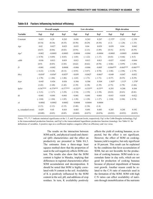
Table 8.6 Factors influencing technical efficiency
Overall sample Low elevation High elevation
Variable
Eq1 Eq2 Eq3 Eq1 Eq2 Eq3 Eq1 Eq2 Eq3
Constant 0.415
0.28
0.263
0.438
0.263
0.267
–2.375*
–2.312
–2.358
(0.54)
(0.36)
(0.35)
(0.50)
(0.29)
(0.30)
(1.3)
(–1.28)
(–1.33)
Age 0.02
0.027
0.025
0.033
0.04
0.039
0.039
0.04
0.042
(0.67)
(0.86)
(0.83)
(0.95)
(1.13)
(1.09)
(0.51)
(0.53)
(0.59)
Age 2 –0.002
–0.0003
–0.0003
–0.0004
–0.004
–0.0004
–0.0003
–0.0003
–0.0004
(–0.70)
(–0.89)
(–0.83)
(–1.05)
(–1.22)
(–1.17)
(0.43)
(–0.46)
(–0.5)
edhh 0.016
0.015
0.019
0.013
0.013
0.015
–0.037
–0.043
–0.044
(0.9)
(0.85)
(1.03)
(0.62)
(0.62)
(0.70)
(–0.86)
(–0.99)
(–1.00)
D –0.001
–0.002
0.0008
–0.006
–0.006
–0.005
–0.064***
–0.065***
–0.061***
(–0.22)
(–0.28)
(0.13)
(–0.95)
(–0.97)
(–0.70)
(–2.88)
(–2.98)
(–2.79)
hhsz –0.054*
–0.056*
–0.055*
–0.059
–0.062*
–0.061*
–0.049
–0.047
–0.032
(–1.78)
(–1.86)
(–1.86)
(–1.65)
(–1.73)
(–1.71)
(–0.57)
(0.55)
(–0.39)
depr 0.443
0.436
0.436
0.506
0.506
0.504
1.505*
1.513*
1.378*
(1.42)
(1.40)
(1.42)
(1.39)
(1.38)
(1.39)
(1.73)
(1.78)
(1.66)
hplot –0.567***
–0.579***
–0.577***
–0.522**
–0.535**
–0.53**
0.293
0.288
0.184
(–3.21)
(–3.27)
(–3.29)
(–2.54)
(–2.59)
(–2.58)
(0.63)
(0.63)
(0.41)
kk –0.001
–0.001
–0.001
–0.001
–0.001
–0.001
–0.015
–0.018
–0.022
(–1.04)
(–1.04)
(–1.03)
(–1.28)
(–1.28)
(–1.27)
(–1.04)
(1.06)
(–0.74)
sk 0.0002
0.0002
0.0002
0.0004
0.0004
0.0004
(1.15)
(1.12)
(1.15)
(1.40)
(1.36)
(1.4)
σ V (standard error) 0.429
0.43
0.414
0.483
0.491
0.483
0.205
0.201
0.192
(0.049)
(0.05)
(0.05)
(0.069)
(0.071)
(0.074)
(0.032)
(0.032)
(0.035)
Notes: ***, **, * indicate statistical significance at the 1, 5, and 10 percent levels, respectively. Eq1 is the Cobb-Douglas technology, Eq2
is the transcendental production function, and Eq3 is the transcendental logarithmic production function (translog). See Table 8.1 for
definitions of variables. A positive sign on a coefficient implies a negative effect on efficiency and vice versa.
The results on the interaction between
SOM and K, and physical (sand) and chemical
(pH) characteristics and the effect on
productivity are presented in Table 8A.3.
The estimates from a three-stage least
squares method show that the proportion of
sand in the soil negatively affects SOM content.
The results also show that the SOM
content is higher in Masaka, implying that
differences in regional characteristics affect
SOM accumulation and decomposition. It
should be noted that SOM is highly correlated
with N content in the soil. Availability
of K is positively influenced by the SOM
content in the soil, pH, and additions of crop
residues. In turn, K availability positively
affects the yield of cooking bananas, as expected,
but the effect is not significant.
However, the effect of SOM on cookingbanana
yield is negative, but only significant
at 10 percent. This result can be explained
by the conditions that favor accumulation of
SOM, but are not favorable for the production
of cooking bananas. SOM tends to accumulate
faster in clay soils, which are not
good for production of cooking bananas
because of physical impediment of banana
root growth. Another reason could be related
to the C:N ratio of materials used in
the formation of the SOM. SOM with high
C:N ratios can affect availability of nutrients
through immobilization of the nutrients