Multiple Description Quantization Via Gram-Schmidt Orthogonalization

1
Multiple Description Quantization Via
Gram-Schmidt Orthogonalization
Jun Chen, Student Member, IEEE, Chao Tian, Student Member, IEEE, Toby Berger, Fellow, IEEE,
Sheila S. Hemami, Senior Member, IEEE
Abstract
The multiple description (MD) problem has received considerable attention as a model of information transmission
over unreliable channels. A general framework for designing efficient multiple description quantization schemes is
proposed in this paper. We provide a systematic treatment of the El Gamal-Cover (EGC) achievable MD rate-distortion
region, and show that any point in the EGC region can be achieved via a successive quantization scheme along with
quantization splitting. For the quadratic Gaussian case, the proposed scheme has an intrinsic connection with the
Gram-Schmidt orthogonalization, which implies that the whole Gaussian MD rate-distortion region is achievable with
a sequential dithered lattice-based quantization scheme as the dimension of the (optimal) lattice quantizers becomes
large. Moreover, this scheme is shown to be universal for all i.i.d. smooth sources with performance no worse than
that for an i.i.d. Gaussian source with the same variance and asymptotically optimal at high resolution. A class
of low-complexity MD scalar quantizers in the proposed general framework also is constructed and is illustrated
geometrically; the performance is analyzed in the high resolution regime, which exhibits a noticeable improvement
over the existing MD scalar quantization schemes.
Index Terms
Gram-Schmidt orthogonalization, lattice quantization, MMSE, multiple description, quantization splitting.
I. INTRODUCTION
In the multiple description problem the total available bit rate is split between two channels and either channel
may be subject to failure. It is desired to allocate rate and coded representations between the two channels, such
that if one channel fails, an adequate reconstruction of the source is possible, but if both channels are available, an
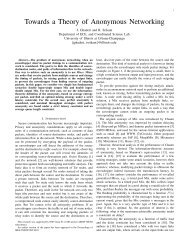
improved reconstruction over the single-channel reception results. The formal definition of the MD problem is as
follows (also see Fig. 1).
Let {X(t)} ∞ t=1 be an i.i.d. random process with X(t) ∼ p(x) for all t. Let d(·, ·) : X × X → [0, d max ] be a
distortion measure.
Jun Chen and Toby Berger are supported in part by NSF Grant CCR-033 0059 and a grant from the National Academies Keck Futures
Initiative (NAKFI). This work has been presented in part at the 39th Annual Conference on Information Sciences and Systems in March 2005.
DRAFT

2
Definition 1.1: The quintuple (R 1 , R 2 , D 1 , D 2 , D 3 ) is called achievable if for all ε > 0, there exist, for n
sufficiently large, encoding functions:
f (n)
i
: X n → C (n)
i
log |C (n)
i | ≤ n(R i + ε) i = 1, 2,
and decoding functions:
g (n)
i
: C (n)
i → X n i = 1, 2
such that for ˆX i = g (n)
i
g (n)
3 : C (n)
1 × C (n)
2 → X n
(f (n)
i (X)), i = 1, 2, and for ˆX 3 = g (n)
3 (f (n)
1 (X), f (n)
2 (X)),
n
1
n E ∑
d(X(t), ˆX i (t)) < D i + ε i = 1, 2, 3.
t=1
The MD rate-distortion region, denoted by Q, is the set of all achievable quintuples.
In this paper the encoding functions f (n)
1 and f (n)
2 are referred to as encoder 1 and encoder 2, respectively.
Similarly, decoding functions g (n)
1 , g (n)
2 and g (n)
3 are referred to as decoder 1, decoder 2, and decoder 3, respectively.
It should be emphasized that in a real system, encoders 1 and 2 are just two different encoding functions of a single
PSfrag replacements
encoder while decoders 1, 2 and 3 are different decoding functions of a single decoder. Alternatively, in the MD
literature decoders 1 and 2 are sometimes referred to as the side decoders because of their positions in Fig. 1, while
decoder 3 is referred to as the central decoder.
X
Encoder 1
Encoder 2
Decoder 1
R 1
Decoder 3
R 2
ˆX 1
ˆX 3
Decoder 2
ˆX 2
Fig. 1.
Encoder and decoder diagram for multiple descriptions.
Early contributions to the MD problem can be found in [1]–[4]. The first general result was El Gamal and Cover’s
achievable region.
Definition 1.2 (EGC region): For random variables U 1 , U 2 and U 3 jointly distributed with the generic source
variable X via conditional distribution p(u 1 , u 2 , u 3 |x), let
Let
R(U 1 , U 2 , U 3 ) = {(R 1 , R 2 ) : R 1 + R 2 ≥ I(X; U 1 , U 2 , U 3 ) + I(U 1 ; U 2 ), R i ≥ I(X; U i ), i = 1, 2} .
Q(U 1 , U 2 , U 3 ) =
{
(R 1 , R 2 , D 1 , D 2 , D 3 ) : (R 1 , R 2 ) ∈ R(U 1 , U 2 , U 3 ), ∃ ˆX i = g i (U i ) with Ed(X, ˆX
}
i ) ≤ D i , i = 1, 2, 3 .
DRAFT

3
The EGC region 1 is then defined as
⎛
Q EGC = conv ⎝
⋃
⎞
Q(U 1 , U 2 , U 3 ) ⎠ ,
p(u 1,u 2,u 3|x)
where conv(S) denotes the convex hull of S for any set S in the Euclidean space.
It was proved in [5] that Q EGC ⊆ Q. Ozarow [3] showed that Q EGC = Q for the quadratic Gaussian source.
Ahlswede [6] showed that the EGC region is also tight for the “no excess sum-rate” case. Zhang and Berger [7]
constructed a counterexample for which Q EGC Q. Further results can be found in [8]–[14]. The MD problem
has also been generalized to the n-channel case [15], [16], but even the quadratic Gaussian case is far from being
completely understood. The extension of the MD problem to the distributed source coding scenario has been
considered in [17], [18], where the problem is again widely open.
The first constructive method to generate multiple descriptions is the multiple description scalar quantization
(MDSQ), which was proposed by Vaishampayan [19], [20]. The key component of this method is the index
assignment, which maps an index to an index pair as the two descriptions. However, the design of the index
assignment turns out to be a difficult problem. Since optimal solution cannot be found efficiently, Vaishampayan
[19] provided several heuristic methods to construct balanced index assignments which are not optimal but likely
to perform well. The analysis of this class of balanced quantizers reveals that asymptotically (in rate) it is 3.07 dB
away from the rate-distortion bound [21] in terms of central and side distortion product, when a uniform central
quantizer is used; this granular distortion gap can be reduced by 0.4 dB when the central quantizer cells are better
optimized [22]. The design of balanced index assignment was recently more thoroughly addressed in [23] from an
algorithm perspective, and the index assignments for more than two description appeared in [24]. Other methods
have also been proposed to optimize the index assignments [25], [26].
The framework of MDSQ was later extended to multiple description lattice vector quantization (MDLVQ) for
balanced descriptions in [27] and for the asymmetric case in [28]. The design relies heavily on the choice of
lattice/sublattice structure to facilitate the construction of index assignments. The analysis on these quantizers shows
that the constructions are high-resolution optimal in asymptotically high dimensions; however, in lower dimension,
optimization of the code-cells can also improve the high-resolution performance [29][30]. The major difficulty in
constructing both MDSQ and MDLVQ is to find good index assignments, and thus it would simplify the overall
design significantly if the component of index assignment can be eliminated altogether.
Frank-Dayan and Zamir [31] proposed a class of MD schemes which use entropy-coded dithered lattice quantizers
(ECDQs). The system consists of two independently dithered lattice quantizers as the two side quantizers, with a
possible third dithered lattice quantizer to provide refinement information for the central decoder. It was found that
even with the quadratic Gaussian source, this system is only optimal in asymptotically high dimensions for the
1 The form of the EGC region here is slightly different from the one given in [5], but it is straightforward to show they are equivalent. g 3 (U 3 )
can be also replaced by a function of (U 1 , U 2 , U 3 ), say ˜g(U 1 , U 2 , U 3 ), but the resulting Q EGC is still the same because for any (U 1 , U 2 , U 3 )
jointly distributed with X, there exist (U 1 , U 2 , Ũ3) with Ũ3 = (U 1 , U 2 , U 3 ) such that ˜g 3 (U 1 , U 2 , U 3 ) = g 3 (Ũ3).
DRAFT

4
degenerate cases such as successive refinement and the “no excess marginal-rate” case, but not optimal in general.
The difficulty lies in generating dependent quantization errors of two side quantizers to simulate the Gaussian
multiple description test channel. Several possible improvements were provided in [31], but the problem remains
unsolved.
The method of MD coding using correlating transforms was first proposed by Orchard, Wang, Vaishampayan, and
Reibman [32], [33], and this technique has then been further developed in [34] and [35]. However, the transformbased
approach is mainly designed for vector sources, and it is most suitable when the redundancy between the
descriptions is kept relatively low.
In this paper we provide a systematic treatment of the El Gamal-Cover (EGC) achievable MD rate-distortion
region and show it can be decomposed into a simplified-EGC (SEGC) region and an superimposed refinement
operation. Furthermore, any point in the SEGC region can be achieved via a successive quantization scheme along
with quantization splitting. For the quadratic Gaussian case, the MD rate-distortion region is the same as the SEGC
region, and the proposed scheme has an intrinsic connection with the Gram-Schmidt orthogonalization method.
Thus we use single-description ECDQs, with independent subtractive dithers as building blocks for this MD coding
scheme, by which the difficulty of generating dependent quantization errors is circumvented. Analytical expressions
for the rate-distortion performance of this system are then derived for general sources, and compared to the optimal
rate regions at both high and low lattice dimensions.
The proposed scheme is conceptually different from those in [31], and it can achieve the whole Gaussian MD
rate-distortion region as the dimension of the (optimal) lattice quantizers becomes large, unlike the method proposed
in [31]. From a construction perspective, the new MD coding system can be realized by 2-3 conventional lattice
quantizers along with some linear operations, and thus it is considerably simpler than MDSQ and MDLVQ by
removing the index assignment and the reliance on the lattice/sublattice structure. Though the proposed coding
scheme suggests many possible implementations of practical quantization methods, the focus of this article is on the
information theoretic framework; thus instead of providing detailed designs of quantizers, a geometric interpretation
of the scalar MD quantization scheme is given as an illustration to connect the information theoretic description of
coding scheme and its practical counterpart.
The remainder of this paper is divided into 6 sections. In Section II, ECDQ and the Gram-Schmidt orthogonalization
method are breifly reviewed and a connection between the successive quantization scheme and the
Gram-Schmidt orthogonalization method is established. In Section III we present a systematic treatment of the
EGC region and show the sufficiency of a successive quantization scheme along with quantization splitting. In
Section IV the quadratic Gaussian case is considered in more depth. In Section V the proposed scheme based on
ECDQ is shown to be universal for all i.i.d. smooth sources with performance no worse than that for an i.i.d.
Gaussian source with the same variance and asymptotically optimal at high resolution. A geometric interpretation
of the scalar MD quantization scheme in our framework is given in Section VI. Some further extensions are
suggested in Section VII, which also serves as the conclusion. Throughout, we use boldfaced letters to indicate
(n-dimensional) vectors, capital letters for random objects, and small letters for their realizations. For example, we
DRAFT

5
let X = (X(1), · · · , X(n)) T and x = (x(1), · · · , x(n)) T .
II. ENTROPY-CODED DITHERED QUANTIZATION AND GRAM-SCHMIDT ORTHOGONALIZATION
In this section, we first give a brief review of ECDQ, and then explain the difficulty of applying ECDQ directly
to the MD problem. As a method to resolve this difficulty, the Gram-Schmidt orthogonalization is introduced and a
connection between the sequential (dithered) quantization and the Gram-Schmidt orthogonalization is established.
The purpose of this section is two-fold: The first is to review related results on ECDQ and the Gram-Schmidt
orthogonalization and show their connection, while the second is to explicate the intuition that motivated this work.
A. Review of Entropy-Coded Dithered Quantization
Some basic definitions and properties of ECDQ from [31] are quoted below. More detailed discussion and
derivation can be found in [36]–[39].
An n-dimensional lattice quantizer is formed from a lattice L n . The quantizer Q n (·) maps each vector x ∈ R n
into the lattice point l i ∈ L n that is nearest to x. The region of all n-vectors mapped into a lattice point l i ∈ L n
is the Voronoi region
V (l i ) = {x ∈ R n : ||x − l i || ≤ ||x − l j ||, ∀j ≠ i} .
The dither Z is an n-dimensional random vector, independent of the source, and uniformly distributed over the
basic cell V 0 of the lattice which is the Voronoi region of the lattice point 0. The dither vector is assumed to be
available to both the encoder and the decoder. The normalized second moment G n of the lattice characterizes the
second moment of the dither vector
1
n E||Z||2 = G n V 2/n ,
where V denotes the volume of V 0 . Both the entropy encoder and the decoder are conditioned on the dither sample
Z; furthermore, the entropy coder is assumed to be ideal. The lattice quantizer with dither represents the source
vector X by the vector W = Q n (X + Z) − Z. The resulting properties of the ECDQ are as follows.
1) The quantization error vector W − X is independent of X and is distributed as −Z. In particular, the
mean-squared quantization error is given by the second moment of the dither, independently of the source
distribution, i.e.,
1
n E||W − X||2 = 1 n E||Z||2 = G n V 2/n .
2) The coding rate of the ECDQ is equal to the mutual information between the input and output of an additive
noise channel Y = X + N, where N, the channel’s noise, has the same probability density function as −Z
(see Fig. 2) ,
H(Q n (X + Z)|Z) = I(X; Y) = h(Y) − h(N).
DRAFT

6
PSfrag replacements
3) For optimal lattice quantizers, i.e., lattice quantizers with the minimal normalized second moment G n , the
autocorrelation of the quantizer noise is “white” , i.e., EZZ T = σ 2 I n where I n is the n × n identity matrix,
σ 2 = G opt
n
V 2/n is the second moment of the lattice, and
∫
G opt
n
= min
Q n(·)
V 0
||x|| 2 dx
nV 1+ 2 n
is the minimal normalized second moment of an n-dimensional lattice.
X
R
Q n (·) E ∼
D
Z
ECDQ
−Z
N = −Z
X
Y
Fig. 2.
ECDQ and its equivalent additive-noise channel.
Consider the following problem to motivate the general result. Suppose a quantization system is needed with
input X 1 and outputs (X 2 , · · · , X M ) such that the quantization errors X i − X 1 , i = 2, · · · , M, are correlated with
each other in a certain predetermined way, but are uncorrelated with X 1 . Seemingly, M − 1 quantizers may be
used, each with X 1 as the input and X i as the output for some i, i = 2, · · · , M. By property 1) of ECDQ, if
dithers are introduced, the quantization errors are uncorrelated (actually independent) of the input of the quantizer.
However, it is difficult to make the quantization errors of these M − 1 quantizers correlated in the desired manner.
One may expect it to be possible to correlate the quantization errors by simply correlating the dithers of different
quantizers, but this turns out to be not true as pointed out in [31]. Next, we present a solution to this problem by
exploiting the relationship between the Gram-Schmidt orthogonalization and sequential (dithered) quantization.
B. Gram-Schmidt Orthogonalization
In order to facilitate the treatment, the problem is reformulated in an equivalent form: Given X1
M with an arbitrary
covariance matrix, construct a quantization system with ˜X 1 as the input and ( ˜X 2 , · · · , ˜X M ) as the outputs such
that the covariance matrices of X1 M and ˜X 1 M are the same.
DRAFT

7
Let H s denote the set of all finite-variance, zero-mean, real scalar random variables. It is well known [40], [41]
that H s becomes a Hilbert space under the inner product mapping
The norm induced by this inner product is
〈X, Y 〉 = E(XY ) : H s × H s → R.
‖X‖ 2 = 〈X, X〉 = EX 2 .
For X M 1 = (X 1 , · · · , X M ) T with X i ∈ H s , i = 1, · · · , M, the Gram-Schmidt orthogonalization can be used to
construct an orthogonal basis B M 1 = (B 1 , · · · , B M ) T for X M 1 . Specifically, the Gram-Schmidt orthogonalization
proceeds as follows:
Note:
E(X iB j)
EB 2 j
B 1 = X 1 ,
∑i−1
B i = X i −
j=1
∑i−1
= X i −
j=1
〈X i , B j 〉
‖B j ‖ 2 B j
E(X i B j )
EBj
2 B j , i = 2, · · · , M.
can assume any real number if B j = 0. Alternatively, B M 1 can also be computed using the
method of linear estimation. Let K X m
1
denote the covariance matrix of (X 1 , · · · , X m ) T and let K XmX m−1
1
E[X m (X 1 , · · · , X m−1 ) T ], then
Here K i−1 ∈ R 1×(i−1) is a row vector satisfying K i−1 K X
i−1
1
B 1 = X 1 , (1)
B i = X i − K i−1 X i−1
1 , i = 2, · · · , M. (2)
= K XiX i−1 . When K
1
X
i−1
1
=
is invertible, K i−1 is
uniquely given by K XiX i−1 K −1 . The product K
1 X i−1
i−1 X1 i−1 is the linear MMSE estimate of X i given X1 i−1 , and
1
is its corresponding linear MMSE estimation error.
EB 2 i
The Gram-Schmidt orthogonalization is closely related to the LDL T factorization. That is, if all leading minors
of K X M
1
are nonzero, then there exists a unique factorization such that K X M
1
= LDL T , where D is diagonal, and
L is lower triangular with unit diagonal. Specifically, D = diag { ‖B 1 ‖ 2 , · · · , ‖B M ‖ 2} and
⎛
⎞
1
〈X 2,B 1〉
‖B 1‖
1
2 〈X
L =
3,B 1〉 〈X 3,B 2〉
‖B 1‖ 2 ‖B 2‖
1
.
2 ⎜
⎝
.
.
.
. ..
⎟
⎠
〈X L,B 1〉 〈X L,B 2〉 〈X L,B 3〉
‖B 1‖ 2 ‖B 2‖ 2 ‖B 3‖
· · · 1
2
B M 1 = L −1 X M 1 is sometimes referred to as the innovation process [40].
DRAFT

8
In the special case in which X M 1 are jointly Gaussian, the elements of B M 1 are given by
B 1 = X 1 ,
B i = X i − E(X i |X1 i−1 )
∑i−1
= X i − E(X i |B j ), i = 2, · · · , M,
j=1
and B M 1 are zero-mean, independent and jointly Gaussian. Moreover, since X i 1 is a deterministic function of
B1, i it follows that Bi+1 M is independent of Xi 1, for i = 1, · · · , M − 1. Note: For i = 2, · · · , M, E(X i |X1 i−1 ) (or
∑ i−1
j=1 E(X i|B j )) is a sufficient statistic 2 for estimation of X i from X1 i−1 (or B1 i−1 ); E(X i |X1 i−1 ) (or ∑ i−1
j=1 E(X i|B j ))
also is the MMSE estimate of X i given X i−1
1 (or B i−1
1 ) and EB 2 i is the MMSE estimation error.
We now show that one can construct a sequential quantization system with X 1 as the input to generate a zeromean
random vector ˜X M 1 = ( ˜X 1 , ˜X 2 , · · · , ˜X M ) T whose covariance matrix is also K X M
1
. Let X M 1 be a zero-mean
random vector with covariance matrix K X M
1
. By (1) and (2), it is true that
X 1 = B 1 , (3)
X i = K i−1 X1 i−1 + B i , i = 2, · · · , M. (4)
√
Assume that B i ≠ 0 for i = 2, · · · , M. Let Q i,1 (·) be a scalar lattice quantizer with step size ∆ i = 12EBi+1 2 ,
i = 1, 2, · · · , M − 1. Let the dither Z i ∼ U(−∆ i /2, ∆ i /2) be a random variable uniformly distributed over the
basic cell of Q i,1 , i = 1, 2, · · · , M − 1. Note: the second subscript n of Q i,n denotes the dimension of the lattice
quantizer. In this case n = 1, so it is a scalar quantizer.
Suppose (X 1 , Z 1 , · · · , Z M−1 ) are independent. Define
˜X 1 = X 1 ,
By property 2) of the ECDQ, we have
where N i ∼ U(∆ i /2, ∆ i /2) with EN 2 i
˜X i = Q i−1,1
(K i−1 ˜Xi−1 1 + Z i−1
)
− Z i−1 , i = 2, · · · , M.
˜X 1 = X 1 , (5)
˜X i = K i−1 ˜Xi−1 1 + N i , i = 2, · · · , M, (6)
= EB2 i+1 , i = 1, · · · , M − 1, and (X 1, N 1 , · · · , N M ) are independent. By
comparing (3), (4) and (5), (6), it is straightforward to verify that X M 1 and ˜X M 1 have the same covariance matrix.
Since EB 2 i (i = 2, · · · , M) are not necessarily the same, it follows that the quantizers Q i,1(·) (i = 1, · · · , M −1)
are different in general. But by incorporating linear pre- and post-filters [38], all these quantizers can be made
identical. Specifically, given a scalar lattice quantizer Q 1 (·) with step size ∆, let the dither Z i ′ ∼ U(−∆/2, ∆/2) be
2 Actually, E(X i |X i−1
1 ) (or ∑ i−1
j=1 E(X i|B j )) is a minimal sufficient statistic; i.e., E(X i |X i−1
1 ) (or ∑ i−1
j=1 E(X i|B j )) is a function of
every other sufficient statistic f(X i−1
1 ) (or f(B i−1
1 )).
DRAFT

9
a random variable uniformly distributed over the basic cell of Q 1 , i = 1, 2, · · · , M−1. Suppose (X 1 , Z ′ 1, · · · , Z ′ M−1 )
are independent. Define
√
where a i = ±
X 1 = X 1 ,
[ ( ) ]
1
X i = a i−1 Q 1 K i−1 X i−1
1 + Z i−1
′ − Z i−1
′ , i = 2, · · · , M,
a i−1
12EBi+1
2
∆
, i = 1, 2, · · · , M − 1. By property 2) of the ECDQ, it is again straightforward to verify
2
that X M 1 and X M 1 have the same covariance matrix. Essentially by introducing the prefilter
1
a i
a i , the quantizer Q 1 (·) is converted to the quantizer Q i,1 (·) for which
Q i,1 (x) = a i Q 1 ( x a i
).
and the postfilter
This is referred to as the shaping [37] of the quantizer Q 1 (·) by a i . In the case where ∆ 2 = 12, we have E(Z ′ i )2 = 1,
i = 1, · · · , M − 1, and the constructed sequential (dithered) quantization system can be regarded as a simulation
of Gram-Schmidt orthonormalization.
If B i = 0 for some i, then ˜X i = K ˜Xi−1
i−1 1 (or X i = K i−1 X i−1
1 ) and therefore no quantization operation is
needed to generate ˜X i−1
i (or X i ) from ˜X 1 (or X i−1
1 ).
The generalization of the correspondence between the Gram-Schmidt orthogonalization and the sequential (dithered)
quantization to the vector case is straightforward; see Appendix I.
III. SUCCESSIVE QUANTIZATION AND QUANTIZATION SPLITTING
In this section, an information-theoretic analysis of the EGC region is provided. Two coding schemes, namely
successive quantization and quantization splitting, are subsequently introduced. Together with Gram-Schmidt orthogonalization,
they are the main components of the quantization schemes that will be presented in the next two
sections.
A. An information theoretic analysis of the EGC region
Rewrite R(U 1 , U 2 , U 3 ) in the following form:
R(U 1 , U 2 , U 3 ) = {(R 1 , R 2 ) : R 1 + R 2 ≥ I(X; U 1 , U 2 ) + I(U 1 ; U 2 ) + I(X; U 3 |U 1 , U 2 ), R i ≥ I(X; U i ), i = 1, 2} .
Without loss of generality, assume that X → U 3 → (U 1 , U 2 ) form a Markov chain since otherwise U 3 can be
replaced by Ũ3 = (U 1 , U 2 , U 3 ) without affecting the rate and distortion constraints. Therefore U 3 can be viewed as
a fine description of X and (U 1 , U 2 ) as coarse descriptions of X. The term I(X, U 3 |U 1 , U 2 ) is the rate used for
the superimposed refinement from the pair of coarse descriptions (U 1 , U 2 ) to the fine description U 3 ; in general,
this refinement rate is split between the two channels. Since description refinement schemes have been studied
extensively in the multiresolution or layered source coding scenario and are well-understood, this operation can be
separated from other parts of the EGC scheme.
DRAFT

10
Definition 3.1 (SEGC region): For random variables U 1 and U 2 jointly distributed with the generic source
variable X via conditional distribution p(u 1 , u 2 |x), let
R(U 1 , U 2 ) = {(R 1 , R 2 ) : R 1 + R 2 ≥ I(X; U 1 , U 2 ) + I(U 1 ; U 2 ), R i ≥ I(X; U i ), i = 1, 2} .
Let
{
Q(U 1 , U 2 ) = (R 1 , R 2 , D 1 , D 2 , D 3 ) : (R 1 , R 2 ) ∈ R(U 1 , U 2 ), ∃ ˆX 1 = g 1 (U 1 ), ˆX 2 = g 2 (U 2 ), ˆX 3 = g 3 (U 1 , U 2 )
}
with Ed(X, ˆX i ) ≤ D i , i = 1, 2, 3 .
The SEGC region is defined as
⎛
⎞
Q SEGC = conv ⎝
⋃
Q(U 1 , U 2 ) ⎠ .
p(u 1,u 2|x)
The SEGC region first appeared in [1] and was attributed to El Gamal and Cover. It was shown in [7] that
Q SEGC ⊆ Q EGC .
Using the identity
I(A; BC) = I(A; B) + I(A; C) + I(B; C|A) − I(B; C),
R(U 1 , U 2 ) can be written as
R(U 1 , U 2 ) = {(R 1 , R 2 ) : R 1 + R 2 ≥ I(X; U 1 ) + I(X; U 2 ) + I(U 1 ; U 2 |X), R i ≥ I(X; U i ), i = 1, 2} .
The typical shape of R(U 1 , U 2 ) is shown in Fig. 3.
R 2
V 1
V 2
PSfrag replacements
R 1
Fig. 3. The shape of R(U 1 , U 2 ).
It is noteworthy that R(U 1 , U 2 ) resembles Marton’s achievable region [42] for a two-user broadcast channel. This
is not surprising since the proof of the EGC theorem relies heavily on the results in [43] which were originally for a
simplified proof of Marton’s coding theorem for the discrete memoryless broadcast channel. Since the corner points
of Marton’s region can be achieved via a relatively simple coding scheme due to Gel’fand and Pinsker [44], which
for the Gaussian case becomes Costa’s dirty paper coding [45], it is natural to conjecture that simple quantization
DRAFT

11
schemes may exist for the corner points of R(U 1 , U 2 ). This conjecture turns out to be correct as will be shown
below.
Since I(U 1 ; U 2 |X) ≥ 0, the sum-rate constraint in R(U 1 , U 2 ) is always effective. Thus
{(R 1 , R 2 ) : R 1 + R 2 = I(X; U 1 ) + I(X; U 2 ) + I(U 1 ; U 2 |X), R i ≥ I(X; U i ), i = 1, 2}
will be called the dominant face of R(U 1 , U 2 ). Any rate pair inside R(U 1 , U 2 ) is inferior to some rate pair on the
dominant face in terms of compression efficiency. Hence, in searching for the optimal scheme, attention can be
restricted to rate pairs on the dominant face without loss of generality. The dominant face of R(U 1 , U 2 ) has two
vertices V 1 and V 2 . Let (R 1 (V i ), R 2 (V i )) denote the coordinates of vertex V i , i = 1, 2, then
V 1 : R 1 (V 1 ) = I(X; U 1 ), R 2 (V 1 ) = I(X, U 1 ; U 2 );
V 2 : R 1 (V 2 ) = I(X, U 2 ; U 1 ), R 2 (V 2 ) = I(X; U 2 ).
The expressions of these two vertices directly lead to the following successive quantization scheme. By symmetry,
we shall only consider V 1 .
B. Successive Quantization Scheme
The successive quantization scheme is given as follows:
1) Codebook Generation: Encoder 1 independently generates 2 n[I(X;U1)+ɛ1] codewords {U 1 (j)} 2n[I(X;U 1 )+ɛ 1 ]
j=1 according
to the distribution ∏ p(u 1 ). Encoder 2 independently generates 2 n[I(X,U1;U2)+ɛ2] codewords {U 2 (k)} 2n[I(X,U 1 ;U 2 )+ɛ 2 ]
k=1
according to the distribution ∏ p(u 2 ).
2) Encoding Procedure: Given X, encoder 1 finds the codeword U 1 (j ∗ ) such that U 1 (j ∗ ) is strongly typical
with X. Then encoder 2 finds the codeword U 2 (k ∗ ) such that U 2 (k ∗ ) is strongly typical with X and U 1 (j ∗ ).
Index j ∗ is transmitted through channel 1 and index k ∗ is transmitted through channel 2.
3) Reconstruction: Decoder 1 reconstructs ˆX 1 with ˆX 1 (t) = g 1 (U 1 (j ∗ , t)). Decoder 2 reconstructs ˆX 2 with
ˆX 2 (t) = g 2 (U 2 (k ∗ , t)). Decoder 3 reconstructs ˆX 3 with ˆX 3 (t) = g 3 (U 1 (j ∗ , t), U 2 (k ∗ , t)). Here, U 1 (j ∗ , t)
and U 2 (k ∗ , t) are the t-th entries of U 1 (j ∗ ) and U 2 (k ∗ ), respectively, t = 1, 2, · · · , n.
It can be shown rigorously that
1
n∑
Ed(X i (t),
n
i (t))
t=1
≤ Ed(X, g i (U i )) + ɛ 2+i , i = 1, 2,
1
n∑
Ed(X 3 (t),
n
3 (t)) ≤ Ed(X, g 3 (U 1 , U 2 )) + ɛ 5
t=1
as n goes to infinity and ɛ i (i = 1, 2, · · · , 5) can be made arbitrarily close to zero. The proof is conventional and
thus is omitted.
For this scheme, encoder 1 does the encoding first and then encoder 2 follows. The main complexity of this
scheme resides in encoder 2, since it needs to construct a codebook that covers the (X, U 1 )-space instead of just the
X-space. Observe that, if a function f(X, U 1 ) = V can be found such that V is a sufficient statistic for estimation
DRAFT

12
U 2 from (X, U 1 ), i.e., (X, U 1 ) → V → U 2 form a Markov chain 3 , then
I(X, U 1 ; U 2 ) = I(V ; U 2 ).
The importance of this observation is that encoder 2 then only needs to construct a codebook that covers the V-
space instead of the (X, U 1 )-space. This is because the Markov lemma [46] implies that if U 2 is jointly typical
with V, then U 2 is jointly typical with (X, U 1 ) with high probability. This observation turns out to be crucial for
the quadratic Gaussian case.
We point out that the successive coding structure associated with the corner points of R(U 1 , U 2 ) is not a special
case in network information theory. Besides its resemblance to the successive Gel’fand-Pinsker coding structure
associated with the corner points of the Marton’s region previously mentioned, other noteworthy examples include
the successive decoding structure associated with the corner points of the Slepian-Wolf region [47] (and more
generally, the Berger-Tung region [46], [48], [49]) and the corner points of the capacity region of the memoryless
multiaccess channel [50], [51].
C. Successive Quantization Scheme with Quantization Splitting
A straightforward method to achieve an arbitrary rate pair on the dominant face of R(U 1 , U 2 ) is timesharing of
coding schemes that achieve the two vertices. However, such a scheme requires four quantizers in general. Instead,
the scheme based on quantization splitting introduced below needs only three quantizers. Before presenting it, we
shall first prove the following theorem.
Theorem 3.1: For any rate pair (R 1 , R 2 ) on the dominant face of R(U 1 , U 2 ), there exists a random variable U 2
′
with (X, U 1 ) → U 2 → U 2 ′ such that
R 1 = I(X, U 2; ′ U 1 ),
R 2 = I(X; U 2) ′ + I(X, U 1 ; U 2 |U 2).
′
Similarly, there exists a random variable U 1 ′ with (X, U 2 ) → U 1 → U 1 ′ such that
R 1 = I(X, U 1) ′ + I(X, ˆX 2 ; U 1 |U 1),
′
R 2 = I(X, U 1; ′ U 2 ).
Before proceeding to prove this theorem, we make the following remarks.
• By the symmetry between the two forms, only the statement regarding the first form needs to be proved.
• Since (X, U 1 ) → U 2 → U 2 ′ form a Markov chain, if U 2 ′ is independent of U 2 , then it must be independent of
(X, U 1 , U 2 ) altogether 4 . Then in this case,
R 1 = I(X; U 1 ), R 2 = I(X, U 1 ; U 2 ),
3 Such a function f(·, ·) always exists provided |V| ≥ |X ||U 1 |.
4 This is because p(x, u 1 , u 2 |u ′ 2 ) = p(u 2|u ′ 2 )p(x, u 1|u 2 , u ′ 2 ) = p(u 2)p(x, u 1 |u 2 ) = p(x, u 1 , u 2 ).
DRAFT

13
which are the coordinates of V 1 .
• At the other extreme, letting U ′ 2 be U 2 gives
which are the coordinates of V 2 .
Proof:
R 1 = I(X, U 2 ; U 1 ), R 2 = I(X, U 2 ),
First construct a class of transition probabilities 5 p ɛ (u ′ 2|u 2 ) indexed by ɛ such that I(U; U ′ 2) varies
continuously from 0 to H(U 2 ) as ɛ changes from 0 to 1, with (X, U 1 ) → U 2 → U ′ 2 holding for all the members
of this class. It remains to show that
This is indeed true since
R 1 + R 2 = I(X, U 1 ) + I(X; U 2 ) + I(U 1 ; U 2 |X).
R 1 + R 2 = I(X, U ′ 2; U 1 ) + I(X; U ′ 2) + I(X, U 1 ; U 2 |U ′ 2)
= I(X, U ′ 2; U 1 ) + I(X; U ′ 2) + I(X; U 2 |U ′ 2) + I(U 1 ; U 2 |X, U ′ 2)
= I(X, U 2 , U ′ 2; U 1 ) + I(X; U 2 , U ′ 2).
By the construction (X, U 1 ) → U 2 → U ′ 2, it follows that
which completes the proof.
I(X, U 2 , U ′ 2; U 1 ) + I(X; U 2 , U ′ 2)
= I(X, U 2 ; U 1 ) + I(X; U 2 )
= I(X, U 1 ) + I(X; U 2 ) + I(U 1 ; U 2 |X),
The successive quantization scheme with quantization splitting is given as follows:
1) Codebook Generation: Encoder 1 independently generates 2 n[I(X,U ′ 2 ;U1)+ɛ′ 1 ] codewords {U 1 (i)} 2n[I(X,U′ 2 ;U 1 )+ɛ′ 1 ]
i=1
according to the marginal distribution ∏ p(u 1 ). Encoder 2 independently generates 2 n[I(X;U ′ 2 )+ɛ′ 2 ] codewords
{U ′ 2(j)} 2n[I(X;U′ 2 )+ɛ′ 2 ]
j=1 according to the marginal distribution ∏ p(u ′ 2). For each codeword U ′ 2(j), encoder 2
independently generates 2 n[I(X,U1;U2|U ′ 2 )+ɛ′ 3 ] codewords {U 2 (j, k)} 2n[I(X,U 1 ;U 2 |U′ 2 )+ɛ′ 3 ]
k=1
according to the conditional
distribution ∏ p(u 2 |U 2(j, ′ t)). Here U 2(j, ′ t) is the t-th entry of U ′ 2(j)
t
2) Encoding Procedure: Given X, encoder 2 finds the codeword U ′ 2(j ∗ ) such that U ′ 2(j ∗ ) is strongly typical
with X. Then encoder 1 finds the codeword U 1 (i ∗ ) such that U 1 (i ∗ ) is strongly typical with X and U ′ 2(j ∗ ).
Finally, encoder 2 finds the codeword U 2 (j ∗ , k ∗ ) such that U 2 (j ∗ , k ∗ ) is strongly typical with X, U 1 (i ∗ )
and U ′ 2(j ∗ ). Index i ∗ is transmitted through channel 1. Indices j ∗ and k ∗ are transmitted through channel 2.
3) Reconstruction: Decoder 1 reconstructs ˆX 1 with ˆX 1 (t) = g 1 (U 1 (i ∗ , t)). Decoder 2 reconstructs ˆX 2 with
ˆX 2 (t) = g 2 (U 2 (j ∗ , k ∗ , t)). Decoder 3 reconstructs ˆX 3 with ˆX 3 (t) = g 3 (U 1 (i ∗ , t), U 2 (j ∗ , k ∗ , t)). Here U 1 (i ∗ , t)
is the t-th entry of U 1 (i ∗ ) and U 2 (j ∗ , k ∗ , t) is the t-th entry of U 2 (j ∗ , k ∗ ), t = 1, 2, · · · , n.
5 There are many ways to construct such a class of transition probabilities. For example, we can let p 0 (u ′ 2 |u 2) = p(u ′ 2 ), p 1(u ′ 2 |u 2) =
δ(u 2 , u ′ 2 ), and set pɛ(u′ 2 |u 2) = (1 − ɛ)p 0 (u ′ 2 |u 2) + ɛp 1 (u ′ 2 |u 2). Here δ(u 2 , u ′ 2 ) = 1 if u 2 = u ′ 2 and = 0 otherwise.
DRAFT

14
Again, it can be shown rigorously that
1
n∑
Ed(X i (t),
n
i (t))
t=1
≤ Ed(X, g i (U i )) + ɛ ′ 3+i, i = 1, 2,
1
n∑
Ed(X 3 (t),
n
3 (t)) ≤ Ed(X, g 3 (U 1 , U 2 )) + ɛ ′ 6
t=1
as n goes to infinity and ɛ ′ i (i = 1, 2, · · · , 6) can be made arbitrarily close to zero. The proof is standard, so the
details are omitted.
This approach is a natural generalization of the successive quantization scheme for the vertices of R(U 1 , U 2 ).
U ′ 2 can be viewed as a coarse description of X and U 2 as a fine description of X. The idea of introducing an
auxiliary coarse description to convert a joint coding scheme to a successive coding scheme has been widely
used in the distributed source coding problems [52]–[54]. Similar ideas have also found application in multiaccess
communications [55]–[58].
IV. THE GAUSSIAN MULTIPLE DESCRIPTION REGION
In this section we apply the general results in the preceding section to the quadratic Gaussian case 6 . The Gaussian
MD rate-distortion region is first analyzed to show that Q EGC = Q SEGC in this case. Then, by incorporating
the Gram-Schmidt orthogonalization with successive quantization and quantization splitting, a coding scheme that
achieves the whole Gaussian MD region is presented.
A. An Analysis of the Gaussian MD Region
Let {X G (t)} ∞ t=1 be an i.i.d. Gaussian process with X G (t) ∼ N (0, σX 2 ) for all t. Let d(·, ·) be the squared error
distortion measure. For the quadratic Gaussian case, the MD rate-distortion region was characterized in [3], [5],
[60]. Namely, (R 1 , R 2 , D 1 , D 2 , D 3 ) ∈ Q if and only if
R i ≥ 1 2 log σ2 X
D i
, i = 1, 2,
where
R 1 + R 2 ≥ 1 2 log σ2 X
D 3
+ 1 2 log ψ(D 1, D 2 , D 3 ),
⎧
1, D 3 < D 1 + D 2 − σX
⎪⎨
2 (
σ
ψ(D 1 , D 2 , D 3 ) =
2 X D3
1
D 1D 2
, D 3 >
D 1
+ 1 D 2
− 1
σX
2
(σ ⎪⎩
√ 2 X −D3)2
(σX 2 −D3)2 −[ (σX 2 −D1)(σ2 −D2)−√ , o.w.
X (D 1−D 3)(D 2−D 3)] 2
) −1
The case D 3 < D 1 + D 2 − σ 2 X and the case D 3 > ( 1/D 1 + 1/D 2 − 1/σ 2 X) −1
are degenerate. It is easy to
verify that for any (R 1 , R 2 , D 1 , D 2 , D 3 ) ∈ Q with D 3 < D 1 + D 2 − σ 2 X , there exist D∗ 1 ≤ D 1 , D ∗ 2 ≤ D 2 such that
6 All our results derived under the assumption of discrete memoryless source and bounded distortion measure can be generalized to the
quadratic Gaussian case, using the technique in [59].
DRAFT

15
(R 1 , R 2 , D1, ∗ D2, ∗ D 3 ) ∈ Q and D 3 = D1 ∗ + D2 ∗ − σX 2 . Similarly, for any (R 1, R 2 , D 1 , D 2 , D 3 ) ∈ Q with D 3 >
( ) −1,
1/D1 + 1/D 2 − 1/σX
2 there exist D
∗
3 = ( )
1/D 1 + 1/D 2 − 1/σX
2 −1
< D3 such that (R 1 , R 2 , D 1 , D 2 , D3) ∗ ∈
Q. Henceforth we shall only consider the subregion when ( 1/D 1 + 1/D 2 − 1/σX) 2 −1
≥ D3 ≥ D 1 + D 2 − σX 2 , for
which D 1 , D 2 and D 3 all are effective.
Following the approach in [5], let
U 1 = X G + T 0 + T 1 , (7)
U 2 = X G + T 0 + T 2 , (8)
where (T 1 , T 2 ), T 0 , X are zero-mean, jointly Gaussian and independent, and E(T 1 T 2 ) = −σ T1 σ T2 . Let ˆXG i =
E(X G |U i ) = α i U i (i = 1, 2), and ˆX 3
G = E(X G |U 1 , U 2 ) = β 1 U 1 + β 2 U 2 , where
α i =
β 1 =
β 2 =
σ 2 X
σ 2 X + σ2 T 0
+ σ 2 T i
, i = 1, 2,
σ 2 X σ T 2
(σ T1 + σ T2 )(σ 2 X + σ2 T 0
) ,
σ 2 X σ T 1
(σ T1 + σ T2 )(σ 2 X + σ2 T 0
) .
Set E(X G − ˆX G i )2 = D i , i = 1, 2, 3; then
σ 2 T 0
=
D 3 σX
2
σX 2 − D , (9)
3
With these σ 2 T i
σT 2 D i σX
2
i
=
σX 2 − D −
D 3σX
2
i σX 2 − D , i = 1, 2. (10)
3
(i = 0, 1, 2), it is straightforward to verify that
I(X G ; U i ) = 1 2 log σ2 X + σ2 T 0
+ σ 2 T i
σ 2 T 0
+ σ 2 T i
= 1 2 log σ2 X
D i
i = 1, 2,
I(X G ; U 1 ) + I(X G ; U 2 ) + I(U 1 ; U 2 |X G ) = 1 2 log σ2 X + σ2 T 0
+ σ 2 T 1
σ 2 T 0
+ σ 2 T 1
+ 1 2 log σ2 X + σ2 T 0
+ σ 2 T 2
σ 2 T 0
+ σ 2 T 2
+ 1 2 log (σ2 T 0
+ σ 2 T 1
)(σ 2 T 0
+ σ 2 T 2
)
σ 2 T 0
(σ T1 + σ T2 ) 2
Therefore, we have
= 1 2 log σ2 X
D 3
+ 1 2 log ψ(D 1, D 2 , D 3 ).
R G (U 1 , U 2 ) { (R 1 , R 2 ) : R 1 + R 2 ≥ I(X G ; U 1 ) + I(X G ; U 2 ) + I(U 1 ; U 2 |X G ), R i ≥ I(X G ; U i ), i = 1, 2 }
{
= (R 1 , R 2 ) : R 1 + R 2 ≥ 1 2 log σ2 X
+ 1 D 3 2 log ψ(D 1, D 2 , D 3 ), R i ≥ 1 }
2 log σ2 X
, i = 1, 2 . (11)
D i
Hence for the quadratic Gaussian case,
Q = Q EGC = Q SEGC
DRAFT

16
and there is no need to introduce U 3 (more precisely, U 3 can be represented as a deterministic function of U 1 and
U 2 ).
The coordinates of the vertices V G
1 and V G
2 of R G (U 1 , U 2 ) can be computed as follows.
R 1 (V G
1 ) = 1 2 log σ2 X + σ2 T 0
+ σ 2 T 1
σ 2 T 0
+ σ 2 T 1
= 1 2 log σ2 X
D 1
, (12)
R 2 (V G
1 ) = 1 2 log (σ2 X + σ2 T 0
+ σ 2 T 2
)(σ 2 T 0
+ σ 2 T 1
)
σ 2 T 0
(σ T1 + σ T2 ) 2
and
= 1 2 log D 1
D 3
+ 1 2 log ψ(D 1, D 2 , D 3 ). (13)
R 1 (V G
2 ) = 1 2 log (σ2 X + σ2 T 0
+ σ 2 T 1
)(σ 2 T 0
+ σ 2 T 2
)
σ 2 T 0
(σ T1 + σ T2 ) 2
= 1 2 log D 2
D 3
+ 1 2 log ψ(D 1, D 2 , D 3 ), (14)
R 2 (V G
2 ) = 1 2 log σ2 X + σ2 T 0
+ σ 2 T 2
σ 2 T 0
+ σ 2 T 2
Henceforth we shall assume that for fixed (D 1 , D 2 , D 3 ), σ 2 T i
= 1 2 log σ2 X
D 2
. (15)
(i = 0, 1, 2) are uniquely determined by (9) and
(10), and consequently R G (U 1 , U 2 ) is given by (11). Since only the optimal MD coding scheme is of interest, the
sum-rate R 1 + R 2 should be minimized with respect to the distortion constraints (D 1 , D 2 , D 3 ), i.e., (R 1 , R 2 ) must
be on the dominant face of R G (U 1 , U 2 ). Thus for fixed (D 1 , D 2 , D 3 ),
B. Successive Quantization for Gaussian Source
R 1 + R 2 = 1 2 log σ2 X
D 3
+ 1 2 log ψ(D 1, D 2 , D 3 ). (16)
If we view U 1 , U 2 as two different quantizations of X G and let U 1 − X G and U 2 − X G be their corresponding
quantization errors, then it follows
E[(U 1 − X G )(U 2 − X G )] = E[(T 0 + T 1 )(T 0 + T 2 )]
= σ 2 T 0
− σ T1 σ T2
=
D 3 σX
2
σX 2 − D 3
√ (
D1 σX
2 −
σX 2 − D −
1
D 3σX
2 ) (
D2 σX
2
σX 2 − D 3 σX 2 − D −
D 3σX
2
2 σX 2 − D 3
)
, (17)
which is non-zero unless D 3 = ( 1/D 1 + 1/D 2 − 1/σ 2 X) −1.
The existence of correlation between the quantization
errors is the main difficulty in designing the optimal MD quantization schemes. To circumvent this difficulty, U 1
DRAFT

17
and U 2 can be represented in a different form by using the Gram-Schmidt orthogonalization. It yields that
where
B 1 = X G ,
B 2 = U 1 − E(U 1 |X G ) = U 1 − X G ,
B 3 = U 2 − E(U 2 |X G , U 1 ) = U 2 − a 1 X G − a 2 U 1 ,
a 1 = σ2 T 1
+ σ T1 σ T2
σ 2 T 0
+ σ 2 T 1
, (18)
It can be computed that
a 2 = σ2 T 0
− σ T1 σ T2
σ 2 T 0
+ σ 2 T 1
. (19)
EB 2 2 = σ 2 T 0
+ σ 2 T 1
, (20)
EB 2 3 = σ2 T 0
(σ T1 + σ T2 ) 2
σ 2 T 0
+ σ 2 T 1
. (21)
Now consider the quantization scheme for vertex V G
1 of R G (U 1 , U 2 ) (see Fig. 4). R 1 (V G
1 ) is given by
R 1 (V G
1 ) = I(X G ; U 1 ) = I(X G ; X G + B 2 ). (22)
Since U 2 = E(U 2 |X G , U 1 )+B 3 , where B 3 is independent of (X G , U 1 ), it follows that (X G , U 1 ) → E(U 2 |X G , U 1 ) →
U 2 form a Markov chain. Clearly, E(U 2 |X G , U 1 ) → (X G , U 1 ) → U 2 also form a Markov chain since E(U 2 |X G , U 1 )
is a deterministic function of (X G , U 1 ). These two Markov relationships imply that
and thus
I(X G , U 1 ; U 2 ) = I(E(U 2 |X G , U 1 ); U 2 ),
R 2 (V G
2 ) = I(X G , U 1 ; U 2 )
= I(E(U 2 |X G , U 1 ); U 2 )
= I(a 1 X G + a 2 U 1 ; a 1 X G + a 2 U 1 + B 3 ). (23)
Although the above expressions are all of single letter type, it does not mean that symbol by symbol operations
can achieve the optimal bound. Instead, when interpreting these information theoretic results, one should think of
a system that operates on long blocks. Roughly speaking, (22) and (23) imply that
1) Encoder 1 is a quantizer of rate R 1 (V G
1 ) whose input is X G and output is U 1 . The quantization error is
B 2 = U 1 − X G , which is a zero-mean Gaussian vector with covariance matrix EB 2 2I n .
2) Encoder 2 is a quantizer of rate R 2 (V G
1 ) with input a 1 X G + a 2 U 1 and output U 2 . The quantization error
B 3 = U 2 − a 1 X G − a 2 U 1 is a zero-mean Gaussian vector with covariance matrix EB 2 3I n .
Remarks:
DRAFT

18
1) U 1 (or U 2 ) is not a deterministic function of X G (or a 1 X G + a 2 U 1 ), and for classical quantizers the
quantization noise is generally not Gaussian. Thus strictly speaking, the “noise-adding” components in Fig.
4 are not quantizers in the traditional sense. We nevertheless refer to them as quantizers 7 in this section for
simplicity.
2) U 1 is revealed to decoder 1 and decoder 3, and U 2 is revealed to decoder 2 and decoder 3. Decoder i
PSfrag replacements
approximates X by ˆX i = α i U i , i = 1, 2. Decoder 3 approximates X by ˆX 3 = β 1 U 1 + β 2 U 2 . The rates to
reveal U 1 and U 2 are the rates of description 1 and description 2, respectively.
3) From Fig. 4, it is obvious that the MD quantization for V G
1 is essentially the Gram-Schmidt orthogonalization
of (X G , U 1 , U 2 ). As previously shown in Section II, the Gram-Schmidt orthogonalization can be simulated
by sequential (dithered) quantization. The formal description and analysis of this quantization scheme in the
context of multiple descriptions for general sources will be given in Section V.
B 2
B 3
U 1 ˆX G 1
+
×
X G ×
+ ˆX G 3
β 1 ×
β 2 ×
× + +
U 2
× ˆX G 2
a 1
a 2
α 1
α 2
Fig. 4.
MD quantization scheme for V G
1 .
C. Successive Quantization with Quantization Splitting for Gaussian Source
Now we study the quantization scheme for an arbitrary rate pair (R1 G , R2 G ) on the dominant face of R G (U 1 , U 2 ).
Note that since the rate sum R1 G + R2
G is given by (16), (R1 G , R2 G ) only has one degree of freedom.
Let U 2 ′ = X G +T 0 +T 2 +T 3 , where T 3 is zero-mean, Gaussian and independent of (X G , T 0 , T 1 , T 2 ). It is easy to
verify that (X G , U 1 ) → U 2 → U 2 ′ form a Markov chain. Applying the Gram-Schmidt orthogonalization algorithm
7 This slight abuse of the word “quantizer” can be justified in the context of ECDQ (as we will show in the next section) since the quantization
noise of the optimal lattice quantizer is indeed asymptotically Gaussian; furthermore, the quantization noise is indeed independent of the input
for ECDQ [37].
DRAFT

19
to (X G , U ′ 2, U 1 ), we have
˜B 1 = X,
˜B 2 = U ′ 2 − E(U ′ 2|X G ) = U ′ 2 − X G ,
˜B 3 = U 1 − E(U 1 |X G , U ′ 2) = U 1 − b 1 X G − b 2 U ′ 2,
where
b 1 = σ2 T 2
+ σ 2 T 3
+ σ T1 σ T2
σ 2 T 0
+ σ 2 T 2
+ σ 2 T 3
, (24)
b 2 =
σ 2 T 0
− σ T1 σ T2
σ 2 T 0
+ σ 2 T 2
+ σ 2 T 3
. (25)
The variances of ˜B 2 and ˜B 3 are
E ˜B 2 2 = σ 2 T 0
+ σ 2 T 2
+ σ 2 T 3
, (26)
E ˜B 2 3 = σ2 T 0
(σ T1 + σ T2 ) 2 + σ 2 T 3
(σ 2 T 0
+ σ 2 T 1
)
σ 2 T 0
+ σ 2 T 2
+ σ 2 T 3
. (27)
Since U 1 = E(U 1 2|X G , U ′ 2)+ ˜B 3 , where ˜B 3 is independent of (X G , U ′ 2), it follows that (X G , U ′ 2) → E(U 1 |X G , U ′ 2) →
U 1 form a Markov chain. Clearly, E(U 1 |X G , U ′ 2) → (X G , U ′ 2) → U 1 also form a Markov chain because E(U 1 |X G , U ′ 2)
is determined by (X G , U ′ 2). Thus we have
and this gives
Hence σT 2 3
is uniquely determined by
We also can readily compute
I(X G , U ′ 2; U 1 ) = I(E(U 1 |X G , U ′ 2); U 1 ),
R G 1 = I(X G , U ′ 2; U 1 )
= I(E(U 1 |X G , U ′ 2); U 1 )
= 1 2 log EU 2 1
E ˜B 2 3
= 1 2 log (σ2 X + σ2 T 0
+ σ 2 T 1
)(σ 2 T 0
+ σ 2 T 2
+ σ 2 T 3
)
σ 2 T 0
(σ T1 + σ T2 ) 2 + σ 2 T 3
(σ 2 T 0
+ σ 2 T 1
) .
σT 2 3
= σ2 T 0
(σ T1 + σ T2 ) 2 2 2R1 − (σT 2 0
+ σT 2 2
)(σX 2 + σ2 T 0
+ σT 2 1
)
σX 2 + σ2 T 0
+ σT 2 1
− 2 2R1 (σT 2 0
+ σT 2 . (28)
1
)
R G 2 = I(X G ; U 1 ) + I(X G ; U 2 ) + I(U 1 ; U 2 |X G ) − R G 1
= 1 2 log [σ2 T 0
(σ T1 + σ T2 ) 2 + σ 2 T 3
(σ 2 T 0
+ σ 2 T 1
)](σ 2 X + σ2 T 0
+ σ 2 T 2
)
σ 2 T 0
(σ 2 T 0
+ σ 2 T 2
+ σ 2 T 3
)(σ T1 + σ T2 ) 2 ,
DRAFT

20
R G 1 | σ 2
T3 =0 = 1 2 log (σ2 X + σ2 T 0
+ σ 2 T 1
)(σ 2 T 0
+ σ 2 T 2
)
σ 2 T 0
(σ T1 + σ T2 ) 2
= R 1 (V G
2 ),
R G 2 | σ 2
T3 =0 = 1 2 log σ2 X + σ2 T 0
+ σ 2 T 2
σ 2 T 0
+ σ 2 T 2
= R 2 (V G
2 ),
and
R G 1 | σ 2
T3 =∞ = 1 2 log σ2 X + σ2 T 0
+ σ 2 T 1
σ 2 T 0
+ σ 2 T 1
= R 1 (V G
1 ),
R G 2 | σ 2
T3 =∞ = 1 2 log (σ2 X + σ2 T 0
+ σ 2 T 2
)(σ 2 T 0
+ σ 2 T 1
)
σ 2 T 0
(σ T1 + σ T2 ) 2
= R 2 (V G
1 ).
Hence, as σT 2 3
varies from 0 to ∞, all the rate pairs on the dominant face of R G (U 1 , U 2 ) are achieved.
For rate pair (R G 1 , R G 2 ), we have
R G 1 = I(X G , U ′ 2; U 1 ) = I(E(U 1 |X G , U ′ 2); U 1 )
= I(b 1 X G + b 2 U ′ 2; b 1 X G + b 2 U ′ 2 + ˜B 3 ), (29)
R G 2 = I(X G ; U ′ 2) + I(X G , U 1 ; U 2 |U ′ 2)
= I(X G ; X G + ˜B 2 ) + I(X G , U 1 ; U 2 |U ′ 2).
To remove the conditioning term U ′ 2 in I(X G , U 1 ; U 2 |U ′ 2), we apply the Gram-Schmidt procedure to (U ′ 2, X G , U 1 , U 2 ).
It yields
B 1 = U ′ 2,
B 2 = X − E(X G |B 1 ) = X G − b 3 B 1 ,
where
B 3 = U 1 − E(U 1 |B 1 ) − E(U 1 |B 2 ) = U 1 − b 4 B 1 − b 5 B 2 ,
3∑
B 4 = U 2 − E(U 2 |B i ) = U 2 − b 6 B 1 − b 7 B 2 − b 8 B 3 ,
i=1
b 3 =
b 4 =
σ 2 X
σ 2 X + σ2 T 0
+ σ 2 T 2
+ σ 2 T 3
, (30)
σ 2 X + σ2 T 0
− σ T1 σ T2
σ 2 X + σ2 T 0
+ σ 2 T 2
+ σ 2 T 3
, (31)
b 5 = σ2 T 2
+ σ 2 T 3
+ σ T1 σ T2
σ 2 T 0
+ σ 2 T 2
+ σ 2 T 3
, (32)
b 6 =
b 7 =
b 8 =
σ 2 X + σ2 T 0
+ σ 2 T 2
σ 2 X + σ2 T 0
+ σ 2 T 2
+ σ 2 T 3
, (33)
σ 2 T 3
σ 2 T 0
+ σ 2 T 2
+ σ 2 T 3
, (34)
σ 2 T 3
(σ 2 T 0
− σ T1 σ T2 )
σ 2 T 0
(σ T1 + σ T2 ) 2 + σ 2 T 3
(σ 2 T 0
+ σ 2 T 1
) . (35)
DRAFT

21
The following quantities are also needed
Now write
EB 2 2 = σ2 X (σ2 T 0
+ σ 2 T 2
+ σ 2 T 3
)
σ 2 X + σ2 T 0
+ σ 2 T 2
+ σ 2 T 3
,
EB 2 3 = σ2 T 0
(σ T1 + σ T2 ) 2 + σ 2 T 3
(σ 2 T 0
+ σ 2 T 1
)
σ 2 T 0
+ σ 2 T 2
+ σ 2 T 3
,
EB 2 4 = σ2 T 3
(σ 2 X + σ2 T 0
+ σ 2 T 2
)
σ 2 X + σ2 T 0
+ σ 2 T 2
+ σ 2 T 3
− b 2 7EB 2 2 − b 2 8EB 2 3
= σ2 T 3
(σX 2 + σ2 T 0
+ σT 2 2
)
σX 2
σX 2 + σ2 T 0
+ σT 2 2
+ σT 2 −
σ4 T 3
3
(σX 2 + σ2 T 0
+ σT 2 2
+ σT 2 3
)(σT 2 0
+ σT 2 2
+ σT 2 3
)
σT 4 −
3
(σT 2 0
− σ T1 σ T2 ) 2
[σT 2 0
(σ T1 + σ T2 ) 2 + σT 2 3
(σT 2 0
+ σT 2 1
)](σT 2 0
+ σT 2 2
+ σT 2 3
) . (36)
I(X G , U 1 ; U 2 |U ′ 2) = I(b 3 B 1 + B 2 , b 4 B 1 + b 5 B 2 + B 3 ; b 6 B 1 + b 7 B 2 + b 8 B 3 + B 4 |B 1 )
= I(B 2 , b 5 B 2 + B 3 ; b 7 B 2 + b 8 B 3 + B 4 |B 1 ).
Since B 1 is independent of (B 2 , B 3 , B 4 ), it follows that
I(B 2 , b 5 B 2 + B 3 ; b 7 B 2 + b 8 B 3 + B 4 |B 1 ) = I(B 2 , b 5 B 2 + B 3 ; b 7 B 2 + b 8 B 3 + B 4 ).
The fact that B 4 is independent of (B 2 , B 3 ) implies that (B 2 , b 5 B 2 + B 3 ) → b 7 B 2 + b 8 B 3 → b 7 B 2 + b 8 B 3 + B 4
form a Markov chain. This observation, along with the fact that b 7 B 2 + b 8 B 3
(B 2 , b 5 B 2 + B 3 ), yields
Hence
Moreover, since
it follows that
I(B 2 , b 5 B 2 + B 3 ; b 7 B 2 + b 8 B 3 + B 4 ) = I(b 7 B 2 + b 8 B 3 ; b 7 B 2 + b 8 B 3 + B 4 ).
is a deterministic function of
R G 2 = I(X G ; X G + ˜B 2 ) + I(b 7 B 2 + b 8 B 3 ; b 7 B 2 + b 8 B 3 + B 4 ). (37)
b 7 B 2 + b 8 B 3 = (b 7 − b 5 b 8 )X G + b 8 U 1 + (b 3 b 5 b 8 − b 3 b 7 − b 4 b 8 )U ′ 2, (38)
b 7 B 2 + b 8 B 3 + B 4 = U 2 − b 6 U ′ 2. (39)
R G 2 = I(X G ; X G + ˜B 2 ) + I ( (b 7 − b 5 b 8 )X G + b 8 U 1 + (b 3 b 5 b 8 − b 3 b 7 − b 4 b 8 )U ′ 2; U 2 − b 6 U ′ 2)
. (40)
Let b ∗ 1 = b 1 , b ∗ 2 = b 2 , b ∗ 3 = b 7 − b 5 b 8 , b ∗ 4 = b 8 , b ∗ 5 = b 3 b 5 b 8 − b 3 b 7 − b 4 b 8 and b ∗ 6 = b 6 . Then (29) and (40) can be
simplified to
R1 G = I(b 1 X G + b 2 U 2; ′ U 1 ) = I(b ∗ 1X G + b ∗ 2U 2; ′ b ∗ 1X G + b ∗ 2U 2 ′ + ˜B 3 ), (41)
R2 G = I(X G ; U 2) ′ + I ( b ∗ 3X G + b ∗ 4U 1 + b ∗ 5U 2; ′ U 2 − b ∗ 6U 2
′ )
= I(X G ; X G + ˜B 2 ) + I ( b ∗ 3X G + b ∗ 4U 1 + b ∗ 5U ′ 2; b ∗ 3X G + b ∗ 4U 1 + b ∗ 5U ′ 2 + B 4
)
. (42)
DRAFT

22
Equations (41) and (42) suggest the following optimal MD quantization system (also see Fig. 5):
1) Encoder 1 is a quantizer of rate R1 G with input b ∗ 1X G + b ∗ 2U ′ 2 and output U 1 . The quantization error ˜B 3 =
U 1 − b ∗ 1X − b ∗ 2U ′ 2 is Gaussian with covariance matrix E ˜B 3I 2 n .
2) Encoder 2 consists of two quantizers. The rate of the first quantizer is R2,1. G Its input and output are X G
and U ′ 2 respectively. Its quantization error ˜B 2 = U ′ 2 − X G is Gaussian with covariance matrix E ˜B 2I 2 n . The
second quantizer is of rate R2,2. G It has input b ∗ 3X G + b ∗ 4U 1 + b ∗ 5U ′ 2 and output U 2 − b ∗ 6U ′ 2. Its quantization
error B 4 is Gaussian with covariance matrix EB 2 PSfrag replacements
4I n . The sum-rate of these two quantizers is the rate of
encoder 2, which is R2 G . Here R2,1 G = I(X G ; U 2), ′ and R2,2 G = R2 G − R2,1.
G
Remarks:
1) U 1 is revealed to decoder 1 and decoder 3. U ′ 2 and U 2 − b ∗ 6U ′ 2 are revealed to decoder 2 and decoder
3. Decoder 1 constructs ˆX G 1 = α 1 U 1 . Decoder 2 first constructs U 2 using U ′ 2 and U 2 − b ∗ 6U ′ 2, and then
constructs ˆX G 2 = α 2 U 2 . Decoder 3 also first constructs U 2 , then constructs ˆX 3 = β 1 U 1 + β 2 U 2 . It is clear
what decoder 2 and decoder 3 want is U 2 , not U ′ 2 or U 2 − b ∗ 6U ′ 2. Furthermore, the construction of U 2 can
be moved to the encoder part. That is, encoder 2 can directly construct U 2 with U ′ 2 and U 2 − b ∗ 6U ′ 2; then,
only U 2 needs to be revealed to decoder 2 and decoder 3.
2) That B 4 is independent of (X G , U 1 , U ′ 2) and ( ˜B 2 , ˜B 3 ) is a deterministic function of (X G , U 1 , U ′ 2) implies
that B 4 is independent of ( ˜B 2 , ˜B 3 ).
3) The MD quantization scheme for (R1 G , R2 G ) essentially consists of two Gram-Schmidt procedures, one
operating on (X G , U ′ 2, U 1 ) and the other on (U ′ 2, X G , U 1 , U 2 ). The formal description and analysis of
this scheme from the perspective of dithered quantization is left to Section V.
b ∗ 1
α 1
× + +
× ˆX G 1
b ∗ 2 × b ∗ 5
β 1 ×
X G U
+
′ 2
× ×
+
b ∗ 4
ˆX G 3
U 1
U 2
b ∗ 3
˜B 2
˜B3
B 4
β 2
×
× + + + ×
×
α 2
ˆX G 2
b ∗ 6
Fig. 5. MD quantization scheme for (R G 1 , RG 2 ).
D. Discussion of Special Cases
Next we consider three cases for which the MD quantizers have some special properties.
DRAFT

23
1) The case D 3 = (1/D 1 + 1/D 2 − 1/σ 2 X )−1 : For this case, we have
(
R1 (V G
1 ), R 2 (V G
1 ) ) = ( R 1 (V G
2 ), R 2 (V G
2 ) ) =
( 1
2 log σ2 X
, 1 )
D 1 2 log σ2 X
,
D 2
which is referred to as the case of no excess marginal rate. Since the dominant face of R G (U 1 , U 2 ) degenerates to
a single point, the quantization splitting becomes unnecessary. Moreover, (17) gives E(U 1 − X G )(U 2 − X G ) = 0,
i.e., two quantization errors are uncorrelated (and thus independent since (X G , U 1 , U 2 ) are jointly Gaussian) in
this case. This further implies that U 1 → X G → U 2 form a Markov chain. Due to this fact, the Gram-Schmidt
othogonalization for (X G , U 1 , U 2 ) becomes particularly simple:
and
B 1 = X G ,
The resulting MD quantization system is
B 2 = U 1 − E(U 1 |X) = U 1 − X G ,
B 3 = U 2 − E(U 2 |X, U 1 ) = E(U 2 |X G ) = U 2 − X G ,
EB 2 2 = σ 2 T 0
+ σ 2 T 1
, (43)
EB 2 3 = σ 2 T 0
+ σ 2 T 2
. (44)
1) Encoder 1 is a quantizer of rate I(X G ; U 1 ) whose input is X G and output is U 1 . The quantization error B
PSfrag replacements
2
is (approximately) Gaussian with covariance matrix EB2I 2 n .
2) Encoder 2 is a quantizer of rate I(X G ; U 2 ) with input X G and output U 2 . The quantization error B 3 is
(approximately) Gaussian with covariance matrix EB 2 3I n .
So for this case, the conventional separate quantization scheme [31] suffices. See Fig. 6.
B 2
α 1
U 1
+
β 2 ×
+
×
U 2
B 3 α 2
+
× ˆX G 1
β 1 ×
X G
ˆX G 3
ˆX G 2
Fig. 6. Special case: D 3 = (1/D 1 + 1/D 2 − 1/σ 2 X )−1 .
DRAFT

24
2) The case D 3 = D 1 + D 2 − σX 2 : For this case, we have
R 1 (V G
1 ) + R 2 (V G
1 ) = R 1 (V G
2 ) + R 2 (V G
2 ) = 1 2 log σ2 X
D 3
,
which corresponds to the case of no excess sum-rate. Since D 3 = D 1 + D 2 − σ 2 X implies σ2 X − D 1 = D 2 − D 3
and σ 2 X − D 2 = D 1 − D 3 , it follows that
E(U 1 U 2 ) = σ 2 X + σ 2 T 0
− σ T1 σ T2
√ (
= σX 2 + D 3σX
2 D1 σX
2
σX 2 − D −
3 σX 2 − D 1
√
= σX 2 + D 3σX
2
σX 2 − D −
3
= σX 2 + D 3σX
2
σX 2 − D −
3
−
D 3σX
2 ) (
D2 σX
2
σX 2 − D 3 σX 2 − D −
D 3σ 2 )
X
2 σX 2 − D 3
σ 8 X (D 1 − D 3 )(D 2 − D 3 )
(σ 2 X − D 1)(σ 2 X − D 2)(σ 2 X − D 3) 2
σ 4 X
σ 2 X − D 3
= 0. (45)
Since U 1 and U 2 are jointly Gaussian, (45) implies U 1 and U 2 are independent. This is consistent with the result
in [6] although only discrete memoryless sources were addressed there due to technical reasons. The interpretation
of (45) is that the outputs of the two encoders (/quantizers) should be independent. This is intuitively clear because
otherwise these two outputs can be further compressed to reduce the sum-rate but still achieve distortion D 3 for the
joint description. But that would violate the rate distortion theorem, since 1 2 log σ2 X
D3
rate for the quadratic Gaussian case.
is the minimum D 3 -admissible
PSfrag replacements
R 2
1
2 log σ2 X
D1
1
2 log σ2 X
D2
1
2 log σ2 X
D3
R 1
achievable with timesharing
Fig. 7. Special case: D 3 = D 1 + D 2 − σ 2 X .
Now consider the following timesharing scheme: Construct an optimal rate-distortion codebook of rate 1 2 log σ2 X
D3
that can achieve distortion D 3 . Encoder 1 uses this codebook a fraction γ (0 ≤ γ ≤ 1) of the time and encoder 2
DRAFT

25
uses this codebook the remaining 1 − γ fraction of the time. For this scheme, the resulting rates and distortions are
given by R 1 = γ 2 log σ2 X
D3
, R 2 = 1−γ
2
log σ2 X
D3
, D 1 = γD 3 +(1−γ)σ 2 X , D 2 = (1−γ)D 3 +γσ 2 X , and D 3. Conversely,
for any fixed D ∗ 1 and D ∗ 2 with D ∗ 1 + D ∗ 2 = σ 2 X + D 3, there exists a γ ∗ ∈ [0, 1] such that D ∗ 1 = γ ∗ D 3 + (1 − γ ∗ )σ 2 X ,
D ∗ 2 = (1 − γ ∗ )D 3 + γ ∗ σ 2 X . The associated rates are R 1 = γ∗
2 log σ2 X
D3
and R 2 = 1−γ∗
2
log σ2 X
D3
. So, the timesharing
scheme can achieve any point on the dominant face of the rate region for the special case D 3 = D 1 + D 2 − σ 2 X
(See Fig. 7). Specifically, for the symmetric case where D ∗ 1 = D ∗ 2 = 1 2 (D 3 + σ 2 X ), we have γ∗ = 1 2 and R 1 =
R 2 = 1 4 log σ2 X
D3
.
3) The symmetric case D 1 = D 2 D 12 : The symmetric case is of particular practical importance. Moreover,
many previously derived expressions take simpler forms if D 1 = D 2 . Specifically, we have
and
σT 2 1
= σT 2 2
= D 12σX
2
σX 2 − D −
12
D 3σX
2
σX 2 − D 3
σ 2 T 12
,
The coordinates of V G
1 and V G
2 become
α 1 = α 2 =
β 1 = β 2 =
σ 2 X
σ 2 X + σ2 T 0
+ σ 2 T 12
α,
σ 2 X
2(σ 2 X + σ2 T 0
) β.
R 1 (V G
1 ) = R 2 (V G
2 ) = 1 2 log σ2 X
D 12
,
R 2 (V G
1 ) = R 1 (V G
2 ) = 1 2 log D 12 (σ 2 X − D 3) 2
4D 3 (σ 2 X − D 12)(D 12 − D 3 ) .
The expressions for R G 1 and R G 2 can be simplified to
To keep the rates equal, i.e., R G 1
If σ T0 ≠ σ T12 , then
R1 G = 1 2 log (σ2 X + σ2 T 0
+ σT 2 12
)(σT 2 0
+ σT 2 12
+ σT 2 3
)
4σT 2 0
σT 2 12
+ σT 2 3
(σT 2 0
+ σT 2 ,
12
)
R2 G = 1 2 log [4σ2 T 0
σT 2 12
+ σT 2 3
(σT 2 0
+ σT 2 12
)](σX 2 + σ2 T 0
+ σT 2 12
)
4σT 2 0
σT 2 12
(σT 2 0
+ σT 2 12
+ σT 2 .
3
)
= R G 2 , it must be true that
4σ 2 T 0
σ 2 T 12
+ σ 2 T 3
(σ 2 T 0
+ σ 2 T 12
) = 2σ T0 σ T12 (σ 2 T 0
+ σ 2 T 12
+ σ 2 T 3
)
⇔ (σ T0 − σ T12 ) 2 (σ 2 T 3
− 2σ T0 σ T12 ) = 0.
If σ T0 = σ T12 , then
σT 2 3
= 2σ T0 σ T12 (46)
√
D 3 σ 2 (
X D12 σX
2 = 2
σX 2 − D 3 σX 2 − D −
D 3σ 2 )
X
12 σX 2 − D . (47)
3
R 1 (V G
1 ) = R 2 (V G
1 ) = R G 1 = R G 2 = R 1 (V G
2 ) = R 2 (V G
2 ), ∀σ 2 T 3
∈ R + ,
i.e., (R G 1 , R G 2 ) is not a function of σ 2 T 3
.
DRAFT

26
V. OPTIMAL MULTIPLE DESCRIPTION QUANTIZATION SYSTEM
In the MD quantization scheme for the quadratic Gaussian case outlined in the preceding section, only the second
order statistics are needed and the resulting quantization system naturally consists mainly of linear operations. In
this section we develop this system in the context of the Entropy Coded Dithered (lattice) Quantization (ECDQ) for
general sources with the squared distortion measure. The proposed system may not be optimal for general sources;
however, if all the underlying second order statistics are kept identical with those of the quadratic Gaussian case,
then the resulting distortions will also be the same. Furthermore, since among all the i.i.d. sources with the same
variance, the Gaussian source has the highest differential entropy, the rates of the quantizers can be upper-bounded
by the rates in the quadratic Gaussian case. At high resolution, we prove a stronger result that the proposed MD
quantization system is asymptotically optimal for all i.i.d. sources that have finite differential entropy.
In the sequel we discuss the MD quantization schemes in an order that parallels the development in the preceding
section. The source {X(t)} ∞ t=1 is assumed to be an i.i.d. random process (not necessarily Gaussian) with EX(t) = 0
and EX 2 (t) = σX 2 for all t.
A. Successive Quantization Using ECDQ
Consider the MD quantization system depicted in Fig. 8, which corresponds to the Gaussian MD coding scheme
for V G
1 . Let Q 1,n (·) and Q 2,n (·) denote optimal n-dimensional lattice quantizers. Let Z 1 and Z 2 be n-dimensional
random vectors which are statistically independent and each is uniformly distributed over the basic cell of the
associated lattice quantizer. The lattices have a “white” quantization noise covariance matrix of the form σ 2 i I n =
EZ i Z T i , where σ2 i is the second moment of the lattice quantizer Q i,n(·), i = 1, 2; more specifically, let σ 2 1 = EB 2 2,
σ 2 2 = EB 2 3, where EB 2 2 and EB 2 3 are given by (20) and (21), respectively. Furthermore, let
W 1 = Q 1,n (X + Z 1 ) − Z 1 ,
W 2 = Q 2,n (a 1 X + a 2 W 1 + Z 2 ) − Z 2 ,
where a 1 and a 2 are given by (18) and (19), respectively.
Theorem 5.1: The first and second order statistics of (X, W 1 , W 2 ) are the same as the first and second order
statistics of (X G , U 1 , U 2 ) in Section IV.
Remark: The first order statistics of (X, W 1 , W 2 ) and (X G , U 1 , U 2 ) are all zero. Actually all the random
variables and random vectors in this paper (except those Sections I and III) are of zero mean, so we focus on the
second order statistics.
Proof:
The theorem follows directly from the correspondence between the Gram-Schmidt orthogonalization
and the sequential (dithered) quantization established in Section II, and it is straightforward by comparing Fig. 4
and Fig. 8. Essentially, X, Z 1 and Z 2 serve as the innovations that generate the first and second order statistics of
the whole system.
DRAFT

27
X
×
α 1
ECDQ1
×
β 1 ×
×
β 2
+
ˆX 1
ˆX 3
×
+
W 1
W 2
ECDQ2
×
ˆX 2
α 2
Fig. 8.
Successive quantization.
By Theorem 5.1,
have
1
n E ||X − α iW i || 2 = 1 n E ∣ ∣ ∣∣ X G − α i U i 2
= Di , i = 1, 2,
∣∣ ∣∣ 1 ∣∣∣∣ ∣∣∣∣ 2∑ ∣∣∣∣ ∣∣∣∣
2 ∣∣ ∣∣ n E X − β i W i = 1 ∣∣∣∣ ∣∣∣∣ 2∑ ∣∣∣∣ ∣∣∣∣
2
n E X G − β i U i = D 3 .
i=1
Let N i be an n-dimensional random vector distributed as −Z i , i = 1, 2, 3. By property 2) of the ECDQ, we
i=1
H(Q 1,n (X + Z 1 )|Z 1 ) = I(X; X + N 1 )
= h(X + N 1 ) − h(N 1 ),
H(Q 2,n (a 1 X + a 2 W 1 + Z 2 )|Z 2 ) = I(a 1 X + a 2 W 1 ; a 1 X + a 2 W 1 + N 2 )
= h(a 1 X + a 2 W 1 + N 2 ) − h(N 2 ).
Thus, we can upper-bound the rate of Q 1,n (·) (conditioned on Z 1 ) as follows.
R 1 = 1 n H(Q 1,n(X + Z 1 )|Z 1 )
= 1 n h(X + N 1) − 1 n h(N 1)
= 1 n h(W 1) − 1 n h(N 1)
≤ 1 n h(U 1) − 1 n h(N 1)
= 1 2 log [ 2πe(σX 2 + EB2) 2 ] − 1 2 log EB2 2
G opt
n
= R 1 (V1 G ) + 1 2 log ( 2πeG opt )
n ,
where the inequality follows from Theorem 5.1 and the fact that for a given covariance matrix, the joint Gaussian
distribution maximizes the differential entropy. Similarly, the rate of Q 2,n (·) (conditioned on Z 2 ) can be upper-
DRAFT

28
bounded as follows.
R 2 = 1 n H(Q 2(a 1 X + a 2 W 1 + Z 2 )|Z 2 )
= 1 n h(a 1X + a 2 W 1 + N 2 ) − 1 n h(N 2)
= 1 n h(W 2) − 1 n h(N 1)
≤ 1 n h(U 2) − 1 n h(N 1)
= 1 2 log [ 2πe(σ 2 X + σ 2 T 0
+ σ 2 T 2
) ] − 1 2 log EB2 3
= R 2 (V1 G ) + 1 2 log ( 2πeG opt )
n .
G opt
n
Since G opt
n → 1
2πe as n → ∞, we have R 1 ≤ R 1 (V G
1 ) and R 2 ≤ R 2 (V G
1 ) as n → ∞.
B. Successive Quantization With Quantization Splitting Using ECDQ
Now we proceed to construct the MD quantization system using ECDQ in a manner which corresponds to that
for the Gaussian MD quantization scheme for an arbitrary rate pair (R G 1 , R G 2 ).
Let Q ∗ 1,n(·), Q ∗ 2,n(·), and Q ∗ 3,n(·) denote optimal n-dimensional lattice quantizers. Let Z ∗ 1, Z ∗ 2, and Z ∗ 3 be n-
dimensional random vectors which are statistically independent and each is uniformly distributed over the basic
cell of the associated lattice quantizer. The lattices have a “white” quantization noise covariance matrix of the form
σi
∗2 I n = EZ ∗ i Z∗ T i , where σi
∗2 is the second moment of the lattice quantizer Q ∗ i,n (·), i = 1, 2, 3; more specifically,
let σ ∗ 1 2 = E ˜B 2 2, σ ∗ 2 2 = E ˜B 2 3, and σ ∗ 3 2 = EB 2 4, where E ˜B 2 2, E ˜B 2 3 and EB 2 4 are given by (26), (27) and (36)
respectively. Define
˜W ′ 2 = Q ∗ 1,n(X + Z ∗ 1) − Z ∗ 1,
˜W n 1 = Q ∗ 2,n(b ∗ 1X + b ∗ 2 ˜W ′ 2 + Z ∗ 2) − Z ∗ 2,
∆ = Q ∗ 3,n(b ∗ 3X + b ∗ ˜W 4 1 + b ∗ ˜W 5 2 ′ + Z ∗ 3) − Z ∗ 3
˜W 2 = ∆ + b ∗ ˜W 6 2.
′
The system diagram is shown in Fig. 9.
Theorem 5.2: The first and second order statistics of (X, ˜W 1 , ˜W 2 , ˜W 2, ′ ∆) equal the first and second order
statistics of (X G , U 1 , U 2 , U ′ 2, U 2 − b 6 U ′ 2) in Section IV.
Proof: By comparing Fig. 5 and Fig. 9, it is clear that the theorem follows from the correspondence between
the Gram-Schmidt orthogonalization and the sequential (dithered) quantization. The following 1-1 correspondences
should be emphasized: ˜B2 and −Z ∗ 1, ˜B3 and −Z ∗ 2, B 4 and −Z ∗ 3. X, Z ∗ 1, Z ∗ 2 and Z ∗ 3 are the innovations that
generate the first and second order statistics of the whole system.
DRAFT

29
b ∗ 1
α 1
×
+
ECDQ2
˜W 1
×
ˆX 1
X
b ∗ 2
˜W
ECDQ1 2
′
×
b ∗ 5
×
×
b ∗ 4
β 1
×
+
ˆX 3
b ∗ 3
β 2
×
× + ECDQ3 + ×
∆ ˜W2
×
α 2
ˆX 2
b ∗ 6
Fig. 9.
Successive quantization with quantization splitting.
It follows from Theorem 5.2 that
have
Let N ∗ i
1
∣∣ ∣∣ ∣∣ ∣∣X ∣∣ ∣∣
n E 2 1
− αi ˜Wi =
n E ∣ ∣ ∣∣ ∣X G − α i U i 2
= Di , i = 1, 2,
∣∣ ∣∣ 1 ∣∣∣∣ ∣∣∣∣ 2∑ ∣∣∣∣ ∣∣∣∣
2 ∣∣ ∣∣ n E X − β i ˜Wi = 1 ∣∣∣∣ ∣∣∣∣ 2∑ ∣∣∣∣ ∣∣∣∣
2
n E X G − β i U i = D 3 .
i=1
be an n-dimensional random vector distributed as −Z ∗ i , i = 1, 2, 3. By property 2) of the ECDQ, we
H(Q ∗ 1,n(X + Z ∗ 1)|Z ∗ 1) = I(X; X + N ∗ 1)
i=1
= h(X + N ∗ 1) − h(N ∗ 1),
H(Q ∗ 2,n(b ∗ 1X + b ∗ 2 ˜W ′ 2 + Z ∗ 2)|Z ∗ 2) = I(b ∗ 1X + b ∗ 2 ˜W ′ 2; b ∗ 1X + b ∗ 2 ˜W ′ 2 + N ∗ 2)
= h(b ∗ 1X + b ∗ 2 ˜W ′ 2 + N ∗ 2) − h(N ∗ 2),
H(Q ∗ 3,n(b ∗ 3X + b ∗ 4 ˜W 1 + b ∗ 5 ˜W ′ 2 + Z ∗ 3)|Z ∗ 3) = I(b ∗ 3X + b ∗ 4 ˜W 1 + b ∗ 5 ˜W ′ 2; b ∗ 3X + b ∗ 4 ˜W 1 + b ∗ 5 ˜W ′ 2 + N ∗ 3)
= h(b ∗ 3X + b ∗ 4 ˜W 1 + b ∗ 5 ˜W ′ 2 + N ∗ 3) − h(N ∗ 3).
DRAFT

30
Thus we can upper-bound the rate of Q ∗ 2,n(·) (conditioned on Z ∗ 2) as follows.
R 1 = 1 n H(Q∗ 2,n(b ∗ 1X + b ∗ 2 ˜W ′ 2 + Z ∗ 2n )|Z ∗ 2)
= 1 n h(b∗ 1X + b ∗ 2 ˜W ′ 2 + N ∗ 2) − 1 n h(N∗ 2)
= 1 n h(˜W 1 ) − 1 n h(N∗ 2)
≤ 1 n h(U 1) − 1 n h(N∗ 2)
= 1 2 log [ 2πe(σ 2 X + σ 2 T 0
+ σ 2 T 1
) ] − 1 2 log E ˜B 2 3
G opt
n
= R1 G + 1 2 log ( 2πeG opt )
n , (48)
where the inequality follows from Theorem 5.2 and the fact that for a given covariance matrix, the joint Gaussian
distribution maximizes the differential entropy.
Similarly, the sum-rate of Q ∗ 1,n(·) (conditioned on Z ∗ 1) and Q ∗ 3,n(·) (conditioned on Z ∗ 3) can be upper-bounded
as follows.
R 2 = 1 n H(Q∗ 1,n(X + Z ∗ 1)|Z ∗ 1) + 1 n H(Q∗ 3,n(b ∗ 3X + b ∗ 4 ˜W 1 + b ∗ 5 ˜W ′ 2 + Z ∗ 3)|Z ∗ 3)
= 1 n h(X + N∗ 1) − 1 n h(N∗ 1) + 1 n h(b∗ 3X + b ∗ 4 ˜W n 1 + b ∗ 5 ˜W ′ 2 + N ∗ 3) − 1 n h(N∗ 3)
= 1 n h(˜W ′ 2) − 1 n h(N∗ 1) + 1 n h(∆) − 1 n h(N∗ 3)
≤ 1 n h(U′ 2) − 1 n h(N∗ 1) + 1 n h(U 2 − b 6 U ′ 2) − 1 n h(N∗ 3)
(a)
= 1 n h(U′ 2) − 1 n h(N∗ 1) + 1 n h(b 7B 2 + b 8 B 3 + B 4 ) − 1 n h(N∗ 3)
= 1 2 log [ 2πe(σ 2 X + σ 2 T 0
+ σ 2 T 2
+ σ 2 T 3
) ] − 1 2 log E ˜B 2 2
G opt
n
+ 1 ]
[2πe(b
2 log 2 7EB 2 2 + b 2 8EB 2 3 + EB 2 4)
− 1 2 log EB 2
4
G opt
n
= R2 G + log ( 2πeG opt )
n , (49)
where (a) follows from (39). Remark: Since the decoders only need to know ˜W 2 = ∆ + b ∗ 6 ˜W ′ 2 instead of ˜W ′ 2
and ∆ separately, we can actually further reduce R 2 to 1 n H(˜W 2 |Z ∗ 1, Z ∗ 2, Z ∗ 3). Since G opt
n → 1
2πe
follows from (48) and (49) that R 1 ≤ R G 1 , R 2 ≤ R G 2 as n → ∞.
as n → ∞, it
For the special case when D 3 = (1/D 1 + 1/D 2 − 1/σ 2 X )−1 , the MD quantization systems in Fig. 8 and Fig. 9
degenerate to two independent quantization operations as shown in Fig. 10. The connection between Fig. 10 and
Fig. 6 is apparent.
The above results imply that for general i.i.d. sources, under the same distortion constraints, the rates required
by our scheme are upper-bounded by the rates required for the quadratic Gaussian case. This further implies our
scheme can achieve the whole Gaussian MD rate-distortion region as the dimension of the (optimal) lattice quantizers
becomes large.
DRAFT

PSfrag replacements
31
α 1
ECDQ1
W 1
×
ˆX 1
X
β 1
×
+
β 2 ×
ˆX 3
ECDQ2
W 2
×
ˆX 2
α 2
Fig. 10.
Separate quantization.
C. Optimality and An Upper Bound on the Coding Rates
Define Q out such that (R 1 , R 2 , D 1 , D 2 , D 3 ) ∈ Q out if and only if
where
⎧
⎪⎨
φ(D 1 , D 2 , D 3 ) =
⎪⎩
R i ≥ 1 2 log P X
D i
, i = 1, 2,
R 1 + R 2 ≥ 1 2 log P X
D 3
+ 1 2 log φ(D 1, D 2 , D 3 ),
1, D 3 < D 1 + D 2 − P X
(
) −1
P X D 3
1
D 1D 2
, D 3 >
D 1
+ 1 D 2
− 1
P X
(P X −D 3) 2
(P X −D 3) 2 −[ √ (P X −D 1)(P X −D 2)− √ (D 1−D 3)(D 2−D 3)] 2 , o.w.
and P X
= 2 2h(X) /2πe is the entropy power of X. It was shown by Zamir [11] that for i.i.d. sources with
finite differential entropy, Q out is an outer bound of the MD rate-distortion region and is asymptotically tight
at high resolution (i.e., D 1 , D 2 , D 3 → 0). Again, we only need consider the case D 1 + D 2 − P X ≤ D 3 ≤
(
) −1.
1
D 1
+ 1 D 2
− 1
P X
At high resolution, we can write
where o(1) → 0 as D 1 , D 2 , D 3 → 0.
1
2 log φ(D 1, D 2 , D 3 ) = 1 2 log P X
( √ D 1 − D 3 + √ D 2 − D 3 ) 2 + o(1),
The following theorem says our scheme is asymptotically optimal at high resolution for general smooth i.i.d.
sources.
Theorem 5.3: The region
R i ≥ 1 2 log P X
D i
+ 1 2 log(2πeGopt n ) + o(1), i = 1, 2,
R 1 + R 2 ≥ 1 2 log P X
D 3
+ 1 2 log
P X
( √ D 1 − D 3 + √ D 2 − D 3 ) + 3 2 2 log(2πeGopt n ) + o(1)
DRAFT

32
is achievable using optimal n-dimensional lattice quantizers via successive quantization with quantization splitting.
Remark:
Proof: See Appendix II.
1) As D 1 , D 2 , D 3 → 0 and n → ∞, the above region converges to the outer bound and thus is asymptotically
tight.
2) The sum-rate redundancy of our MD quantization scheme (i.e., successive quantization with quantization
splitting) is at most three times the redundancy of an optimal n-dimensional lattice quantizer in the high
resolution regime. It is easy to see from (48) and (49) that for the Gaussian source, this is true at all
resolutions. Specifically, for scalar quantizers, we have G opt
1 = 1
12 , and thus the redundancy is 3 πe
2
log
6 . This
actually overestimates the sum-rate redundancy of our scheme in certain cases. It will be shown in the next
section that for the scalar case, the redundancy is approximately twice the redundancy of a scalar quantizer
at high resolution.
3) The successive quantization with quantization splitting can be replaced by timesharing the quantization
schemes for two vertices. Since for vertices it only requires two quantization operations, one can show
that the redundancy of the timesharing approach is at most twice the redundancy of an optimal n-dimensional
lattice quantizer.
4) The reason that our MD quantization scheme is asymptotically optimal for all smooth sources is that the
universal lossless entropy encoder incorporated in ECDQ can, to some extent, automatically exploit the real
distribution of the source.
The following theorem gives a single letter upper bound on the rates of our scheme at all resolutions as the
dimension of the optimal lattices becomes large.
Theorem 5.4: There exists a sequence of lattice dimensions n 1 , n 2 , · · · , such that
[
1
lim sup h(X + N ∗
m→∞ n
1) − 1 ]
m n h(N∗ 1) ≤ h ( X + N1
G ) ( )
− h N
G
1 ,
[
1
lim sup h(b ∗
m→∞ n
1X + b ∗ ˜W 2 2 ′ + N ∗ 2) − 1 ]
m n h(N∗ 2) ≤ h ( X + b ∗ 2N1 G + N2
G ) ( )
− h N
G
2 ,
and
[
1
lim sup h(b ∗
m→∞ n
3X + b ∗ ˜W 4 1 n + b ∗ ˜W 5 2 ′ + N ∗ 3) − 1 ]
m n h(N∗ 3)
≤ h ( (b ∗ 3 + b ∗ 1b ∗ 4 + b ∗ 2b ∗ 4 + b ∗ 5)X + (b ∗ 2b ∗ 4 + b ∗ 5)N1 G + b ∗ 4N2 G + N3
G ) ( )
− h N
G
3 ,
where N G 1 ∼ N (0, E ˜B 2 2), N G 1 ∼ N (0, E ˜B 2 3), N G 1 ∼ N (0, EB 2 4), and the generic source variable X are all
independent.
Remark: This theorem implies that as the dimension of the optimal lattices goes to infinity, the rates required by
DRAFT

33
our scheme can be upper-bounded as
R 1 ≤ h ( X + b ∗ 2N1 G + N2
G ) ( )
− h N
G
2
R 2 ≤ h ( X + N1
G ) ( ) (
− h N
G
1 + h (b
∗
3 + b ∗ 1b ∗ 4 + b ∗ 2b ∗ 4 + b ∗ 5)X + (b ∗ 2b ∗ 4 + b ∗ 5)N1 G + b ∗ 4N2 G + N3
G ) ( )
− h N
G
PSfrag replacements
3 .
By comparing the above two expressions with (41) and (42), we can see that if X is not Gaussian, then R 1 < R G 1 ,
R 2 < R G 2 .
Proof: See Appendix III.
As mentioned in Section II, by incorporating pre- and postfilters, a single quantizer can be used to sequentially
perform three quantization operations instead of using three different quantizers. Let Q ∗ n(·) be an optimal n-
dimensional lattice quantizers. The lattices have a “white” quantization noise covariance matrix of the form σ ∗2 I n ,
where σ ∗2 is the second moment of the lattice quantizer Q ∗ n(·). Without loss of generality, we assume σ ∗2 = σ ∗ 1 2 ,
i.e., Q ∗ n(·) = Q ∗ 1,n(·). We can convert Q ∗ n(·) to Q ∗ i,n (·) by introducing the prefilter 1
a
and postfilter a ∗ ∗ i , where
i
a ∗ i = σ∗ i
σ
, i = 2, 3. Incorporating the filters into the coefficients of the system gives the system diagram shown in
Fig. 11. Here b ′ 1 = b∗ 1
a
, b ′ ∗ 2 = b∗ 2
2 a
, b ′ ∗ 3 = b∗ 3
2 a
, b ′ ∗ 4 = b∗ 4 a∗ 2
3
a
, b ′ ∗ 5 = b∗ 5
3
a
, b ′ ∗ 6 = b∗ 6
3 a
, α ∗ 1 ′ = α 1 a ∗ 2, α 2 ′ = α 2 a ∗ 3, β 1 ′ = β 1 a ∗ 2,
3
and β 2 ′ = β 2 a ∗ 3. Although the quantizer Q ∗ n(·) can be reused, the dither introduced in each quantization operation
should be independent.
b ′ 1
α ′ 1
×
+
ECDQ
×
ˆX 1
X
b ′ 2
ECDQ
×
b ′ 5
×
×
b ′ 4
β ′ 1
×
+
ˆX 3
b ′ 3
β ′ 2
×
× + ECDQ + ×
ˆX 2
×
α ′ 2
b ′ 6
Fig. 11.
MD lattice quantization with quantizer reuse.
VI. THE GEOMETRIC INTERPRETATION OF THE SCALAR QUANTIZATION SCHEME
In this section we give a geometric interpretation of our MD quantization scheme when undithered scalar
quantization is used in the proposed framework. This interpretation serves as a bridge between the information
DRAFT

34
() q a
j
q
( )
1
1
x
a 2
q a
1 ( )
y
q
( )
1
3
a 1
s
q b
()
i
q
( )
1
2
Fig. 12.
Coding scheme using successive quantization in terms of quantization encoder and decoder.
theoretic description of the coding scheme 8 and the practical quantization operation. Furthermore, it facilitates
a high-resolution analysis, which offers a performance comparison between the proposed quantization scheme
and existing multiple description quantization techniques. Though only scalar quantization is considered here, the
interpretation can also be extended to the vector quantization case.
A. The Geometric Interpretation
It is beneficial to clarify the definition of the encoder and decoder functions of a classical scalar quantizer. The
overall quantization can be modeled to be composed of three components [61]:
1) The lossy encoder is a mapping q : R → I, where the index set I is usually taken as a collection of
consecutive integers. Commonly, this lossy encoder is alternatively specified by a partition of R, i.e., the
boundary points of the partition segments.
2) The lossy decoder is a mapping q −1 : I → R ′ , where R ′ ⊂ R is the reproduction codebook.
3) The lossless encoder γ : I → C is an invertible mapping into a collection C of variable-length binary vectors.
This is essentially the entropy coding of the quantization indices.
The successive quantization coding scheme in Fig. 8 is redrawn in terms of quantization encoder and decoder
in Fig. 12. The scaling factors α 1 , α 2 , β 1 and β 2 are absorbed into the lossy decoders. The lossless encoder γ,
though important, is not essential in this interpretation and is thus omitted in Fig. 12. The lossy decoders in the
receiver are mappings q −1
1 : I 1 → R ′ 1, q −1
2 : I 2 → R ′ 2, and q −1
3 : I 1 × I 2 → R ′ 3, respectively; notice that the
corresponding lossy encoders do not necessarily exist in the system.
For simplicity, we assume the lossy encoder q a and q b generate uniform partitions of R, respectively, while the
lossy decoder q −1
a
takes the center points of the partition cells of q a as the reproduction codebook. Notice that
8 Although the ECDQ-based MD scheme considered in the preceding section is certainly of practical value, we mainly use it as an analytical
tool to establish the optimality of our scheme. In practice, it is more desirable to have a MD scheme based on low-complexity undithered
quantization.
DRAFT

35
y
y q
1
a
( q
a
( x))
a
x
j
x j 1
C ( i)
C ( j)
a1x
a2
y s
x
i 1
1
x a 2
y s i
s
x
Fig. 13.
The geometric interpretation of the partitions using successive quantization.
function y = q a (q −1
a (x)) is piecewise constant. A linear combination of x and y is then formed as s = a 1 x + a 2 y,
which is then mapped by the lossy encoder q b to an quantization index q b (s). The task is to find the partition
formed by these operations, and it can be done by considering a partition cell i, given by (s i , s i+1 ], in the lossy
encoder q b .
In Fig. 13, this partition cell is represented on the (x, y) plane. For operating points on the dominant face of the
SEGC region, it is always true that σ 2 T 0
≤ σ T1 σ T2 , which implies a 2 ≤ 0 [from (18)], and thus the slope of the
line a 1 x + a 2 y = s i is always positive. It is clear that, given q b (s) = i, x can fall only into the several segments
highlighted by the thicker lines in Fig. 13, i.e., into the set C s (i) = {x : a 1 x + a 2 q a (qa
−1 (x)) ∈ (s i , s i+1 ]}. The
information regarding x is thus revealed to the lossy decoder q −1
2 . In the lossy encoder q a, the information is
revealed to the lossy decoder q −1
1 in the traditional manner that, when index j is specified, x is in the j-th cell,
which is (x j , x j+1 ]; denote it as C x (j) = (x j , x j+1 ]. Jointly, the lossy decoder q −1
3 has the information that x is
in the intersection of the two sets as C s (i) ∩ C x (j).
Now we briefly discuss the extension of this interpretation to the case of quantization splitting. The coding scheme
in Fig. 9 is redrawn in Fig. 14. Some of the operations in Fig. 9 are absorbed into the lossy decoders. It can be
observed that q a , q −1
a
and q b play roles similar to those in Fig. 12; thus, the geometric interpretation for successive
quantization can still be utilized. Let s = b ∗ 1x + b ∗ 2q −1
a
(q a (x)) and define C s (j) = {x : b ∗ 1x + b ∗ 2qa
−1 (q a (x)) ∈
(s j , s j+1 ]}, where (s j , s j+1 ] is the j-th partition cell in the lossy encoder q b . The variable s is defined differently
from that in successive quantization, but this slight abuse of the notation does not cause any ambiguity.
Notice the index i = (i a , i c ) has two components, one is the output of q a , and the other is that of q c . In a sense,
q a and q c are formed in a refinement manner. Thus, the lossy encoder q c and the lossy decoders q −1
2 and q −1
3 always
DRAFT

36
*
b 1
s
q b
()
j
q
( )
1
1
x
() q a
*
b 2
y
q 1 a
( )
*
b 5
*
b 3
*
b 4
q b
1 ( )
t
r
q c
()
i
q
q
( )
1
3
( )
1
2
Fig. 14.
Coding scheme using quantization splitting in terms of quantization encoder and decoder.
have the exact output from q a , which in effect confines the source to a finite range. Thus, we need to consider only
the case for a fixed q a (x) value. It is obvious that when q a (x) = i 0 is fixed, qa
−1 (i 0 ) = y i0 . Consider the linear
combination of r = b ∗ 3x + b ∗ 4t + b ∗ 5q −1
a
(q a (x)), where t = q −1
b
(q b (s)). It is similar to the linear combination of
s = b ∗ 1x+b ∗ 2y, but with the additional constant term b ∗ 5y i0 , when i 0 is given. It can be shown that this constant term
in fact removes the conditional mean such that E(r|q a (x) = i 0 ) ≈ 0, and the lossy encoder q c is merely a partition
of an interval near zero. Thus with q a (x) = i 0 given, q b , q −1
b
and q c essentially adopt the same roles as q a , q −1
a
q b , respectively, in Fig. 12. This implies a similar geometric interpretation again holds for the additional components
in Fig. 14, since b ∗ 4 = b 8 ≤ 0 and b ∗ 3 = b 7 − b 5 b 8 > 0. Define C xr (i a , i c ) = {x : x ∈ (x ia , x ia+1], r ∈ (r ic , r ic+1]},
where (x ia , x ia+1] is the i a -th partition cell in the lossy encoder q a and (r ic , r ic+1] is the i c -th partition cell in the
lossy encoder q c . Given the index pair (i, j) = (i a , i c , j), the joint lossy decoder q −1
3 is provided with information
that x ∈ C s (j) ∩ C xr (i a , i c ).
and
B. High-Resolution Analysis of Several Special Cases
Below, the high-resolution performance of the proposed coding scheme using scalar quantization is analyzed
under several special conditions. Of particular interest is the balanced case, where R 1 = R 2 = R and two side
distortions are equal, D 1 = D 2 ; significant research effort has been devoted to this case. In the analysis that follows,
simplicity is often given priority over rigor; this corresponds to the motivation to introduce this section, which is
to provide an intuitive interpretation of the coding schemes.
For the balanced case, it can be shown [21] that at high-resolution if the side distortion is of the form D 1 =
bσx2 2 −2(1−η)R , where 0 ≤ η < 1 and b ≥ 1, the central distortion of an MD system can asymptotically achieve
⎧
⎨ σx2 2 −2R /2(b + √ b 2 − 1) η = 0;
D 3 ≥
(50)
⎩ σx2 2 −2R(1+η) /4b 0 < η < 1.
Notice the condition 0 < η < 1 in fact corresponds to the condition that σ 2 x ≫ D 1 and D 1 ≫ D 3 at high rate. In this
case, the central and side distortion product remains bounded by a constant at fixed rate, which is D 3 D 1 ≥ σ4 x 2−4R
4
,
DRAFT

37
y
y
y
y q ( q ( x))
1
a
a
y q ( q ( x))
1
a
a
a x a y s
a x
1
1 2 k 1
2
a y
s k
y q ( q ( x))
1
a
a
a1x
a2
y s x
i 1
1
x a 2
y s i
a
x
j
x j 1
C ( i)
C ( j)
s
x
a1x
a2
y s x
i 1
1
x a 2
y s i
a
x
j
x j 1
C ( i)
C ( j)
s
x
a1x
a2
y s x
i 1
1
x a 2
y s i
a
x
j
x j 1
Fig. 15. Several special cases of the partition formed using successive quantization. (a) a 1 = 2, a 2 = −1, and the stepsize of q a is the same
as that of q b . (b) a 1 = 2, a 2 = −1, but the stepsize of q a is much larger than that of q b . (c) When the stepsize of q a is much larger than that
of q b , by slightly varying a 1 and a 2 , the two side distortions can be made equal.
independent of the tradeoff between them. This product has been used as the information theoretical bound to
measure the efficiency of quantization methods [19], [20], [22], [27], [30], [62]. For the sake of simplicity, we
focus on the zero-mean Gaussian source, however, because of the tightness of the Shannon lower bound at highresolution
[11], the results of the analysis are applicable with minor changes for other continuous sources with
smooth probability density function.
1) High-resolution analysis for successive quantization: Consider using the quantization method depicted in Fig.
12 to construct two descriptions, such that D 1 = D 2 , though the rates of the two descriptions are not necessarily
equal. For the case σ 2 x ≫ D 1 and D 1 ≫ D 3 at high rate, it is clear that σ 2 x ≫ σ 2 T 1
= σ 2 T 2
≫ σ 2 T 0
. Thus a 1 ≈ 2
and a 2 ≈ −1 [from (18)], which suggests that the slope of the line a 1 x + a 2 y = s i should be approximately 2 in
this case.
Next we consider the three cases depicted in Fig. 15. In Fig. 15 (a), a 1 = 2, a 2 = −1 are chosen. By properly
choosing the thresholds and the stepsize, a symmetric (between the two descriptions) partition can be formed. In
this partition, cells C x (·) and cells C s (·) both are intervals. Furthermore, they form two uniform scalar quantizers
with their bins staggered by half the stepsize. This in effect gives the staggered index assignment of [22], [63].
By using this partition, the central distortion is reduced to 1/4 of the side distortions. Notice that in this case the
condition D 1 ≫ D 3 does not hold, but choosing a 1 = 2, a 2 = −1 indeed generates two balanced descriptions;
this suggests that certain discrepancy occurs when applying the information theoretic results directly to the scalar
quantization case. The high-resolution performance of the partition in Fig. 15 (a) is straightforward, being given
by D 1 = D 2 ≈ 1
12 ∆2 a ≈ 2πe
12 2−2R1 σ 2 x, where the second equality is true when entropy coding is assumed, and
D 3 ≈ 1 4 D 1 (also see [62]).
In Fig. 15 (b), the stepsize in q b , which is denoted by ∆ b , is chosen to be much smaller than that of q a , which
DRAFT

38
is denoted as ∆ a ; however, a 1 = 2 and a 2 = −1 are kept unchanged. In this case, the partition by q a is still
uniform, and the performance of q −1
1 is given by D 1 ≈ 1
12 ∆2 a ≈ 2πe
12 2−2R1 σ 2 x. This differs from the previous case
in that most of the cells C s (i) are no longer intervals, but rather the union of two non-contiguous intervals, when
∆ a ≫ ∆ b ; for a small portion of the C s cells, each of them can consist of three non-contiguous intervals, but when
∆ a ≫ ∆ b , this portion is negligible and will be omitted in the discussion which follows. Furthermore, cell C s (i)
approximately consists of two length ∆ b /2 intervals whose midpoints are 1 2 ∆ a apart. The distortion achieved by
using this partition in the lossy decoder q 2 is
D 2 ≈ ( 1 4 ∆ a) 2 = 3 4 D 1 (51)
Intuitively, this says that the average distance of the points in the cell C s (i) from its reproduction codeword is
approximately 1 4 ∆ a, which is obviously true given the geometric structure of the cell C s (i). Note that D 1 and D 2
are not of equal value.
The rate of the second description is less straightforward, but consider the joint partition revealed to q −1
3 . This
partition is almost uniform, while the rate of the output of q b after entropy coding is one bit less than that when
the same partition is used in a classical quantizer, because each cell C s (i) consists of two local intervals instead
of one as in the classical quantizer. Thus,
D 3 ≈ 1
12 ∆2 b ≈ 2πe
12 2−2(R2+1) σ 2 x = 2πe
48 2−2R2 σ 2 x (52)
It follows that an achievable high-resolution operating point using scalar quantization is given by (R 1 , R 2 , D 1 , D 2 , D 3 ),
where D 1 = 2πe
12 2−2R1 σ 2 x, D 2 = 3 4 D 1, D 3 = 2πe
48 2−2R2 σ 2 x; by symmetry, the operating point (R 2 , R 1 , D 2 , D 1 , D 3 )
is also achievable. By time-sharing, an achievable balanced point is ( R1+R2
2
, R1+R2
2
, 7 8 D 1, 7 8 D 1, D 3 ). Obviously
the central and side distortion product is 7 8 ( 2πe
12 )2 2 −2(R1+R2) σ 2 x, which is only 2.5 dB away from the information
theoretic distortion product. However, time-sharing is not strictly scalar quantization, and later we discuss a method
to avoid the time-sharing argument.
In order to make D 1 = D 2 when ∆ a ≫ ∆ b , the values of a 2 can be varied slightly. First, let ∆ a be fixed such
that D 1 (≈ 1 12 ∆2 a ≈ 2πe
12 2−2R1 σ 2 x) and R 1 are then both fixed. It is clear with stepsize ∆ b fixed, as a 2 decreases
from −1, the distortion D 2 increases. A simple calculation shows that when a 2 = −4/3, D 2 > D 1 ; thus, the desired
value of a 2 is in (−4/3, −1), and we find this value to be a 2 = −1.0445. The detailed calculation is relegated to
Appendix IV, where the computation of the distortions and rates of this particular quantizer also is given. By using
such a value, it can be shown that an achievable high-resolution operating point is (R 1 , R 2 , D 1 , D 2 , D 3 ), where
D 1 = D 2 ≈ 2πe
12 2−2R1 σ 2 x and D 3 ≈ 0.8974 · 2πe
48 2−2R2 σ 2 x. The rates R 1 and R 2 usually are not equal, but the
results derived here will be used to construct two balanced descriptions next.
2) Balanced descriptions using quantization splitting: As previously pointed out, in the quantization splitting
coding scheme σ 2 T 3
should be chosen to be 2σ T0 σ T1 when balanced descriptions are required; then σ T1 ≫ σ T0
implies σ 2 T 1
≫ σ 2 T 3
≫ σ 2 T 0
. It follows that b ∗ 1 ≈ 2, b ∗ 2 = −1, b ∗ 3 ≈ 2, b ∗ 4 ≈ −1 and b ∗ 5 ≈ 3. We make the following
remarks assuming these values.
DRAFT

39
• The conditional expectation E(r|q a (x) = i) is approximately zero, which implies only the case in which
qa
−1 ((q(x))) = 0 needs to be considered. This is obvious from the geometric structure given in Fig. 15 (b)
and the values of b ∗ s.
• The partition formed by q c does not improve the distortion D 1 over q a . This is because the slope of the line
b ∗ 3x + b ∗ 4t + b ∗ 5y i0
= r i on the (x, t) plane is given in such a way that it almost aligns with the function
t = f(x). In such a case, the cell C xr (i a , i b ) consists of segments from almost every cell C s (j) for which
C s (j) ∩ {x : q a (x) = i a } ≠ ∅. Intuitively, it is similar to letting the slope of a 1 x + a 2 y = s i have a slope of 1
in Fig. 15 (b), such that the distortion D 2 does not improve much over σ 2 x in the successive quantization case.
With these two remarks, consider constructing balanced descriptions using scalar quantization for R 1 = R 2 as
follows. Chose b ∗ 1 = 2 and b ∗ 2 = −1.0445 such that, without the lossy encoder q c , the distortions D 1 and D 2 are
made equal. Denote the entropy rate of q a as R 1a and that of q b as R 2 . Let b ∗ 3 = 2, b ∗ 4 = −1 but b ∗ 5 = 2.9555
such that E(r|q a (x) = i) is approximately zero. By doing this, b ∗ 3x + b ∗ 4t + b ∗ 5y i0
= r i on the (x, t)-plane aligns
with the function t = f(x), and thus the remaining rate R 1 − R 1a is used by q c to improve D 3 , but D 1 and D 2
are not further improved. Since q a and q b are both operating on high resolution, assuming R 1 − R 1a is also high,
then q c partitions each x ∈ C s (j) ∩ C xr (i a , i c ) into 2 R1−R1a
2 −2(R1−R1a) .
uniform segments, thus improve D 0 by a factor of
Using this construction, we can achieve a balanced high-resolution operating point of (R 1 , R 1 , D 1 , D 1 , D 0 )
without time-sharing, where D 1 = 2πe
12 2−2R1a σ 2 x and D 0 ≈ 0.8974 · 2πeσ2 x
48
2 −2(2R1−R1a) . Thus, when σ 2 x ≫ D 1 =
D 2
≫ D 3 , the central and side distortion product is 2.596 dB away from the information theoretic distortion
product. This is a better upper bound than the best known upper bound of the granular distortion using scalar
quantization, which is 2.67 dB away from the information theoretic distortion product [22]; this previous bound
was derived in [22] using the multiple description scalar quantization scheme proposed by Vaishampayan [19],
[20] with systematic optimization of quantization thresholds. It should be pointed out that the results regarding the
granular distortion also apply to other continuous source as in the approach taken in [22]. Thus for any sources
with smooth pdf, this granular distortion can be 2.596 away from the Shannon outer bound which is tight at high
resolution.
C. Optimization of Scalar Quantization Scheme
The analysis in the previous subsection reveals that for the scalar case the proposed coding scheme can potentially
achieve better performance than the previous techniques based on scalar quantization [19], [20], [22]. However,
for the proposed coding scheme to perform competitively at low rate with scalar quantization, better methods to
optimize the quantizer should be used. Specifically, the following improvements are immediate:
• Given the partition formed by the lossy encoders, the lossy decoder q −1
1 , q−1 2 and q −1
3 should optimize the
reproduction codebook to be the conditional mean of the codecells.
• The index i a and i b should be jointly entropy-coded instead of being separately coded, and such a joint
codebook should be designed.
DRAFT

40
• The lossy encoder q c can be designed for each output index of q a , and thus operates adaptively.
• The encoder partition should be better optimized; the design method for multi-stage vector quantization offers
a possible approach [64].
These improvements currently are under investigation; a systematic comparison of these improvements is beyond
the scope of this article and thus will not be included.
VII. CONCLUSION
We proposed a lattice quantization scheme which can achieve the whole Gaussian MD rate-distortion region. Our
scheme is universal in the sense that it only needs the information of the first and second order statistics of the
source. Our scheme is optimal for Gaussian sources at any resolution and asymptotically optimal for all smooth
sources at high resolution.
Our results, along with a recent work by Erez and Zamir [65], consolidate the link between MMSE estimation
and lattice coding (/quantization), or in a more general sense, the connection between Wiener and Shannon theories
as illuminated by Forney [66], [67].
Although the linear MMSE structure is optimal in achieving the Gaussian MD rate-distortion region as the
dimension of the (optimal) lattice quantizers goes to infinity, it is not optimal for finite dimensional lattice quantizers
since the distribution of quantization errors is no longer Gaussian. Using nonlinear structure to exploit the higher
order statistics may result in better performance.
We also want to point out that our derivation does not rely on the fact that the source is i.i.d. in time. The
proposed MD quantization system is directly applicable for a general stationary source, although it may be more
desirable to whiten the process first.
APPENDIX I
GRAM-SCHMIDT ORTHOGONALIZATION FOR RANDOM VECTORS
Let H v denote the set of all n-dimensional 9 , finite-covariance-matrix, zero-mean, real random (column) vectors.
H v becomes a Hilbert space under the inner product mapping
〈X, Y〉 = E(XY T ) : H v × H v → R n×n .
For X M 1 = (X 1 , X 2 , · · · , X M ) T with X i ∈ H v , i = 1, · · · , M, the Gram-Schmidt orthogonalization proceeds as
follows:
B 1 = X 1 ,
∑i−1
E(X i B T j
B i = X i −
)
E(B j B T j )B j, i = 2, · · · , M.
j=1
Note: E(XiBT j )
E(B jB T j ) can be any matrix in Rn×n if B j = 0.
9 This condition is introduced just for the purpose of simplifying the notations.
DRAFT

41
We can also write
B 1 = X 1 ,
B i = X i − ˜K i−1 X i−1
1 , i = 2, · · · , M,
where ˜K i−1 ∈ R n×(i−1)n is a matrix satisfying ˜K i−1 K X
i−1
1
= K XiX i−1 . When K
1
X
i−1
1
is invertible, we have
˜K i−1 = K XiX i−1 K −1 . Here K
1 X i−1
X
i−1 is the covariance matrix of (X 1 , · · · , X i ) T and K
1
1
XiX i−1
1
Again, a sequential quantization system can be constructed with X 1 as the input to generate a zero-mean random
= E[X i (X 1 , · · · , X i−1 ) T ].
vector ˜X M 1 = ( ˜X 1 , · · · , ˜X M ) T whose covariance matrix is also K X M
1
. Assume K Bi = EB i B T i is nonsingular
for i = 2, · · · , M. Let Q i,n (·) be an n-dimensional lattice quantizer, i = 1, 2, · · · , L − 1. The dither Z i is an
n-dimensional random vector, uniformly distributed over the basic cell of Q i,n , i = 1, 2, · · · , M − 1. Suppose
(X 1 , Z 1 , · · · , Z M−1 ) are independent, and EZ i Z T i = K Bi , i = 1, 2, · · · , M. Define
˜X 1 = X 1 , (53)
˜X i = Q i−1,n
(
˜Ki−1 ˜Xi−1 1 + Z i−1
)
− Z i−1 , i = 2, · · · , M. (54)
It is easy to show that X M 1 and ˜X M 1 have the same covariance matrix.
As in the scalar case, a single quantizer can be reused if pre- and post-filters are incorporated. Specifically, given
an n-dimensional lattice quantizer Q n (·), let the dither Z ′ i be an n-dimensional random vector, uniformly distributed
over the basic cell of Q n with nonsingular covariance matrix K Z ′ = EZ ′ iZ ′ T
i . Let A i be an n × n nonsingular
matrix 10 such that A i K Z ′A T i
= K Bi+1 , i = 1, 2, · · · , M −1. Suppose (X 1 , Z ′ 1, · · · , Z ′ M−1 ) are independent. Define
X 1 = X 1 ,
[ (
X i = A i−1 Q n A −1 ˜K
) ]
i−1 i−1 X i−1
1 + Z ′ i−1 − Z ′ i−1 , i = 2, · · · , M.
It is easy to verify that X M 1 and ˜X M 1 have the same covariance matrix by invoking property 2) of the ECDQ.
Here introducing the prefilter A −1
i
quantizer Q i,n (·) given by Q i,n (x) = A i Q n (A −1
i x).
and the postfilter A i is equivalent to shaping Q(·) by A i , which induces a new
Suppose K Bi is singular for some i, say K Bi is of rank k with k < n. For this type of degenerate case,
the quantization operation should be carried out in the nonsingular subspace of K Bi . Let K Bi = UΛU T be the
eigenvalue decomposition of K Bi . Without loss of generality, assume Λ = diag{λ 1 , · · · , λ k , 0, · · · , 0}, where λ i > 0
for all i = 1, 2, · · · , k. Define Λ k = diag{λ 1 , · · · , λ k }. Now replace the n-dimensional quantizer Q i−1,n (·) in (54)
by a k-dimensional quantizer Q i−1,k (·) and replace the dither Z i−1 by a dither ˜Z i−1 which is a k-dimensional
random vector, uniformly distributed over the basic cell of Q i−1,k with E˜Z i−1 ˜ZT i−1 = Λ k . Let
[ ]
( [ ] )
˜Xi = Q i−1,k U T ˜Ki−1 ˜Xi−1 1 + ˜Z i−1 − ˜Z i−1
1,k
1,k
10 A i is in general not unique even if we view A i and −A i as the same matrix. For example, let K Z ′ = U 1 U1 T be the Cholesky
decomposition of K Z ′ and K Bi+1 = U 2 U2 T be the Cholesky decomposition of K B i+1
, where U 1 and U 2 are lower triangular matrices. We
can set A i = U 2 U −1
1 . Let K Z ′ = V 1Λ 1 V T
1 and K B i+1
= V 2 Λ 2 V T
2 be the eigenvalue decompositions of K Z ′ and K B i+1
respectively. We
2
can also set A = V 2 Λ 1 2 Λ − 1 2
1 V1
T
DRAFT

42
and we have
[
where
U T ˜Ki−1 ˜Xi−1 1
]
1,k
⎛
⎜ ˜X i = U ⎝[
[
˜Xi
]
1,k
U T ˜Ki−1 ˜Xi−1 1
]
k+1,n
⎞
⎟
⎠ ,
is a column vector containing the first k entries of U T ˜Ki−1 ˜Xi−1 1 and
is a column vector that contains the remaining entries of U T ˜Ki−1 ˜Xi−1
1 .
[
U T ˜Ki−1 ˜Xi−1 1
]
k+1,n
APPENDIX II
PROOF OF THEOREM 5.3
It is easy to verify that as D 1 , D 2 , D 3 → 0, we have σ2 T 0
D 3
→ 1,
[ (
Let σT 2 D
3
∈ 0, M 3
D 1 , D 2 , D 3 → 0.
σ 2 T 0
+σ 2 T i
D 3
→ 1, and
σ Ti √Di−D
3
→ 1, i = 1, 2.
D 1
( √ D 1 − D 3 + √ D 2 − D 3 ) 2 + D 2
)], where M is a fixed large number. Clearly, σ 2 T 3
→ 0 as
For the MD quantization scheme shown in Fig. 9, we have
R 1 = 1 n H(Q∗ 2,n(b ∗ 1X + b ∗ 2 ˜W ′ 2 + Z ∗ 2n )|Z ∗ 2)
= 1 n h(X + b∗ 2N ∗ 1 + N ∗ 2) − 1 n h(N∗ 2)
= 1 n h(X + b∗ 2N ∗ 1 + N ∗ 2) − 1 2 log E ˜B 3
2 ,
G opt
n
R 2 = 1 n H(Q∗ 1,n(X + Z ∗ 1)|Z ∗ 1) + 1 n H(Q∗ 3,n(b ∗ 3X + b ∗ 4 ˜W 1 + b ∗ 5 ˜W ′ 2 + Z ∗ 3)|Z ∗ 3)
= 1 n h(X + N∗ 1) − 1 n h(N∗ 1) + 1 n h(b∗ 3X + b ∗ 4 ˜W n 1 + b ∗ 5 ˜W ′ 2 + N ∗ 3) − 1 n h(N∗ 3)
≤ 1 n h(X + N∗ 1) − 1 n h(N∗ 1) + 1 n h(b 7B 2 + b 8 B 3 + B 4 ) − 1 n h(N∗ 3)
= 1 n h(X + N∗ 1) − 1 2 log E ˜B 2
2
G opt + 1 ]
[2πe(b
n 2 log 2 7EB 2 2 + b 2 8EB 2 3 + EB 2 4)
− 1 2 log EB2 4
.
Since 1 n h(X + N∗ 1) = h(X) + o(1) and 1 n h(X + b∗ 2N ∗ 1 + N ∗ 2) = h(X) + o(1) as D 1 , D 2 , D 3 → 0, it follows that
So we have
R 1 = h(X) − 1 2 log E ˜B 3
2
G opt + o(1)
n
= 1 2 log P X (D 2 + σT 2 3
)
D 3 ( √ D 1 − D 3 + √ D 2 − D 3 ) 2 + σT 2 + 1
3
D 1 2 log(2πeGopt n ) + o(1),
R 2 ≤ h(X) − 1 2 log E ˜B 2
2
G opt + 1 ]
[2πe(b
n 2 log 2 7EB 2 2 + b 2 8EB 2 3 + EB 2 4)
= 1 2 log P X
D 2 + σ 2 T 3
+ 1 2 log D 3( √ D 1 − D 3 + √ D 2 − D 3 ) 2 + σ 2 T 3
D 1
D 3 ( √ D 1 − D 3 + √ D 2 − D 3 ) 2
R 1 + R 2 ≤ 1 2 log
− 1 2 log EB 2
4
G opt + o(1)
n
P 2 X
D 2 ( √ D 1 − D 3 + √ D 2 − D 3 ) 2 + 3 2 log(2πeGopt n ).
G opt
n
+ log(2πeG opt
n ) + o(1).
DRAFT

43
When σT 3 3
= 0, there is no quantization splitting and the quantizer Q ∗ 3,n(·) can be removed. In this case, we have
R 1 = 1 2 log P X D 2
D 3 ( √ D 1 − D 3 + √ D 2 − D 3 ) + 1 2 2 log(2πeGopt n ) + o(1),
R 2 = 1 2 log P X
+ 1 D 2 2 log(2πeGopt n ) + o(1)
[
When σT 3 D
3
= M 3
D 1
( √ D 1 − D 3 + √ D 2 − D 3 ) 2 + D 2
], we have
R 1 = 1 2 log P X
D 1
+ 1 2 log(2πeG∗ 2,n) + ɛ(M) + o(1),
R 2 = 1 2 log P X D 1
D 3 ( √ D 1 − D 3 + √ D 2 − D 3 ) + 2 log(2πeGopt n ) − ɛ(M) + o(1),
where ɛ(M) → 0 as M → ∞. Therefore, the region
is achievable.
By symmetry, the region
R 1 = 1 2 log P X
+ 1 D 1 2 log(2πeGopt n ) + ɛ(M) + o(1),
R 2 = 1 2 log P X
+ 1 D 2 2 log(2πeGopt n ) + o(1),
R 1 + R 2 = 1 2 log PX
2
D 2 ( √ D 1 − D 3 + √ D 2 − D 3 ) + 3 2 2 log(2πeGopt n ) + o(1)
R 1 = 1 2 log P X
+ 1 D 1 2 log(2πeGopt n ) + o(1),
R 2 = 1 2 log P X
+ 1 D 2 2 log(2πeGopt n ) + ɛ(M) + o(1),
R 1 + R 2 = 1 2 log PX
2
D 2 ( √ D 1 − D 3 + √ D 2 − D 3 ) + 3 2 2 log(2πeGopt n ) + o(1)
is achievable via the other form of quantization splitting. The desired result follows by combining these two regions
and choosing M large enough.
APPENDIX III
PROOF OF THEOREM 5.4
We shall only give a heuristic argument here. The rigorous proof is similar to that of Theorem 3 in [37] and thus
is omitted.
It is well-known that the distribution of the quantization noise converges to a white Gaussian distribution in the
divergence sense as the dimension of the optimal lattice becomes large [37]. So we can approximate N ∗ i by NG i ,
where N G i
n, we have
is a zero-mean Gaussian vector with the same covariance as that of N ∗ i , i = 1, 2, 3. Therefore, for large
1
n h(X + N∗ 1) − 1 n h(N∗ 1) ≈ 1 n h(X + NG 1 ) − 1 n h(NG 1 )
= h ( X + N G 1
)
− h
(
N
G
1
)
,
DRAFT

44
(
h b ∗ 1X + b ∗ ˜W
)
2 2 ′ + N ∗ 2 − 1 n h (N∗ 2) = 1 n h (X + b∗ 2N ∗ 1 + N ∗ 2) − 1 n h (N∗ 2)
≈ 1 n h ( X + b ∗ 2N G 1 + N G ) 1
2 −
n h ( N G )
2
= h ( X + b ∗ 2N1 G + N2
G ) ( )
− h N
G
2 ,
and
1
(
n h b ∗ 3X + b ∗ ˜W 4 1 n + b ∗ ˜W
)
5 2 ′ + N ∗ 3 − 1 n h (N∗ 3)
= 1 n h ((b∗ 3 + b ∗ 1b ∗ 4 + b ∗ 2b ∗ 4 + b ∗ 5)X + (b ∗ 2b ∗ 4 + b ∗ 5)N ∗ 1 + b ∗ 4N ∗ 2 + N ∗ 3) − 1 n h (N∗ 3)
≈ 1 n h ( (b ∗ 3 + b ∗ 1b ∗ 4 + b ∗ 2b ∗ 4 + b ∗ 5)X + (b ∗ 2b ∗ 4 + b ∗ 5)N G 1 + b ∗ 4N G 2 + N G ) 1
3 −
n h ( N G )
3
= h ( (b ∗ 3 + b ∗ 1b ∗ 4 + b ∗ 2b ∗ 4 + b ∗ 5)X + (b ∗ 2b ∗ 4 + b ∗ 5)N1 G + b ∗ 4N2 G + N3
G ) ( )
− h N
G
3 .
APPENDIX IV
THE CALCULATION OF SCALAR OPERATING POINT USING SUCCESSIVE QUANTIZATION
Observe in Fig. 15 (c) that the value a 2 is slightly different from −1, such that a portion of the C s cells consist of
three length 1 2 ∆ b intervals which are approximately −a2
2 ∆ a apart (denote the set of this first class of cells as C ′ s),
while the other C s cells consist of only two length 1 2 ∆ b which are also −a2
2 ∆ a apart (denote the set of this second
class of cells as C ′′
s ); the ratio between the cardinalities of these two sets is function of a 2 , which is approximately
−3−3a 2
4+3a 2
. Here we again ignore the cells C s whose constituent segments are at the border of q a partition cells,
which is a negligible portion when ∆ a ≫ ∆ b . The average distortion for each first class cell C s is approximately
2
3 ( −a2
2 ∆ a) 2 , while the average distortion for each second class cell C s is approximately ( 1 2 · −a2
2 ∆ a) 2 . Thus, the
distortion D 2 can be approximated as
D 2 ≈ (−3 − 3a 2 ) · 2
3 (−a 2
2 ∆ a) 2 + (4 + 3a 2 )( 1 −a 2
2 2 ∆ a) 2
= −1
16 (5a 2 + 4)a 2 2
2∆ a
Notice that −3 − 3a 2 + 4 + 3a 2 = 1; thus, (−3 − 3a 2 ) is the percentage of the first class cells in all the C s cells.
Letting D 1 = D 2 = 1
12 ∆ a 2 , we can solve for a 2 ; the only real solution to this equation is a 2 = −1.0445. The
distortion D 3 is approximately 1
12 ( 1 2 ∆ b) 2 , by using an almost uniform partition of stepsize 1 2 ∆ b. To approximate
the entropy rate for q b , consider the rate contribution from the first class C s cells, namely
R ′ 2 = − ∑
C s(i)∈C ′ s
p(q −1
2 (i))3 2 ∆ b log 2 (p(q −1
2 (i))3 2 ∆ b)
≈ (3 + 3a 2 ) log 2 ( 3 2 ∆ b) − ∑
C s(i)∈C ′ s
(55)
p(q2 −1 (i))3 2 ∆ b log 2 (p(q2 −1 (i))) (56)
where p(x) is the pdf of the source, and the second approximation comes from taking the percentage of the first
class cells in all the C s cells as the probability that a random C s is a first class cell. Similarly the rate contribution
DRAFT

45
from the second class C s cells is
R ′′
2 = − ∑
C s(i)∈C ′′
s
Thus, the rate R 2 can be approximated as
R 2 ≈ R ′ 2 + R ′′
2
p(q −1
2 (i))2 2 ∆ b log 2 (p(q −1
2 (i))2 2 ∆ b)
≈ −(4 + 3a 2 ) log 2 ( 2 2 ∆ b) − ∑
C s(i)∈C ′′
s
≈ − log 2 (∆ b ) + (3 + 3a 2 ) log 2 ( 3 2 ) − ∑
−
∑
C s(i)∈C ′′
s
p(q2 −1 (i))2 2 ∆ b log 2 (p(q2 −1 (i))) (57)
C s(i)∈C ′ s
p(q −1
2 (i))3 2 ∆ b log 2 (p(q −1
2 (i)))
p(q2 −1 (i))2 2 ∆ b log 2 (p(q −1 (i))). (58)
When q a (·) is high resolution, p(q −1
2 (i)) is approximately equal to p(x), for any x ∈ C s(i), and thus equal to
p(q −1
3 (i, ·)). Using this approximation and taking 1 2 ∆ b as δx, the last two terms in (58) can be approximated by
an integral, which is in fact h(p), the differential entropy of the source. It follows that
R 2 ≈ R ′ 2 + R ′′
2
2
≈ − log 2 (∆ b ) + (3 + 3a 2 ) log 2 ( 3 ) + h(p) (59)
2
where h(p) = 1 2 log(2πeσ2 x) for the Gaussian source. Thus, D 3 ≈ 1 12 ( 1 2 ∆ b) 2 ≈ 0.8974 · 2πeσ2 x
48
2 −2R2 .
REFERENCES
[1] H. Witsenhausen, “On source networks with minimal breakdown degradation,” Bell Syst. Tech. J., vol. 59, no. 6, pp. 1083-1087, July-Aug.
1980.
[2] J. Wolf, A.Wyner and J. Ziv, “Source coding for multiple descriptions,” Bell Syst. Tech. J., vol. 59, no. 8, pp. 1417-1426, Oct. 1980.
[3] L. Ozarow, “On a source coding problem with two channels and three receivers,” Bell Syst. Tech. J., vol. 59, no. 10, pp. 1909-1921, Dec.
1980.
[4] H. S. Witsenhausen and A. D. Wyner, “Source coding for multiple descriptions, II: A binary source,” Bell Syst. Tech. J., vol. 60, pp. 2281-
2292, Dec. 1981.
[5] A. A. El Gamal and T. M. Cover, “Achievable rates for multiple descriptions,” IEEE Trans. on Inform. Theory, vol.IT-28, pp. 851-857,
Nov. 1982.
[6] R. Ahlswede, “The rate-distortion region for multiple descriptions without excess rate,” IEEE Trans. on Inform. Theory, vol. IT-31, pp. 721-
726, Nov. 1985.
[7] Z. Zhang and T. Berger, “New results in binary multiple descriptions,” IEEE Trans. on Inform. Theory, vol. IT-33, pp. 502-521, July 1987.
[8] H. S.Witsenhausen and A. D.Wyner, “On team guessing with independent information,” Math. Oper. Res., vol. 6, pp. 293-304, May 1981.
[9] T. Berger and Z. Zhang, “Minimum breakdown degradation in binary source coding,” IEEE Trans. Inform. Theory, vol. IT-29, pp. 807-814,
Nov. 1983.
[10] R. Ahlswede, “On multiple descriptions and team guessing,” IEEE Trans. Inform. Theory, vol. IT-32, pp. 543-549, July 1986.
[11] R. Zamir, “Gaussian codes and Shannon bounds for multiple descriptions,” IEEE Trans. Inform. Theory, vol. 45, pp. 2629-2635, Nov.
1999.
[12] F. W. Fu, R. W. Yeung, and R. Zamir, “On the rate-distortion region for multiple descriptions,” IEEE Trans. Inform. Theory, vol. 48,
pp. 2012-2021, July 2002.
[13] H. Feng and M. Effros, “On the rate loss of multiple description source codes,” IEEE Trans. Info. Theory, vol. 51, pp. 671-683, Feb. 2005.
DRAFT

46
[14] L. Lastras-Montaño and V. Castelli, “Near sufficiency of random coding for two descriptions,” IEEE Trans. on Inform Theory, submitted
for publication.
[15] R. Venkataramani, G. Kramer and V. K. Goyal, “Multiple Description Coding With Many Channels,” IEEE Trans. Inform. Theory, vol. IT-
49, NO. 9, pp. 2106-2114, Sep. 2003.
[16] S. S. Pradhan, R. Puri, and K. Ramchandran, “n-channel symmetric multiple descriptions–part I: (n,k) source-channel erasure codes,” IEEE
Trans. Inform. Theory, vol. 50, pp. 47-61, Jan. 2004.
[17] P. Ishwar, R. Puri, S. S. Pradhan and K. Ramchandran, “On compression for robust estination in sensor networks,” ISIT 2003, pp. 193,
Yokohama, Japan, June 29-July 4, 2003.
[18] J. Chen and T. Berger, “Robust distributed source coding,” IEEE Trans. Inform. Theory, submitted for publication.
[19] V. A. Vaishampayan, “Design of multiple description scalar quantizers,” IEEE Trans. Inform. Theory, vol. 39, pp. 821-834, May 1993.
[20] V. A. Vaishampayan and J. Domaszewicz, “Design of entropy-constrained multiple-description scalar quantizers,” IEEE Trans. Inform.
Theory, vol. 40, pp. 245-250, Jan. 1994.
[21] V. A. Vaishampayan and J. C. Batllo, “Asymptotic analysis of multiple- description quantizers,” IEEE Trans. Inform. Theory, vol. 44,
pp. 278-284, Jan. 1998.
[22] C. Tian and S. S. Hemami, “Universal multiple description scalar quantizer: analysis and design,” IEEE Trans. Inform. Theory, vol. 50,
pp. 2089-2102, Sep. 2004.
[23] J. Balogh and J. A. Csirik, “Index assignment for two-channel quantization,” IEEE Trans. Inform. Theory, vol. 50, pp. 2737-2751, Nov.
2004.
[24] T. Y. Berger-Wolf and E. M. Reingold, “Index assignment for Multichannel Communication Under Failure,” IEEE Trans. Info. Theory,
vol.IT-48, pp. 2656-2668, Oct. 2002.
[25] N. Gortz and P. Leelapornchai, “Optimization of the index assignments for multiple description vector quantizers,” IEEE Trans.
Communication, vol. 51, pp. 336-340, Mar. 2003.
[26] P. Koulgi, S. L. Regunathan, and K. Rose, “Multiple description quantization by deterministic annealing,” IEEE Trans. Inform. Theory,
vol. 49, pp. 2067-2075, Aug. 2003.
[27] V. A. Vaishampayan, N. Sloane, and S. Servetto, “Multiple description vector quantization with lattice codebooks: design and analysis,”
IEEE Trans. Inform. Theory, vol. 47, pp. 1718-1734, July 2001.
[28] S. N. Diggavi, N. J. A. Sloane and V. A. Vaishampayan, “Asymmetric multiple description lattice vector quantizers”, IEEE Trans. Inform.
Theory, vol. 48, pp. 174-191, Jan. 2002.
[29] V. K. Goyal, J. A. Kelner, and J. Kovačević, “Multiple description vector quantization with a coarse lattice,” IEEE Trans. Inform. Theory,
vol. 48, no. 3, pp. 781-788, Mar. 2002.
[30] C. Tian and S. S. Hemami, “Optimality and sub-optimality of multiple description vector quantization with a lattice codebook,” IEEE
Trans. Inform. Theory, vol. 50, no. 10, pp. 2458-2468, Oct. 2004.
[31] Y. Frank-Dayan and R. Zamir, “Dithered lattice-based quantizers for multiple descriptions,” IEEE Trans. Inform. Theory, vol. 48, NO. 1,
pp. 192-204, Jan. 2002.
[32] M. T. Orchard, Y. Wang, V. A. Vaishampayan, and A. R. Reibman, “Redundancy rate-distortion analysis of multiple description coding
using pairwise correlating transforms,” in Proc. IEEE Int. Conf. Image Proc., vol. 1, pp. 608-611, Santa Barbara, CA, Oct. 1997.
[33] Y. Wang, M. T. Orchard, and A. R. Reibman, “Optimal pairwise correlating transforms for multiple description coding,” in Proc. Int. Conf.
Image Processing (ICIP98), Chicago, IL, Oct. 1998.
[34] S. S. Pradhan and K. Ramchandran, “On the optimality of block orthogonal transforms for multiple description coding of Gaussian vector
sources,” IEEE Signal Processing Letters, vol. 7, no. 4, pp. 76-78, April 2000.
[35] V. K Goyal and J. Kovačević, “Generalized multiple description coding with correlating transforms,” IEEE Trans. on Inform. Theory,
vol. 47, pp. 2199-2224, Sept. 2001.
[36] R. Zamir and M. Feder, “On universal quantization by randomized uniform/lattice quantizer,” IEEE Trans. Inform. Theory, vol. 38,
pp. 428-436, Mar. 1992.
[37] R. Zamir and M. Feder, “On lattice quantization noise,” IEEE Trans. Inform. Theory, vol. 42, pp. 1152-1159, July 1996.
[38] R. Zamir and M. Feder, “Information rates of pre/post filtered dithered quantizers,” IEEE Trans. Inform. Theory, vol. 42, pp. 1340-1353,
Sept. 1996.
DRAFT

47
[39] R. Zamir, S. Shamai and U. Erez, “Nested linear/lattice codes for structured multiterminal binning,” IEEE Trans. Info. Theory, vol. 48,
pp. 1250-1276, June 2002.
[40] T. Kailath, A. Sayed, and B. Hassibi, Linear Estimation. Upper Saddle River, NJ: Prentice-Hall, 2000.
[41] T. Guess and M. K. Varanasi, “An information-theoretic framework for deriving canonical decision-feedback receivers in Gaussian channels,”
IEEE Trans. Inform. Theory, vol. 51, pp. 173-187, Jan. 2005.
[42] K. Marton, “A coding theorem for the discrete memoryless broadcast channel,” IEEE Trans. on Inform. Theory, vol. IT-25, pp. 306-311,
May 1979.
[43] A. A. El Gamal and E. van der Meulen, “A proof of Martons coding theorem for the discrete memoryless broadcast channel,” IEEE Trans.
on Inform. Theory, vol. IT-27, pp. 120-122, Jan. 1981.
[44] S. I. Gel’fand and M. S. Pinsker, “Coding for channel with random parameters,” Probl. Control Inform. Theory, vol. 9, no. 1, pp. 19-31,
1980.
[45] M. Costa, “Writing on dirty paper,” IEEE Trans. on Inform. Theory, vol. IT-29, pp. 439-441, May 1983.
[46] T. Berger, “Multiterminal source coding,” in The Information Theory Approach to Communications (G. Longo, ed.), vol. 229 of CISM
Courses and Lectures, pp. 171-231, Springer-Verlag, Vienna/New York, 1978.
[47] D. Slepian and J. K. Wolf, “Noiseless coding of correlated information sources,” IEEE Trans. Info. Theory, vol.IT-19, pp. 471-480, Jul.
1973.
[48] S. Y. Tung, “Multiterminal source coding,” Ph.D. dissertation, School of Electrical Engineering, Cornell Univ., Ithaca, NY, May 1978.
[49] T. Berger, K. Housewright, J. Omura, S. Y. Tung, and J. Wolfowitz, “An upper bound on the rate-distortion function for source coding
with partial side information at the decoder,” IEEE Trans. Inform. Theory, vol. IT-25, pp.664-666, Nov., 1979.
[50] R. Ahlswede, “Multi-way communication channels,” in Proc. 2nd Int. Symp. Information Theory. Budapest, Hungary: Hungarian Acad.
Sci., 1973, pp. 23-52.
[51] H. Liao, “Multiple access channels,” Ph.D. dissertation, Dept. Elec. Eng., Univ. Hawaii, Honolulu, 1972.
[52] B. Rimoldi and R. Urbanke, “Asynchronous Slepian-Wolf coding via source-splitting,” in IEEE International Symposium on Information
Theory, Ulm, Germany, June 29-July 4, 1997, p. 271.
[53] T. P. Coleman, A. H. Lee, M. Médard, M. Effros, “Low-complexity approaches to Slepian-Wolf near-lossless distributed data compression,”
IEEE Trans. on Inform Theory, submitted for publication.
[54] J. Chen and T. Berger, “Successive Wyner-Ziv coding scheme and its application to the quadratic gaussian CEO problem,” IEEE Trans.
on Inform Theory, submitted for publication.
[55] A. B. Carleial, “On the capacity of multiple-terminal communication networks,” Ph.D. dissertation, Stanford Univ., Stanford, CA, Aug.
1975.
[56] B. Rimoldi and R. Urbanke, “A rate-splitting approach to the Gaussian multiple- access channel,” IEEE Trans. Inform. Theory, vol. 42,
pp. 364-375, Mar. 1996.
[57] A. J. Grant, B. Rimoldi, R. L. Urbanke, and P. A. Whiting, “Rate-splitting multiple access for discrete memoryless channels,” IEEE Trans.
Inform. Theory, vol. 47, no. 3, pp. 873-890, Mar. 2001.
[58] B. Rimoldi, “Generalized time sharing: a low-complexity capacity-achieving multiple- access technique,” IEEE Trans. Inform. Theory, vol.
47, no. 6, pp. 2432-2442, Sept. 2001.
[59] R. Gallager, Information Theory and Reliable Communication. New York: Wiley, 1968.
[60] H. Feng and M. Effros, “On the achievable region for multiple description source codes on gaussian sources,” in IEEE International
Symposium on Information Theory, Yokohama, Japan, June 29-July 4, 2003, p. 195.
[61] R. M. Gray and D. L. Neuhoff, “Quantization,” IEEE Trans. Info. Theory, vol. 44, pp. 2325-2383, Oct. 1998.
[62] C. Tian and S. S. Hemami, “A new class of multiple description scalar quantizers and its application to image coding”, IEEE Signal
Processing Letters, to appear.
[63] S. D. Servetto, K. Ramchandran, V. A. Vaishampayan, and K. Nahrstedt, “Multiple description wavelet based image coding,” IEEE Trans.
Image Processing, vol. 9, no. 5, pp. 813-826, May 2000.
[64] W.-Y. Chan, S. Gupta, and A. Gersho, “Enhanced multistage vector quantization by joint codebook design,” IEEE Trans. Communications,
vol. 40, no. 11, pp. 1693–1697, Nov. 1992.
DRAFT

48
[65] U. Erez and R. Zamir, “Achieving 1 log(1 + SNR) on the AWGN channel with lattice encoding and decoding,” IEEE Trans. Info. Theory,
2
vol. 48, pp. 2293-2314, Oct. 2004.
[66] G. D. Forney Jr., “On the role of MMSE estimation in approaching the informationtheoretic limits of linear Gaussian channels: Shannon
meets Wiener,” in Proc. 41st Annu. Allerton Conf. Communication, Control, and Computing, Allerton House, Monticello, IL, Oct. 2003,
pp. 430-439.
[67] G. D. Forney Jr., “Shannon meets Wiener II: On MMSE estimation in successive decoding schemes,” in Proc. 42nd Annu. Allerton Conf.
Communication, Control, and Computing, Allerton House, Monticello, IL, Oct. 2004.
DRAFT