On Revenue Optimal Combinatorial Auctions - IFP Group at the ...
On Revenue Optimal Combinatorial Auctions - IFP Group at the ...
On Revenue Optimal Combinatorial Auctions - IFP Group at the ...

You also want an ePaper? Increase the reach of your titles
YUMPU automatically turns print PDFs into web optimized ePapers that Google loves.
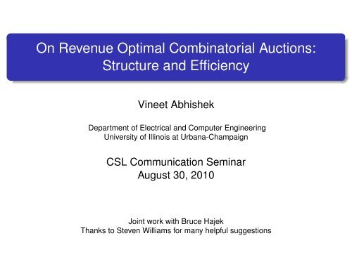
<strong>On</strong> <strong>Revenue</strong> <strong>Optimal</strong> <strong>Combin<strong>at</strong>orial</strong> <strong>Auctions</strong>:<br />
Structure and Efficiency<br />
Vineet Abhishek<br />
Department of Electrical and Computer Engineering<br />
University of Illinois <strong>at</strong> Urbana-Champaign<br />
CSL Communic<strong>at</strong>ion Seminar<br />
August 30, 2010<br />
Joint work with Bruce Hajek<br />
Thanks to Steven Williams for many helpful suggestions
Example - Wireless Spectrum <strong>Auctions</strong><br />
FCC uses auctions to sell rights to use wireless spectrum.<br />
Companies such as AT&T, Verizon, etc, bid for spectrum licenses.<br />
Each bundle of licenses has a value for AT&T, Verizon, etc.<br />
A bundle of licenses might be more valuable than <strong>the</strong> individual<br />
ones.<br />
Objective - maximize FCC’s revenue from spectrum sale.
Wh<strong>at</strong> Makes It Hard?<br />
Priv<strong>at</strong>e values:<br />
The exact value of a bundle of licenses to AT&T is known only to<br />
AT&T.<br />
FCC can only have a rough estim<strong>at</strong>e of it.<br />
Str<strong>at</strong>egic behavior:<br />
AT&T wants to maximize its own profit. Different from FCC’s<br />
objective.<br />
AT&T can misreport its value of a bundle of licenses.
<strong>Combin<strong>at</strong>orial</strong> <strong>Auctions</strong> (CAs)<br />
Provides a common framework for such problems:<br />
Seller - FCC.<br />
Buyers - AT&T, Verizon, etc.<br />
Items - spectrum licenses.<br />
Buyers can compete for any bundle of items.<br />
Alloc<strong>at</strong>ion and payments based on <strong>the</strong> competition.<br />
Design a CA to maximize revenue.
Our Contributions<br />
Most of <strong>the</strong> liter<strong>at</strong>ure on CAs is on efficient auctions.<br />
Maximizing <strong>the</strong> total value gener<strong>at</strong>ed through <strong>the</strong> alloc<strong>at</strong>ion.<br />
Theoretical results on revenue optimal auctions apply only under<br />
simple settings.<br />
Our contributions:<br />
Quantifying how different a revenue optimal auction is from an<br />
efficient auction.<br />
Characterizing revenue optimal auction for a special class of CAs<br />
problems.
Outline<br />
1 Review of revenue optimal auctions<br />
2 Efficiency loss in a revenue optimal auctions<br />
3 <strong>Revenue</strong> maximiz<strong>at</strong>ion for a special class of CAs
Outline<br />
1 Review of revenue optimal auctions<br />
2 Efficiency loss in a revenue optimal auctions<br />
3 <strong>Revenue</strong> maximiz<strong>at</strong>ion for a special class of CAs
Model<br />
N buyers, multiple items.<br />
The bundles desired by <strong>the</strong> buyers are publicly known.<br />
Each desired bundle has <strong>the</strong> same value for a buyer.<br />
A buyer is a winner if he gets any one of his desired bundles.
Model<br />
A Bayesian framework<br />
The value of a buyer n:<br />
A realiz<strong>at</strong>ion of a discrete random variable X n .<br />
X n ∈ {xn 1 , xn 2 , . . . , xn<br />
Kn<br />
}, where 0 ≤ xn 1 < xn 2 < . . . < xn Kn<br />
.<br />
p i n P(X n = x i n), assume p i n > 0.<br />
<strong>On</strong>e-dimensional priv<strong>at</strong>e inform<strong>at</strong>ion:<br />
Beliefs:<br />
The exact realiz<strong>at</strong>ion of X n is known only to buyer n.<br />
X n ’s are independent across <strong>the</strong> buyers.<br />
The probability distributions of X n ’s are common knowledge.
Model<br />
Feasible alloc<strong>at</strong>ions<br />
<strong>Combin<strong>at</strong>orial</strong> constraints restrict <strong>the</strong> set of possible winners, e.g.,<br />
Single item auction - <strong>at</strong> most one buyer can win.<br />
Auction of S identical items - subsets of buyers of size <strong>at</strong> most S.<br />
Each buyer wants a specific bundle of items - subsets of buyers<br />
with disjoint bundles.<br />
A collection of all possible sets of winners.<br />
Assume th<strong>at</strong> A is downward closed:<br />
If A ∈ A and B ⊆ A, <strong>the</strong>n B ∈ A.
The Components of an Auction<br />
.Bid<br />
vector<br />
v<br />
v 1<br />
. .<br />
Alloc<strong>at</strong>ion rule<br />
p(v)<br />
Payment rule<br />
M(v)<br />
Winners<br />
Buyer 1’s<br />
payment py<br />
. . .<br />
v N<br />
Auction<br />
Buyer N’s<br />
payment<br />
π(v) = a probability distribution over A, given v.<br />
π A (v) = P(<strong>the</strong> set of buyers A ∈ A win simultaneously, given v).<br />
The payoff of a buyer = value of <strong>the</strong> alloc<strong>at</strong>ion - payment made.
The High Level Idea<br />
Design a game for revenue maximiz<strong>at</strong>ion:<br />
An auction induces a game of incomplete inform<strong>at</strong>ion among <strong>the</strong><br />
buyers.<br />
Maximize <strong>the</strong> expected revenue <strong>at</strong> its Bayes-Nash equilibrium<br />
(BNE).<br />
Reduce it to a constrained optimiz<strong>at</strong>ion problem:<br />
Truth-telling as a BNE - incentives to be truthful.<br />
This is with no loss of optimality by <strong>the</strong> revel<strong>at</strong>ion principle.<br />
Voluntary particip<strong>at</strong>ion - nonneg<strong>at</strong>ive payoff from particip<strong>at</strong>ion.
The Constraints<br />
First, focus on one buyer:<br />
q(x i ) conditional probability of winning for <strong>the</strong> buyer for bid x i .<br />
m(x i ) expected payment made by <strong>the</strong> buyer for bid x i .<br />
Incentives to be truthful:<br />
q(x i )x i − m(x i ) ≥ q(x k )x i − m(x k ).<br />
Nonneg<strong>at</strong>ive payoff from particip<strong>at</strong>ion:<br />
q(x i )x i − m(x i ) ≥ 0.
Geometric Interpret<strong>at</strong>ion<br />
Let A 0 (0, 0) and A i (q(x i ), m(x i )).<br />
A k must lie above or on <strong>the</strong> line through A i with slope x i .<br />
m(.)<br />
slope = x 3<br />
A 2<br />
slope = x2<br />
A 3 slope = x 1<br />
A 1<br />
A 0 q(x 1 ) q(x 3 ) q(x 2 ) q(.)<br />
x 1 < x 2 < x 3<br />
Non-monotone q(.) : no m(.) can meet <strong>the</strong> constraints!
Geometric Interpret<strong>at</strong>ion<br />
Let A 0 (0, 0) and A i (q(x i ), m(x i )).<br />
A k must lie above or on <strong>the</strong> line through A i with slope x i .<br />
m(.)<br />
A<br />
3<br />
slope = x 3<br />
slope = x 2<br />
A 2 slope = x 1<br />
A 1<br />
A 0 q(x 1 ) q(x 2 ) q(x 3 ) q(.)<br />
x 1 < x 2 < x 3<br />
Monotone q(.) : a suitable m(.) can meet <strong>the</strong> constraints.
Simplifying <strong>the</strong> Constraints<br />
A payment rule s<strong>at</strong>isfying <strong>the</strong> constraints exists if and only if<br />
q(x 1 ) ≤ q(x 2 ) ≤ . . . ≤ q(x K ).<br />
The maximum m(.) for a given q(.) is given by:<br />
m(x i ) =<br />
i∑<br />
k=1<br />
[<br />
]<br />
q(x k ) − q(x k−1 ) x k .<br />
For <strong>the</strong> above m(.), E [m(X)] = E [q(X)w(X)].<br />
w(.) is <strong>the</strong> virtual-valu<strong>at</strong>ion function of <strong>the</strong> buyer.<br />
It suffices to find only an optimal alloc<strong>at</strong>ion rule.
Graphical Construction of Virtual Valu<strong>at</strong>ions<br />
Let X ∈ {x 1 , x 2 , x 3 , x 4 } w.p. {p 1 , p 2 , p 3 , p 4 }.<br />
(0,0) 0)<br />
p 1 p 2 p 3 p 4 (1,0)<br />
−x 1<br />
−x 2<br />
−x 3<br />
−x 4
Graphical Construction of Virtual Valu<strong>at</strong>ions<br />
Let X ∈ {x 1 , x 2 , x 3 , x 4 } w.p. {p 1 , p 2 , p 3 , p 4 }.<br />
(0,0) 0)<br />
p 1 p 2 p 3 p 4 (1,0)<br />
−x 1<br />
−x 2<br />
−x 3<br />
−x 4
Graphical Construction of Virtual Valu<strong>at</strong>ions<br />
Let X ∈ {x 1 , x 2 , x 3 , x 4 } w.p. {p 1 , p 2 , p 3 , p 4 }.<br />
(0,0) 0)<br />
p 1 p 2 p 3 p 4 (1,0)<br />
−x 1<br />
−x 2<br />
−x 3<br />
−x 4
Graphical Construction of Virtual Valu<strong>at</strong>ions<br />
Let X ∈ {x 1 , x 2 , x 3 , x 4 } w.p. {p 1 , p 2 , p 3 , p 4 }.<br />
(0,0) 0)<br />
p 1 p 2 p 3 p 4 (1,0)<br />
−x 1<br />
−x 2<br />
−x 3<br />
−x 4
Graphical Construction of Virtual Valu<strong>at</strong>ions<br />
Let X ∈ {x 1 , x 2 , x 3 , x 4 } w.p. {p 1 , p 2 , p 3 , p 4 }.<br />
(0,0) 0)<br />
p 1 p 2 p 3 p 4 (1,0)<br />
−x 1<br />
−x 2<br />
−x 3<br />
−x 4
Graphical Construction of Virtual Valu<strong>at</strong>ions<br />
Let X ∈ {x 1 , x 2 , x 3 , x 4 } w.p. {p 1 , p 2 , p 3 , p 4 }.<br />
(0,0) 0)<br />
p 1 p 2 p 3 p 4 (1,0)<br />
−x 1<br />
w( x<br />
1 )<br />
−x 2<br />
−x 3<br />
slopes are virtual valu<strong>at</strong>ions, w<br />
−x 4
Graphical Construction of Virtual Valu<strong>at</strong>ions<br />
Let X ∈ {x 1 , x 2 , x 3 , x 4 } w.p. {p 1 , p 2 , p 3 , p 4 }.<br />
(0,0) 0)<br />
p 1 p 2 p 3 p 4 (1,0)<br />
−x 1<br />
w( x<br />
1 )<br />
−x 2<br />
−x 3<br />
slopes are virtual valu<strong>at</strong>ions, w<br />
−x 4
Graphical Construction of Virtual Valu<strong>at</strong>ions<br />
Let X ∈ {x 1 , x 2 , x 3 , x 4 } w.p. {p 1 , p 2 , p 3 , p 4 }.<br />
(0,0) 0)<br />
p 1 p 2 p 3 p 4 (1,0)<br />
−x 1<br />
w( x<br />
1 )<br />
−x 2 w( x<br />
2 )<br />
w( x<br />
3 )<br />
w(x( 4 )<br />
−x 3<br />
slopes are virtual valu<strong>at</strong>ions, w<br />
−x 4
The <strong>Optimal</strong> Auction Problem<br />
Extending <strong>the</strong> analysis to N buyers:<br />
[ ∑N<br />
]<br />
Under truth-telling, <strong>the</strong> expected revenue = E<br />
n=1 M n(X) ,<br />
where <strong>the</strong> random vector X {X 1 , X 2 , . . . , X N }.<br />
The <strong>Optimal</strong> Auction Problem (OAP)<br />
maximize<br />
π,M<br />
[ N<br />
]<br />
∑<br />
E M n (X) ,<br />
n=1<br />
subject to: truth-telling and voluntary particip<strong>at</strong>ion.
Simplifying OAP<br />
<strong>Revenue</strong>(π) maximum revenue to <strong>the</strong> seller for a given π,<br />
[ N<br />
]<br />
∑<br />
= E q n (X n )w n (X n ) (from single buyer analysis),<br />
n=1<br />
[ ∑<br />
= E π A (X) ( ∑<br />
w n (X n ) )] (by rel<strong>at</strong>ing q n ’s to π).<br />
A∈A<br />
n∈A
Simplifying OAP<br />
<strong>Revenue</strong>(π) maximum revenue to <strong>the</strong> seller for a given π,<br />
[ N<br />
]<br />
∑<br />
= E q n (X n )w n (X n ) (from single buyer analysis),<br />
n=1<br />
[ ∑<br />
= E π A (X) ( ∑<br />
w n (X n ) )] (by rel<strong>at</strong>ing q n ’s to π).<br />
A∈A<br />
n∈A<br />
Suggests alloc<strong>at</strong>ing from argmax<br />
A∈A<br />
[ ∑<br />
w n (v n ) ] , for a bid vector v.<br />
n∈A<br />
Works if w n (x 1 n ) ≤ w n (x 2 n ) ≤ . . . ≤ w n (x Kn<br />
n ).<br />
O<strong>the</strong>rwise, <strong>the</strong> resulting q n ’s need not be monotone.
Simplifying OAP<br />
Replace w n ’s by monotone virtual valu<strong>at</strong>ions (MVVs), w n .<br />
p 1 p 2 p 3 p 4 (1,0)<br />
(0,0)<br />
w( x<br />
1 )<br />
−x 1<br />
w( x<br />
2 )<br />
−x 2 _<br />
w( x<br />
1 )<br />
_<br />
4<br />
4<br />
_<br />
w ( x ) = w(<br />
x )<br />
w( x<br />
2 )<br />
_<br />
3<br />
3<br />
w ( x ) = w(<br />
x )<br />
−x 3<br />
slopes are virtual valu<strong>at</strong>ions, w _<br />
slopes are monotone virtual valu<strong>at</strong>ions, w<br />
−x 4
The Maximum Weight Algorithm (MWA)<br />
Given a bid vector v:<br />
1 Compute w n (v n ) for each n.<br />
2 π(v) = a probability distribution on argmax<br />
A∈A<br />
[ ∑<br />
w n (v n ) ] .<br />
n∈A<br />
3 Collect payments given by:<br />
M n (v) =<br />
∑ [<br />
Qn (xn, i v −n ) − Q n (xn i−1 , v −n ) ] xn,<br />
i<br />
i:xn≤v i n<br />
where Q n (v) = P(buyer n wins, given <strong>the</strong> bid vector v).
Reserve Prices<br />
No buyer n with w n (v n ) < 0 is a winner under MWA.<br />
Follows since A is downward-closed and ∅ ∈ A.<br />
Equivalently, <strong>the</strong> seller sets a reserve price for each buyer n.<br />
Follows since MVVs are nondecresing functions.<br />
The reserve price for buyer n = minimum v n such th<strong>at</strong> w n (v n ) > 0.
Outline<br />
1 Review of revenue optimal auctions<br />
2 Efficiency loss in a revenue optimal auctions<br />
3 <strong>Revenue</strong> maximiz<strong>at</strong>ion for a special class of CAs
Efficient <strong>Auctions</strong><br />
An alloc<strong>at</strong>ion of items among buyers gener<strong>at</strong>es value for <strong>the</strong><br />
items.<br />
The realized social welfare (RSW) = total value gener<strong>at</strong>ed<br />
through <strong>the</strong> alloc<strong>at</strong>ion of items.<br />
An efficient auction maximizes <strong>the</strong> realized social welfare.<br />
For a bid vector v, an efficient alloc<strong>at</strong>ion is a probability<br />
( ∑ )<br />
distribution on argmax v n .<br />
A∈A<br />
n∈A
Some Questions<br />
How different is a revenue optimal auction from an efficient<br />
auction?<br />
Wh<strong>at</strong> causes <strong>the</strong>se differences?<br />
How to quantify this difference?<br />
Wh<strong>at</strong> are <strong>the</strong> underlying parameters?<br />
We answer <strong>the</strong>se.
<strong>Revenue</strong> vs Efficiency - Example 1<br />
The role of reserve prices:<br />
Buyer 1 Buyer 2<br />
1/3 2/3 1/3 2/3<br />
$1 $2 $1 $2
<strong>Revenue</strong> vs Efficiency - Example 1<br />
The role of reserve prices:<br />
Buyer 1 Buyer 2<br />
1/3 2/3 1/3 2/3<br />
$1 $2 $1 $2<br />
Efficient auction<br />
Sell to <strong>the</strong> highest bidder <strong>at</strong> <strong>the</strong> second<br />
highest price.<br />
<strong>Revenue</strong> = 2*(2/3) 2 + 1 ‐ (2/3) 2 @ $1.45.<br />
MSW = 2*( 1 ‐ (1/3) 2 ) + (1/3) 2 @ $1.89.
<strong>Revenue</strong> vs Efficiency - Example 1<br />
The role of reserve prices:<br />
Buyer 1 Buyer 2<br />
1/3 2/3 1/3 2/3<br />
$1 $2 $1 $2<br />
Efficient auction<br />
<strong>Revenue</strong> optimal auction<br />
Sell to <strong>the</strong> highest bidder <strong>at</strong> <strong>the</strong> second<br />
Set reserve price = $2, sell to anyone<br />
highest price.<br />
who bids $2.<br />
<strong>Revenue</strong> = 2*(2/3) 2 + 1 ‐ (2/3) 2 @ $1.45. <strong>Revenue</strong> = 2*( 1 ‐ (1/3) 2 ) @ $1.77.<br />
MSW = 2*( 1 ‐ (1/3) 2 ) + (1/3) 2 @ $1.89. RSW = 2*( 1 ‐ (1/3) 2 ) @ $1.77.
<strong>Revenue</strong> vs Efficiency - Example 2<br />
The buyer with <strong>the</strong> highest valu<strong>at</strong>ion need not win:<br />
Buyer 1 Buyer 2<br />
1/2 1/2 1/2 1/2<br />
$5 $10 $1 $2
<strong>Revenue</strong> vs Efficiency - Example 2<br />
The buyer with <strong>the</strong> highest valu<strong>at</strong>ion need not win:<br />
Buyer 1 Buyer 2<br />
1/2 1/2 1/2 1/2<br />
$5 $10 $1 $2<br />
Efficient auction<br />
Always sell to buyer 1.<br />
Price charged can be <strong>at</strong> most $5.<br />
MSW = (10 + 5)*0.55 = $7.5.
<strong>Revenue</strong> vs Efficiency - Example 2<br />
The buyer with <strong>the</strong> highest valu<strong>at</strong>ion need not win:<br />
Buyer 1 Buyer 2<br />
1/2 1/2 1/2 1/2<br />
$5 $10 $1 $2<br />
Efficient auction<br />
<strong>Revenue</strong> optimal auction<br />
Always sell to buyer 1.<br />
Sell to buyer 1 if v 1 = $10 <strong>at</strong> $10, else sell<br />
to buyer 2 <strong>at</strong> $1.<br />
Price charged can be <strong>at</strong> most $5. <strong>Revenue</strong> = (10 + 1)*0.5 = $5.5.<br />
MSW = (10 + 5)*0.55 = $7.5. RSW = (10 + 0.5*(2 05*(2+ 1))*0.5 = $5.75.
<strong>Revenue</strong> vs Efficiency - Example 3<br />
Efficiency loss in multiple items case:<br />
A Buyer 1<br />
B Buyer 2 C Buyer 3<br />
D<br />
1/2 1/2<br />
1/2 1/2 1/2 1/2<br />
$1 $1.6 $1 $1.6 $1 $1.6<br />
Buyers 1 & 2, or Buyer 2 & 3 cannot win simultaneously.
<strong>Revenue</strong> vs Efficiency - Example 3<br />
Efficiency loss in multiple items case:<br />
A Buyer 1<br />
B Buyer 2 C Buyer 3<br />
D<br />
1/2 1/2<br />
1/2 1/2 1/2 1/2<br />
$1 $1.6 $1 $1.6 $1 $1.6<br />
Buyers 1 & 2, or Buyer 2 & 3 cannot win simultaneously.<br />
w n ($1) = $0.4, w n ($1.6) = $1.6.<br />
For <strong>the</strong> bid vector ($1, $1.6, $1):<br />
Efficient auction alloc<strong>at</strong>es to buyers 1 and 3.<br />
<strong>Revenue</strong> optimal auction alloc<strong>at</strong>es to buyer 2.
Quantifying Efficiency Loss<br />
RSW by an alloc<strong>at</strong>ion rule π:<br />
[ ∑<br />
RSW(π, X; A) = E π A (X) ( ∑ ) ]<br />
X n .<br />
A∈A n∈A<br />
Maximum social welfare (MSW) (by an efficient alloc<strong>at</strong>ion):<br />
[<br />
( ∑ ) ]<br />
MSW(X; A) = E X n .<br />
max<br />
A∈A<br />
n∈A<br />
The RSW by an optimal alloc<strong>at</strong>ion ≤ MSW.
Quantifying Efficiency Loss<br />
For an optimal alloc<strong>at</strong>ion rule π o , define <strong>the</strong> efficiency loss r<strong>at</strong>io<br />
(ELR) as:<br />
ELR(π o , X; A) MSW(X; A) − RSW(πo , X; A)<br />
MSW(X; A)<br />
The Worst Case ELR Problem<br />
maximize ELR(π o , X; A),<br />
X<br />
subject to: K n ≤ K for all n, and (max n xn Kn )/(min n xn 1 ) ≤ r.<br />
Denote <strong>the</strong> worst case ELR by η(r, K ; A) for r ≥ 1 and K ≥ 1.
Worst Case ELR Comput<strong>at</strong>ion - Example<br />
Buyer 1<br />
1‐p p 0 < L < H<br />
r = H/L<br />
L H
Worst Case ELR Comput<strong>at</strong>ion - Example<br />
Buyer 1<br />
1‐p p 0 < L < H<br />
r = H/L<br />
L H<br />
If pr < 1, <strong>the</strong>n w(L) > 0. The optimal alloc<strong>at</strong>ions is efficient.<br />
If pr ≥ 1, <strong>the</strong>n w(L) ≤ 0. The buyer wins only if he bids H.
Worst Case ELR Comput<strong>at</strong>ion - Example<br />
Buyer 1<br />
1‐p p 0 < L < H<br />
r = H/L<br />
L H<br />
If pr < 1, <strong>the</strong>n w(L) > 0. The optimal alloc<strong>at</strong>ions is efficient.<br />
If pr ≥ 1, <strong>the</strong>n w(L) ≤ 0. The buyer wins only if he bids H.<br />
For pr ≥ 1, <strong>the</strong> RSW = pH, while <strong>the</strong> MSW = pH + (1 − p)L.<br />
ELR = (1 − p)/(pr + 1 − p).
Worst Case ELR Comput<strong>at</strong>ion - Example<br />
Buyer 1<br />
1‐p p 0 < L < H<br />
r = H/L<br />
L H<br />
If pr < 1, <strong>the</strong>n w(L) > 0. The optimal alloc<strong>at</strong>ions is efficient.<br />
If pr ≥ 1, <strong>the</strong>n w(L) ≤ 0. The buyer wins only if he bids H.<br />
For pr ≥ 1, <strong>the</strong> RSW = pH, while <strong>the</strong> MSW = pH + (1 − p)L.<br />
ELR = (1 − p)/(pr + 1 − p).<br />
ELR is maximized by setting p = 1/r.<br />
Hence, η = (r − 1)/(2r − 1).
ELR Bound - Binary Valued Buyers<br />
Proposition (Abhishek and Hajek 2010)<br />
Suppose A is downward closed. Given any r > 1, <strong>the</strong> worst case ELR<br />
for binary valued buyers, denoted by η(r, 2; A), s<strong>at</strong>isfies:<br />
η(r, 2; A) ≤ (r − 1)/(2r − 1).<br />
The worst case ELR for N buyers (not necessarily identically<br />
distributed) is no worse than it is for single buyer!<br />
Holds for arbitrary downward closed A.<br />
The worst case ELR ≤ 1/2 uniformly over all r.
ELR Bound - Single Item <strong>Auctions</strong> with i.i.d. Buyers<br />
Moving beyond binary valu<strong>at</strong>ions but restricting to single item.<br />
Reduction to a rel<strong>at</strong>ively simpler optimiz<strong>at</strong>ion problem involving<br />
only <strong>the</strong> common probability vector of <strong>the</strong> buyers.<br />
Lower and upper bounds (asymptotically tight as K → ∞) on <strong>the</strong><br />
worst case ELR.<br />
The worst case ELR → 0 as N → ∞ <strong>at</strong> <strong>the</strong> r<strong>at</strong>e O ( (1 − 1/r) N) .<br />
The worst case ELR → 1 as K → ∞ and r → ∞.
Outline<br />
1 Review of revenue optimal auctions<br />
2 Efficiency loss in a revenue optimal auctions<br />
3 <strong>Revenue</strong> maximiz<strong>at</strong>ion for a special class of CAs
Limit<strong>at</strong>ions of General CAs<br />
Implement<strong>at</strong>ion complexity:<br />
Alloc<strong>at</strong>ion problem is NP-hard in general.<br />
Large communic<strong>at</strong>ion overhead.<br />
Current st<strong>at</strong>e of <strong>the</strong> art:<br />
General results on revenue maximiz<strong>at</strong>ion known only for<br />
one-dimensional problems.<br />
Joint problem of tractability and characteriz<strong>at</strong>ion.
Single-Minded Buyers<br />
A rel<strong>at</strong>ively more tractable class of CAs.<br />
Each buyer is interested only in a specific bundle.<br />
Both <strong>the</strong> bundle and its value are known only to <strong>the</strong> buyer.<br />
Any bundle of items not containing his desired bundle has zero<br />
value for him.
Why Study Single-Minded Buyers Model?<br />
Key is to understand and handle complementarity.<br />
A bundle as a whole can be more valuable than <strong>the</strong> sum of values<br />
of its parts.<br />
Single-minded buyers - an extreme case of complementarity.<br />
Problem is still nontrivial (two dimensional):<br />
A buyer can misreport both his bundle and its value.<br />
No general result on revenue maximiz<strong>at</strong>ion is known even for<br />
this extreme case.<br />
Some real examples where buyers are single minded.
Extending <strong>the</strong> Model to Single-Minded Buyers<br />
The type of a buyer n = (bundle, value).<br />
Bundles of a buyer n - a realiz<strong>at</strong>ion of a random set B n .<br />
Value of a buyer n - a realiz<strong>at</strong>ion of a discrete random variable X n .<br />
Two-dimensional priv<strong>at</strong>e inform<strong>at</strong>ion:<br />
The exact realiz<strong>at</strong>ion of (B n , X n ) is known only to buyer n.<br />
Beliefs:<br />
(B n , X n )’s are independent across <strong>the</strong> buyers.<br />
The joint probability distribution of (B n , X n ) is common knowledge.
Extending <strong>the</strong> Model to Single-Minded Buyers<br />
The bid vector (b, v) = reported vector of (bundles, values).<br />
The collection of all possible sets of winners, A(b), depends on b.<br />
A ∈ A(b) if <strong>the</strong> reported bundles of buyers in set A are disjoint.<br />
The alloc<strong>at</strong>ion rule π and payments M depend jointly on (b, v).<br />
The virtual-valu<strong>at</strong>ion function, w n (b n , v n ), is now constructed from<br />
<strong>the</strong> condition random variable (X n |B n = b n ).
A Candid<strong>at</strong>e for <strong>the</strong> <strong>Revenue</strong> <strong>Optimal</strong> Auction<br />
Given a bid vector (b, v):<br />
Construct a conflict graph G b :<br />
A node n for each buyer n.<br />
An edge e n,m if b n ∩ b m ≠ ∅.<br />
Assign a weight w n (b n , v n ) to node n.<br />
Set of winners = maximum weight independent set of G b .<br />
Winner’s payment = <strong>the</strong> minimum value he needs to report to win.
Does It Work?<br />
Buyer 1 Buyer 2<br />
1<br />
1/2 1/2<br />
Bundle {A}<br />
Bundle {A} Bundle {A,B}<br />
1<br />
1/2 1/2 9/10 1/10<br />
$1 $2 $4 $2 $4<br />
__ __ __ __ __<br />
W = $1 W = $0 W = $4 W = $16/9 W = $4
Does It Work?<br />
Buyer 1 Buyer 2<br />
1<br />
1/2 1/2<br />
Bundle {A}<br />
Bundle {A} Bundle {A,B}<br />
1<br />
1/2 1/2 9/10 1/10<br />
$1 $2 $4 $2 $4<br />
__ __ __ __ __<br />
W = $1 W = $0 W = $4 W = $16/9 W = $4<br />
For <strong>the</strong> bid ({A}, $4), buyer 2 gets <strong>the</strong> bundle {A} for $4.<br />
For <strong>the</strong> bid ({A, B}, $4), buyer 2 gets <strong>the</strong> bundle {A, B} for $2.
Does It Work?<br />
Buyer 1 Buyer 2<br />
1<br />
1/2 1/2<br />
Bundle {A}<br />
Bundle {A} Bundle {A,B}<br />
1<br />
1/2 1/2 9/10 1/10<br />
$1 $2 $4 $2 $4<br />
__ __ __ __ __<br />
W = $1 W = $0 W = $4 W = $16/9 W = $4<br />
For <strong>the</strong> bid ({A}, $4), buyer 2 gets <strong>the</strong> bundle {A} for $4.<br />
For <strong>the</strong> bid ({A, B}, $4), buyer 2 gets <strong>the</strong> bundle {A, B} for $2.<br />
Thus, buyer 2 will misreport type ({A}, $4) as ({A, B}, $4).<br />
A counter example!
Wh<strong>at</strong> Went Wrong?<br />
An arbitrary joint distribution of (bundles, values) causes<br />
problems.<br />
If w n (b n , v n ) is increasing in b n , buyer n will bid for a larger bundle.<br />
A possible fix - assume B n and X n to be independent.<br />
Works well m<strong>at</strong>hem<strong>at</strong>ically, but an unreasonable assumption.<br />
A reasonable assumption - <strong>the</strong> value of <strong>the</strong> larger of two bundles<br />
is likely to be higher.<br />
Wh<strong>at</strong> is <strong>the</strong> precise condition for optimality?
The Sufficient Condition<br />
Hazard r<strong>at</strong>e order<br />
Let Z 1 , Z 2 be nonneg<strong>at</strong>ive random variables. Z 1 ≤ h Z 2 , if<br />
Prob(Z 1 > z|Z 1 > ẑ) ≤ Prob(Z 2 > z|Z 2 > ẑ) for all z ≥ ẑ.<br />
Stronger than <strong>the</strong> first order stochastic dominance.<br />
The sufficient condition<br />
Let s ⊆ t be two bundles. Then (X n |B n = s) ≤ h (X n |B n = t).<br />
The larger bundle is likely to have higher value.<br />
The condition is intuitive for single-minded buyers.
Main Result<br />
Proposition (Abhishek and Hajek 2010)<br />
If <strong>the</strong> conditional distribution of X n given B n = s is nondecreasing in s,<br />
in <strong>the</strong> hazard r<strong>at</strong>e ordering on probability distributions, <strong>the</strong>n<br />
1 w n (s, v n ) ≥ w n (t, v n ) if s ⊆ t,<br />
2 <strong>the</strong> candid<strong>at</strong>e auction s<strong>at</strong>isfies truth-telling and voluntary<br />
particip<strong>at</strong>ion constraints,<br />
3 <strong>the</strong> candid<strong>at</strong>e auction is revenue optimal.
Concluding Remarks<br />
A revenue optimal auction can be very different from an<br />
efficient auction.<br />
Characterizing revenue optimal CA in full generality - an open<br />
problem.<br />
A possible direction - reducing str<strong>at</strong>egy space and imposing some<br />
structure on priv<strong>at</strong>e inform<strong>at</strong>ion.<br />
The single-minded buyers model - an initial step towards solving<br />
<strong>the</strong> general CA problems.