N-Body Simulation
N-Body Simulation
N-Body Simulation

You also want an ePaper? Increase the reach of your titles
YUMPU automatically turns print PDFs into web optimized ePapers that Google loves.
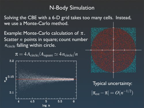
N-<strong>Body</strong> <strong>Simulation</strong><br />
Solving the CBE with a 6-D grid takes too many cells. Instead,<br />
we use a Monte-Carlo method.<br />
Example: Monte-Carlo calculation of π .<br />
Scatter<br />
n circle<br />
n<br />
points in square; count number<br />
falling within circle.<br />
π = 4A circle /A square ≃ 4n circle /n<br />
Typical uncertainty:<br />
|π est − π| = O(n −1/2 )
Representing the Distribution Function<br />
Replace smooth distribution with bodies:<br />
f (⃗r,⃗v) → {(m i ,⃗r i ,⃗v i ) | i = 1,...,N}<br />
f (⃗r,⃗v) ≃<br />
This requires that for any phase-space volume V,<br />
Z<br />
〈 〉<br />
d⃗rd⃗v f (⃗r,⃗v) = ∑ m (⃗ri ,⃗v i )∈V i<br />
E.g., select (⃗r i ,⃗v i ) with probability proportional to f (⃗r i ,⃗v i ), and<br />
assign all bodies equal mass:<br />
V<br />
N<br />
∑ m i δ 3 (⃗r −⃗r i )δ 3 (⃗v −⃗v i )<br />
i=1<br />
m i = 1 N<br />
Z<br />
d⃗rd⃗v f (⃗r,⃗v)
Advancing Time<br />
Move bodies along phase flow (method of characteristics):<br />
Estimate potential from N-body representation:<br />
This will yield the usual N-body equation for point masses. But<br />
singular potentials are awkward, so we smooth the density field:<br />
δ 3 (⃗r −⃗r i ) → 3<br />
4π<br />
ε 2<br />
(|⃗r −⃗r i | 2 + ε 2 ) 5/2<br />
This substitution yields the following equations of motion:<br />
d⃗r i<br />
dt =⃗v i<br />
(˙ ⃗r i , ˙ ⃗v i ) = (⃗v i ,−(∇Φ) i )<br />
∇ 2 Φ ∣ ∣<br />
⃗r<br />
= 4πG<br />
d⃗v i<br />
dt = N<br />
∑<br />
j≠i<br />
N<br />
∑ m i δ 3 (⃗r −⃗r i )<br />
i=1<br />
Gm j (⃗r j −⃗r i )<br />
(|⃗r j −⃗r i | 2 + ε 2 ) 3/2<br />
Plummer (1911)<br />
smoothing<br />
Aarseth (1963)
Comments<br />
1. N-body models relax at roughly the same rate as real stellar<br />
systems with the same<br />
N<br />
; the relaxation time is<br />
t r ≃<br />
N<br />
8ln(R /ε) t c<br />
2. Sampling proportional to f (⃗r i ,⃗v i ) is the simplest option, but<br />
not the only one; other weighting schemes are also possible.<br />
E.g., use different masses when sampling f s (⃗r,⃗v) and f d (⃗r,⃗v) , or<br />
make m i depend on f (⃗r i ,⃗v i ) . But note effect on relaxation time!<br />
3. Plummer smoothing is just one of many possibilities, and may<br />
not be optimal; one alternative with less of a “tail” is<br />
δ 3 (⃗r −⃗r i ) → 15<br />
ε 4<br />
8π (|⃗r −⃗r i | 2 + ε 2 ) 7/2 Dehnen (2001)
Force Calculation: Direct Summation<br />
Simplest method: sum over all other bodies.<br />
⃗a i =<br />
N<br />
∑<br />
j≠i<br />
Gm j (⃗r j −⃗r i )<br />
(|⃗r j −⃗r i | 2 + ε 2 ) 3/2<br />
Advantages: robust, accurate, completely general.<br />
Disadvantage: computational cost per body is O(N) ;<br />
need O(N 2 ) operations to compute forces on all bodies.<br />
However, direct summation is a good fit with<br />
1. Individual timesteps (see Sverre’s lectures)<br />
2. Specialized hardware (see Simon’s lectures)
Tree Codes<br />
Long-range gravitational field dominated<br />
by monopole term:<br />
φ ≃ − Gm<br />
r + O(r−3 )<br />
Divide system into hierarchy (i.e.“tree”)<br />
of compact cells:<br />
Saul Steinberg, “A view of the World from 9 th Avenue, 1976.<br />
Barnes & Hut (1986)<br />
Replace sum over N bodies with sum<br />
over N c ≃ O(logN) cells; cost to find<br />
forces on all bodies is O(N logN) .<br />
N<br />
∑<br />
i<br />
→<br />
N c<br />
∑<br />
c
Tree Codes Continued<br />
1. To compute potential at ⃗r due to a cell c :<br />
a) if c is “too close” to ⃗r , sum the potentials of its sub-cells;<br />
b) otherwise, approximate the potential as −Gm c /|⃗r −⃗r c | .<br />
2. “too close” can be defined in various ways; e.g.:<br />
cell’s center<br />
of mass<br />
a) geometrically: |⃗r −⃗r c | < l c /θ (BH86) or < l c /θ + δ c (B95),<br />
b) dynamically: |⃗r −⃗r c | 4 < GM c l 2 c/α|⃗a| (GADGET-2: Springel 2005).<br />
3. Different tree structures give roughly equivalent results:<br />
a) oct-trees: 1 cube → 8 cubes (Barnes & Hut 1986),<br />
b) kd trees: divide at median along x,y,z (Dikaiakos & Stadel 1996),<br />
c) particle trees: group nearest neighbors (Appel 1985, Press 1986).<br />
4. Higher moments improve accuracy:<br />
a) quadrupole potential term:<br />
1<br />
2Gδ⃗r · Q c · δ⃗r /δr 5 (Hernquist 1987),<br />
b) source/sink symmet. momentum cons., O(N) (Dehnen 2000).
Self-Consistent Field Method<br />
Represent potential and density as sums:<br />
Φ(⃗r) = ∑<br />
k<br />
A k Φ k (⃗r),<br />
ρ(⃗r) = ∑<br />
k<br />
A k ρ k (⃗r)<br />
where are coefficients and the basis functions and are<br />
A k<br />
bi-orthogonal and satisfy the PE:<br />
I k δ k k<br />
′ =<br />
Z<br />
d⃗r ρ k (⃗r)[Φ k ′(⃗r)] ∗ ,<br />
The coefficients are computed using overlap integrals:<br />
A k = 1 Z<br />
d⃗r ρ(⃗r)[Φ k (⃗r)] ∗ = 1 ∑m i [Φ k (⃗r i )] ∗<br />
I k I k<br />
Φ k<br />
∇ 2 Φ k = 4πGρ k<br />
The cost of calculating forces on all bodies is just O(N) .<br />
ρ k<br />
With the right basis set, SCFM yields good forces for spheroidal<br />
systems with only a few terms (Hernquist & Ostriker 1992).
Time Step Algorithms<br />
The underlying symmetry of the N-body equation of motion<br />
becomes evident in Hamiltonian formulation:<br />
d⃗r<br />
dt = ∂H<br />
∂⃗p ,<br />
d⃗p<br />
dt = −∂H ∂⃗r<br />
This symmetry has important consequences:<br />
1. dynamical evolution conserves phase space volume<br />
2. Hamiltonian systems have no attractors<br />
3. dynamical evolution is reversible.<br />
Hamiltonian systems are not structurally stable; most<br />
integrators will not preserve these properties.<br />
An integration algorithm with Hamiltonian symmetry is<br />
desirable; such an integrator is known as symplectic.
Leapfrog Integrator<br />
This very simple integrator explicitly preserves the symmetry<br />
of the Hamiltonian equations of motion:<br />
⃗r [k+1]<br />
i<br />
⃗v [k+3/2]<br />
i<br />
⃗v [k+1/2]<br />
i<br />
=⃗r [k]<br />
i<br />
+∆t⃗v [k+1/2]<br />
i<br />
=⃗v [k+1/2]<br />
i +∆t⃗a i (⃗r [k+1] )<br />
In addition, it is accurate to second order, meaning that the error<br />
is<br />
O(∆t 3 )<br />
per step, and requires very little storage.<br />
A drawback of the leapfrog is that velocities are a half-step out<br />
of sync with positions; this can be avoided as follows:<br />
⃗r [k+1]<br />
i<br />
⃗v [k+1]<br />
i<br />
=⃗v [k]<br />
i<br />
=⃗r [k]<br />
i<br />
=⃗v [k+1/2]<br />
i<br />
+ ∆t<br />
2 ⃗a i(⃗r [k] )<br />
+∆t⃗v [k+1/2]<br />
i<br />
+ ∆t<br />
2 ⃗a i(⃗r [k+1] )<br />
This formulation introduces a one-time error of<br />
otherwise equivalent to the standard leapfrog.<br />
O(∆t 2 )<br />
but is
Individual Time Steps?<br />
Leapfrog becomes inaccurate if ∆t is not constant<br />
and identical for all bodies. This seems inefficient.<br />
However, the symplectic properties of the leapfrog<br />
give it much more stability than most integrators.<br />
Algorithms in which ∆t is determined by current<br />
conditions are not reversible. Symmetrizing the<br />
time step between endpoints t and t + ∆t works<br />
but imposes a significant overhead (Hut et al. 1995).<br />
A 4 th order symplectic scheme allowing individual<br />
and adaptive time-steps is now available (Farr &<br />
Bertschinger 2007).<br />
Springel (2005)
Errors and Relaxation<br />
N-body simulations diverge from exact<br />
solutions of CBE and PE for several reasons:<br />
1. Roundoff errors.<br />
2. Truncation in time stepping.<br />
3. Force calculation approximations.<br />
4. Density field smoothing.<br />
5. Relaxation due to finite N.<br />
“An Introduction to Error Analysis”, John R. Taylor<br />
In theory, these effects can all be controlled — at a price. Error<br />
#1 is seldom an issue, while errors #2 and #3 are easily limited.<br />
Smoothing and relaxation are harder to balance; high resolution<br />
demands shorter timesteps and more bodies.<br />
Finally, all N-body systems with N > 2 are potentially chaotic,<br />
while the role of chaos in real galaxies is unclear.
Parameter Choices<br />
The number of bodies<br />
N<br />
is the key parameter:<br />
— 2-body relaxation time: t r ≃ Nt c /8ln(R /ε)<br />
— Monte-Carlo errors: O(N −1/2 )<br />
Maximum duration of simulation must be . t ≪ t r<br />
Typical errors in acceleration should be |δa/a| N −1/2 .<br />
Global energy should be conserved to |δE/E| N −1/2 .<br />
Smoothing length is typically R N −1/2 < ε < R N −1/3 .<br />
Leapfrog time-step should be ∆t 0.03t min ≃ 0.09(Gρ max ) −1/2 .<br />
WARNING: these rules are not definitive. Tests with different<br />
parameter values are useful; a skeptical attitude is advised!
Introduction to Smoothed Particle Hydrodynamics<br />
Fluid equations in conservation form:<br />
mass:<br />
momentum:<br />
∂ρ<br />
∂t + ∇ · (ρ⃗v) = 0<br />
∂⃗v<br />
∂t + (⃗v · ∇)⃗v = −∇Φ + 1 ρ ∇P<br />
energy or<br />
entropy:<br />
<br />
<br />
<br />
∂u<br />
∂t + (⃗v · ∇)u = −P ∇ ·⃗v + ˙u<br />
ρ<br />
∂a<br />
∂t + (⃗v · ∇)a = (γ − 1)ρ1−γ ˙u<br />
Equation of state (ideal gas):<br />
P = (γ − 1)ρu<br />
P = a(S)ρ γ
ρ(⃗r),⃗v(⃗r), u(⃗r), a(⃗r) → {(m i ,⃗r i ,⃗v i , u i , a i ) | i = 1,...,N}<br />
d⃗r i<br />
dt =⃗v i<br />
du i<br />
dt = (<br />
− P ρ ∇ ·⃗v )<br />
i<br />
SPH Formalism<br />
Particle representation (c.f. N-body):<br />
Density estimate uses smoothing kernel W(⃗x,h) with scale h :<br />
N<br />
ρ(⃗r) ≃ ∑m i W(⃗r −⃗r i ,h)<br />
i<br />
R<br />
where d⃗xW(⃗x,h) = 1 ; estimates of gradients become sums<br />
involving gradients of W(⃗x,h) .<br />
Dynamical equations:<br />
d⃗v i<br />
dt = (−∇Φ) i + (<br />
− 1 ρ ∇P )<br />
+ ˙u i + ˙u visc<br />
i<br />
da i<br />
dt<br />
i<br />
+⃗a visc<br />
i<br />
= (γ − 1)ρ1−γ i<br />
( ˙u i + ˙u visc<br />
i )
Comments<br />
1. The smoothing kernel W(⃗x,h) has compact support, so only<br />
nearby bodies are included in the sums. Most SPH codes adapt<br />
the smoothing length h to the local particle density.<br />
2. Adaptive timesteps are generally necessary to satisfy the<br />
Courant condition; most SPH integrators are not symplectic.<br />
3. Artificial viscosity is required to keep particles from streaming<br />
through shocks. The best formulation is not entirely clear.<br />
4. SPH is often criticized as a poor approximation to proper gas<br />
dynamics. However, the ISM is much more complex than an ideal<br />
gas. In the context of galaxy-scale simulations, momentum and<br />
energy conservation may be all we can expect of a code.