Polarization and Polarization Controllers - NTNU

Polarization and Polarization Controllers
Vegard L. Tuft (vegard.tuft@iet.ntnu.no)
Version: September 14, 2007
Abstract: This document is an introduction to polarization controllers and their
applications in fiber optical communication systems. Using Jones representation, it
provides a mathematical overview of polarization before describing the concept of wave
plates and how to cascade wave plates to form a polarization controller. The principles of
operation of two different controllers are described: Lefevre’s three-loop rotating wave
plate device and General Photonics’ PolaRite rotating variable-phase controller.
1 Introduction – Why Polarization Controllers?
Figure 1 illustrates a situation in which light from a laser is guided by an optical fiber and enters an
optical component. In many cases the performance of the component depends on the polarization of the
light. Wavelength multiplexers, wavelength converters, modulators, amplifiers, interferometers and
some receivers are examples of devices that are polarization sensitive. An irregular fiber core as well as
thermal and mechanical stress causes the light to change its state of polarization (SOP) as it propagates
in standard single-mode fibers - this in a random and time-varying way due to ever-changing
environmental conditions. The time-varying polarization states can also cause random pulse spreading
and signal distortions as the signal propagates through the fiber, a phenomenon called polarizationmode
dispersion (PMD). Therefore, in order to overcome these challenges, we need a device that can,
in a controllable and predictable way, change the SOP into the desired state at the fiber output.
Laser
Fiber optic
transmission line
Polarization controller
Figure 1: Basic transmission system with polarization controller.
Optical
component
This document first summarizes the mathematical foundation for describing and analyzing such a
device, by using Jones representation of the light and the Poincaré sphere. Then, we analyze cascaded
wave retarders and the principle of operation of polarization controllers. The retarders are often refered
to as wave plates. Furthermore, two fiber optic implementations using rotating wave retarders are
presented. Finally, we will have a brief look at three typical applications of polarization controllers in
optical communication systems: polarization optimization, PMD compensation, and de-multiplexing of
polarization multiplexed signals.
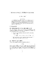
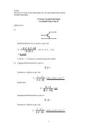
2 Mathematical Description of Polarized Light
2.1 The Polarization Ellipse
We will in the following consider a monochromatic optical field of frequency ν and wavelength λ
traveling in the z direction through a standard step-index single mode fiber. In the scalar
approximation, which is valid when the difference between core and cladding refractive index is small,
we can write the field as a transversal mode Ψ(x,y) in the (x,y) plane perpendicular to and independent
of the propagation direction:
( E xˆ
+ E ˆ ) Ψ( x y)
E = y , (1)
x y ,

where
{ }
{ }
i
( )
( τ + 1
τ + δ
)
1 = R a1e
i
( )
( τ + δ 2
τ + δ = R a e
)
1 cos δ
E = a
(2a)
x
E = a2 cos 2 2 . (2b)
y
τ = ωt-βz, where ω = 2πν is the angular frequency and β = 2π/λ is the propagation constant of the mode.
By eliminating τ between E x and E y into (2a-b) we obtain the equation of the polarization ellipse [1]
⎛ E
⎜
⎝ a
x
1
⎞
⎟
⎠
2
⎛ E
+ ⎜
⎝ a
y
2
⎞
⎟
⎠
2
E E
x y
− 2 cosδ
= sin
a a
1
2
2
δ . (3)
δ = δ 2 - δ 1 is the phase difference between the x and y components of the electrical field. This ellipse is
in general rotated through an angle ψ, as illustrated in Fig. 2, due to the cross-term E x ·E y :
2a1a
cosδ
tan 2ψ =
. (4)
a − a
2
2
1
2
2
y
E
2a 2
ψ
θ
x
2a 1
Figure 2: The polarization ellipse and describing parameters.
For any given position z, the tip of the electrical field vector E follows an elliptical path in the (x,y)
plane as a function of time. If the vector is rotating clockwise, when looking in the direction opposite
the propagation direction, the light is said to be right-handed. Left-handed polarized light has a counterclockwise
rotation. When ωt = 2π, one period has passed and the vector has returned to its original
position. This is the general elliptical state of polarization.
2.1.1 Linearly Polarized Light
In the special case of the two field components being in phase or out of phase, i.e. δ 2 = δ 1 or δ 2 = δ 1 +π,
(3) simplifies to
2

E
y
a2
= ± E x , (5)
a
1
which is a straight line in the (x,y) plane. The angle θ between this line and the x axis is given by
E y a2
tanθ = = ± . (6)
E a
x
1
2.1.2 Circularly Polarized Light
A second special case occurs when a 1 = a 2 = a and δ = ±π/2, which simplifies (3) to
describing a circle in the (x,y) plane.
E
2 2
x + E y =
a
2
, (7)
2.2 The Jones Vector
It is convenient to write the complex quantities in (2) as a column matrix called the Jones vector [1]:
⎡J
⎤
⎡
i( τ + δ1)
x 1 a ⎤
1e
J = ⎢ ⎥ = ⎢ ( + ) ⎥ . (8)
2 2
i τ δ 2
⎣
J y ⎦ a + a ⎢⎣
a2e
⎥ ⎦
1
This vector is normalized, meaning that its length J = 1 . The polarization ellipse is given by the Jones
vector, up to a scaling factor. Two fields have the same states of polarization if their Jones vectors
differ only by a scaling factor, real or complex. A complex factor of the form exp(iα) is also called a
phase factor. Using
2 2
1 1 2 =
2
2 2
2 1 2 =
a / a + a cosθ and ± a / a + a sin θ , (9)
we can write (8) as
⎡cosθ
⎤
J = ⎢ ⎥
⎣sinθ
⎦
(10)
for linearly polarized light oriented at an angle θ to the x axes. The Jones vectors for x and y polarized
light are thus
J ≡
J x
⎡1⎤
= ⎢ ⎥
⎣0⎦
(11)
and
J ≡
J y
⎡0⎤
= ⎢ ⎥
⎣1⎦
(12)
And circularly polarized light is similarly given by
J ≡ J ± =
1 ⎡ 1 ⎤
⎢ ⎥ ,
2 ⎣±
i⎦
(13)
3

where + denotes right-handed circular polarization.
2.3 Inner Product and Orthogonality
Two normalized polarization states J 1 and J 2 are called orthogonal if their inner product defined as
* *
J1 xJ
2x
+ J1y
J 2 y
J =
(14)
1 J 2
is equal to zero. * denotes complex conjugation. Two useful observations are:
2 J1
J1
J 2
*
J = (15)
and
J = 1 . (16)
If two vectors are normalized and orthogonal, they form an orthonormal set.
1 J 1
2.4 Orthogonal Expansion Basis
An arbitrary Jones vector J can be written as a weighted superposition of two orthonormal Jones
vectors J 1 and J 2 (the expansion basis) [1], often using linearly or circularly polarized waves as basis.
J J + , (17)
= 1J
1 + J 2J
2 = J 1 J J 1 J 2 J J 2
where we have indicated that the expansion weights J 1 and J 2 are the inner products
J 2
=
J 2
J
J = J and
. If we want to express linearly polarized light in the basis of circular polarized light, we
can use (11) and (13) with (14) to obtain J J J J =1/ 2 and
+ x = − x
1
J 1
J x
Similarly, J J − J J = −i / 2 and
+ y = − y
= 1
2
J
( J + + −
). (18)
1
J y = J
2
( J + − −
). (19)
2.5 Changing Expansion Basis
Assuming that we have a set of orthogonal Jones vectors J 1 , J 2 , and a second set of Jones vectors J 1 ’
J 2 ’, we can write an arbitrary Jones vector as
' ' ' '
1J1 + J 2J
2 = J1J1
J 2J
2
J = J +
. (20)
The relation between the two sets of expansion basis is now found by taking the inner product with J 1 ’
and J 2 ’, producing
4

⎡ J
⎢
⎢⎣
J
'
1
'
2
⎤ ⎡
⎥ = ⎢
⎥⎦
⎢
⎣
J
J
'
'
1 J1
J1
J 2
' '
2 J 1 J 2 J 2
⎤
⎡ J
⎥
⎥
⎢
⎦
⎣J
1
2
⎤ ⎡ J1
⎤
⎥ ≡ U⎢
⎥ . (21)
⎦ ⎣J
2 ⎦
Or we can take the inner product with J 1 and J 2 and obtain
⎡
⎢
⎣J
⎡
⎤ J
⎢
⎥ =
⎢
⎦
⎢
J
⎣
⎤
⎥⎡
J
⎥⎢
⎢
⎥⎣J
⎦
'
'
J
'
1 1 J1
J 1 J 2 ⎤
1 −1
⎥ ≡ U
'
' '
2 2 J1
J 2 J 2 2⎥⎦
Using (15) and comparing (21) and (22), we see that
i.e. U is unitary.
−1
U =
*
( U ) T
⎡ J
⎢
⎢⎣
J
'
1
'
2
⎤
⎥ . (22)
⎥⎦
, (23)
2.6 The Poincaré Sphere
Using circularly polarized light as expansion basis, an arbitrary Jones vector is given by
Normalization demands that
J = J + J + + J −J
− . (24)
2 2
+ + J −
J = 1 . (25)
Since a multiplicative phase factor does not alter the state of polarization, we choose the phase factor so
that J + becomes a real number. Using (25), we see that a general SOP can be written as
( ) J + +
iγ
β / 2 sin( β / 2) e −
J = cos J . (26)
This SOP can be visualized as a point on a sphere with unit radius, as shown in Fig. 3. This is called the
Poincaré sphere. The angles β and γ can be interpreted as latitude and longitude, respectively.
β = 0 ⇒ J = J + , which is right-handed circularly polarized light. This is the north pole of the Poincaré
sphere.
β = π
⇒
J = J-, left-handed circularly polarized light, south pole on the sphere.
β = π/2 ⇒
J
iγ
( J + + e J ) = J xJ x + J yJ
y
1 / 2
. (27)
= −
(27) is linearly polarized light, which is on the equator. Using (21) and (11)-(13), we get
⎡J x ⎤ 1 ⎡1
1 ⎤ ⎡ ⎤
⎥ = ⎢ ⎥ ⋅ 1 1
⎢
⎢ iγ ⎥ , (28)
⎣
J y ⎦ 2 ⎣i
− i⎦
2 ⎣e
⎦
which, by using the definition of the sine and cosine, produce
γ / 2
= i
[ cos( γ / 2) + sin( γ / ) ]
J e J x 2 J y . (29)
5

Comparing (29) to (10), we see that this is linearly polarized light oriented at an angle γ/2 to the x axis.
It is worth noting that when a linearly polarized field is rotated through an angle θ, the rotation on the
Poincaré sphere is twice this angle, meaning that x and y polarized light (or two arbitrary, linear,
orthogonal SOPs) are situated on opposites sides in the equatorial plane, as seen in Fig. 3.
+
β
y
γ
x
-
Figure 3: The Poincaré sphere and an arbitrary state of polarization represented by the
parameters β (latitude) and γ (longitude). + and - denote right- and lefthanded
circularly polarized light, while x and y are linearly polarized light.
2.7 Jones Matrices
When light with Jones vector J 1 propagates through an optical component, its state of polarization is
changed to J 2 . In a linear system this transition is described by
J 2 = TJ 1 , (30)
where T is the 2x2 transfer or Jones matrix of the component. If our system comprises N components,
the total Jones matrix is simply the matrix products of all the individual Jones matrices, in reverse order
of which they are traversed [1]:
T = T
N
LT
T
2
1
. (31)
2.7.1 Polarizer
A polarizer is a component that only transmits linearly polarized light with the plane of polarization
parallel to the axes of the polarizer. If this is x polarized light, the Jones matrix will be (using linearly
polarized basis)
⎡1
⎢
⎣0
0⎤
⎥ . (32)
0⎦
2.7.2 Wave Retarders
From [1] we also know that some components can delay the y component of the field while passing the
orthogonal x component unaltered. The y and x axis are therefore called the slow and fast axis,
respectively. These components are called wave retarders and are described by the Jones matrix
6

⎡1
⎢
⎣0
0 ⎤
⎥ . (33)
⎦
−iΓ
e
Here, the y component is delayed by the phase retardation Γ. Two cases are especially interesting: Γ =
π/2 and Γ = π, denoted quarter-wave plate (QWP) and half-wave plate (HWP), respectively, because
this is equivalent to a path length difference of λ/4 and λ/2.
2.7.3 Rotated Components
If the axes of an optical component are not aligned with the x and y axis of our coordinate system, but
oriented at an angle α to the x axis, as illustrated in Fig. 4, the transfer matrix becomes more
complicated.
y'
y
α
x'
x
Figure 4: Optical component has axis rotated an angle α, forming a rotated coordinate
system (x’,y’).
Assuming that we know the Jones matrix T’ of the component in the (x’,y’) system, we must find the
(x’,y’) basis of the input Jones vector expressed in the (x,y) basis. From (21) and the geometry of Fig. 4
we have that
or simply written as
⎡J
⎢
⎢⎣
J
'
1x
'
1y
⎡ ' '
⎤ J
⎤
⎢ x J x J x Jy
⎡J
⎥
1x
⎤ ⎡ cosα
sinα
⎤⎡J1x
⎤
⎥ = UJ 1 =
⎢ ⎥ =
⎢
⎥
⎢
⎥⎢
⎥ . (34)
'
'
⎥⎦
J
⎣
J1y
⎦ ⎣−
sinα
cosα
⎦
⎣
⎦
⎣
J
y Jx
Jy
J y
1y
⎦
'
1 = R z (α J1
J )
After passing the component the Jones vector in (x’,y’) is
' ' ' '
2 = T J1
= T R z ( α J
J )
We use the inverse transformation of (34) to find the output Jones vector in (x,y):
−1
'
−1
'
−1
. (35)
1 . (36)
J 2 = R z ( α)
J 2 = R z ( α)
T'J1
= R z ( α)
T R z ( α)
J1
= TJ1 , (37)
which means that the Jones matrix T of the component is
'
7

z
'
T = R ( −α
) T R ( α)
, (38)
z
−1
also using that R z ( α)
= R ( −α
) .
z
3 Polarization Controllers
With this mathematical tool-box in mind, we continue with an analysis of wave plates and how to
cascade wave plates to form a polarization controller. What we want to do is convert an arbitrary input
SOP into any desired output SOP. In order to do this, we need to know how the different wave plates
alter the SOP.
3.1 Half-Wave Plate
We look at the special case where an HWP with the fast axis rotated an angle α to the x axis alters
linearly polarized light. The Jones matrix of the device is (using (33) and (38)):
⎡cosα
T = ⎢
⎣sinα
− sinα
⎤⎡1
cosα
⎥⎢
⎦⎣0
0 ⎤⎡
cosα
−1
⎥⎢
⎦⎣−
sinα
sinα
⎤ ⎡cos2α
⎥ =
cosα
⎢
⎦ ⎣sin 2α
sin 2α
⎤
⎥ . (39)
− cos2α
⎦
So the Jones vector of the emerging light will be
⎡cos2α
J = ⎢
⎣sin 2α
( 2α
−θ
)
sin 2α
⎤⎡cosθ
⎤ ⎡cos
⎤
⎢ ⎥ =
− cos2α
⎥ ⎢
(
⎥
⎦⎣sinθ
⎦ ⎣sin
2α
−θ
) , (40)
⎦
which we can see is a rotation of the linear state with an angle 2(α-θ), as illustrated in Fig. 5.
2(2α-θ)
2θ
2α
HWP
Figure 5: The fast axes of an HWP is oriented half way between starting and stopping
point when rotating a linear polarization.
In other words: a point on the equator can be transformed to any other point on the equator by
orientating the HWP’s fast axis half way between start and stop point.
8

3.2 Quarter-Wave Plate
A QWP oriented at an angle α to the x axis similarly produces the Jones matrix
⎡cosα
T = ⎢
⎣sinα
− sinα
⎤⎡1
cosα
⎥⎢
⎦⎣0
0 ⎤⎡
cosα
− i
⎥⎢
⎦⎣−
sinα
sinα
⎤ ⎡
⎥ = ⎢
cosα
⎦
⎣
2 2
cos α − isin
α ( )
( 1+
i) cosα
sinα
⎥ ⎦
1+
i cosα
sinα
⎤
. (41)
2
2
sin α − icos
α
This is the Jones matrix of a QWP using linearly polarized light as expansion basis. We can more
easily interpret the effect of a QWP on an arbitrary SOP if we instead express the Jones matrix using
left and right circularly polarized light as expansion basis. We can use the same procedure as when
rotating the coordinate system. We have an input Jones vector in circular basis and know the transfer
matrix T in linear basis. Thus, the input SOP is converted into linear basis using (22), we use the Jones
matrix (41) to find the output SOP (still in linear basis), and then convert this Jones matrix into circular
basis using (21).
⎡ J
⎤
− ⎢ x
J
+
J
x
J
− ⎥ 1 ⎡1
1 ⎤
U 1 =
⎢
⎥
= ⎢ ⎥ . (42)
⎣i
− i
⎢ J J
⎥
2 ⎦
⎣ y +
J
x
J
− ⎦
The Jones matrix in the new basis is, after using (38) and (23)
'
T = UTU
'
T = e
−iπ
/ 4
−1
1 ⎡1
= ⎢
2 ⎣1
1 ⎡ 1
⎢ 2i
2
⎣ie
α
−
i
i⎤
⎥ ⋅
⎦
ie
−2iα
1
⎡cos
⎢
⎢⎣
( 1+
i)
⎤
⎥
⎦
2
2
α − i sin α
cosα
sinα
( 1+
i)
cosα
sinα
⎤
⎥ ⋅
2
2
sin α − i cos α ⎥⎦
1 ⎡1
⎢
2 ⎣i
1 ⎤
− i
⎥
⎦
. (43)
The first factor is a multiplicative phase factor which can be discarded. We now study the effect of a
QWP rotated so that the fast axis has the same longitude as a general Jones vector (26):
( β / 2)
⎤ iβ
/ 2 1 ⎡ 1 ⎤
iγ
=
( )
⎥ e ⎢ i( γ −β
π / 2
β / 2 e
e
⎥ ⎦
⎡
−iγ
1 1 ie ⎤⎡
cos
J = ⎢ iγ
⎥⎢
+
2
⎣ 1
⎦⎣sin
)
. (44)
ie
⎦ 2 ⎣
Comparing (44) to (27), we can see that this is linearly polarized light, where the plane of polarization
is oriented at an angle (γ-β+π/2)/2 to the x axis. In conclusion: a QWP can convert an arbitrary input
polarization into linearly polarized light, as illustrated in Fig. 6.
If we instead have a linear input SOP and can control its plane of polarization, the same rotating wave
plate can convert this SOP into an arbitrary elliptical SOP. Using (43) on linearly polarized light, we
obtain
J
'
=
1 ⎡ 1
⎢ i2
2
⎣ie
α
ie
−i2α
1
⎤
⎥ ⋅
⎦
1 ⎡ 1 ⎤
⎢ iγ
⎥ = e
2 ⎣e
⎦
( γ / 2−α
+ π / 4) ⎡ cos( γ / 2 − α + π / 4)
⎢
i2
sin γ / 2 − α + π / 4)
e
i
⎣
⎤
(
⎥ . (45)
γ
⎦
In order to produce a given output SOP
J
⎡
⎢
cos⎜
⎛ β
'
/ 2⎟
⎞
⎝ ⎠
⎢
⎢sin⎜
⎛ '
/ 2⎟
⎞ i
β e
⎣ ⎝ ⎠
'
=
'
γ
⎤
⎥
⎥
, (46)
⎥
⎦
we have to choose the orientation of the QWP and the plane of polarization of the linear input SOP
according to (which follows from comparing Eqs. (46) to (45)):
9

γ / 2 − α + π / 4 = β
'
/ 2 , (47)
2γ = γ
' , (48)
or
2α = γ
'
/ 2 − β
'
+ π / 2 , (49)
γ = γ
'
/
2 . (50)
+
β
y
γ
γ-β+π/2
x
QWP
-
Figure 6: The fast axis of a QWP has the same longitude as an elliptical polarization,
converting this into linearly polarized light.
3.3 Arbitrary Polarization Transformation
It is now clear that we can create a polarization controller by cascading three wave plates:
1. A QWP converts an arbitrary input SOP into linearly polarized light.
2. An HWP rotates the linear state according to Eq. (50).
3. A second QWP converts the linear state into the desired state according to (49).
4 Fiber-Optic Realizations of Polarization Controllers
4.1 The Three-Loop Lefevre Controller
Lefevre described a device consisting of three wave plates in a QWP-HWP-QWP configuration [2].
Each wave plate consisted of a fiber coil where the radius R and the number of turns N determined the
phase shift. The coil introduces stress in a fiber and therefore a change in the propagation index, and
hence the phase, of two orthogonal polarizations. The index difference becomes
2
⎛ r ⎞
∆n = a⎜
⎟ , (51)
⎝ R ⎠
with a = 0.133 and r being the core radius. Hence, the path length difference is
10

λ
∆n
⋅ 2 π NR = , (52)
m
where m is 2 or 4 according to desired phase shift. The radius of the coil is then given by
2πar
2
R = Nm . (53)
λ
Figure 7: (a) Lateral and axial view of Lefevre-loop (from [2]). (b) Sketch of three-loop
device, also called Mickey ear controller.
A rotation of the coil, as illustrated in Fig. 7(a) will rotate the fast and slow axis of the coil, thus
realizing a fixed-phase, rotating wave plate.
4.2 The Rotating Variable-Phase Controller
Controllers can also consist of wave plates with variable phase retardation, e.g. the PolaRite
controller made by General Photonics. Squeezing the fiber creates a wave plate whose retardation
varies with the pressure. By additional rotation of the squeezer any desired SOP can be generated from
any arbitrary input SOP [3].
Figure 8: Schematic of the PolaRite rotating, variable-phase controller (from [3]), in
which stress is applied by squeezing the fiber. The fiber squeezer can rotate
around the fiber.
11

5 Applications
Applications of polarization controllers in optical networks range from compensation of polarization
related effects that are detrimental to system performance, to useful exploitation of the polarization
phenomenon. Three cases are presented briefly: polarization optimization, PMD compensation and
polarization demultiplexing.
All cases involve dynamic (also called automatic) polarization control. Since the SOP changes
randomly with time in installed fiber cables, one needs an automatic control system that monitors the
system and continuously adjusts the controllers to ensure that the system performs optimally.
5.1 Polarization optimization
Figure 9: Optimizing polarization state of light entering a device with PDL (from [3]).
Tx: transmitter (laser), DPC: dynamic polarization controller, FBC:
feedback circuit.
Many components in optical communication networks, e.g. wavelength multiplexers, suffer from
polarization dependent loss (PDL). This means that the component absorbs different amounts of light
for different input states of polarization. Fig. 9 shows a control system that compensates this
polarization sensitivity by measuring the optical power and adjusting the input SOP so that output
power is always maximized and constant.
Another optimization example is optical wavelength conversion, in which the efficiency of the
converter depends on the input SOP.
5.2 Compensation of Polarization-Mode Dispersion
Figure 10: Compensation of PMD (from [3]). Tx: transmitter (laser), DPC: dynamic
polarization controller, FBC: feedback circuit, DGD: differential group
delay).
Polarization-mode dispersion (PMD) is one of the main obstacles to overcome when migrating from
10 Gbps per wavelength channel to 40 Gbps channels. The optical field of a data signal is a
superposition of two orthogonal polarizations that travel at slightly different speeds, thus causing pulse
spreading and interference between neighboring bits. This spread is denoted differential group delay
(DGD). An example of PMD compensation is shown in Fig. 10, in which the pulse spreading is
cancelled by delaying the fast polarization.
12

5.3 De-multiplexing of Polarization Multiplexed Signals
Tx
PBC
DPC
FBC
PBS
Monitor
Tx
Figure 11: Two signals are combined in a polarization beam combiner and transmitted
on orthogonal polarization states. A polarization beam splitter separates
the two signals at the receiver. Tx: transmitter, PBC: polarization beam
combiner, DPC: dynamic polarization controller, PBS: polarization beam
splitter, FBC: feedback circuit.
By transmitting independent data signals on two orthogonal SOPs per wavelength, fiber capacity can
be doubled. In the receiving end, a controller must align the SOP to the axis of a polarization beam
splitter which de-multiplexes the two signals.
References
[1] B. E. A. Saleh & M. C. Teich, ”Fundamentals of Photonics”, John Wiley & Sons, 1991.
[2] H. C. Lefevre, ”Single-mode fibre fractional wave devices and polarisation controllers”,
Electronics Letters vol. 16, no. 20, pp. 778-780, 1980.
[3] S. Yao, ”Polarization in Fiber Systems: Squeezing Out More Bandwidth”, The Photonics
Handbook, Laurin Publishing, 2003 (a reprint can be found at www.generalphotonics.com).
13