LDPC CODED ADAPTIVE MULTILEVEL MODULATION ... - NTNU

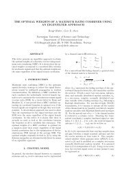
where a k is the fading amplitude, x k is the transmitted
channel symbol (in general complex), and z k is
complex AWGN. The fading amplitude is also in general
complex, but may be assumed to be real-valued
if perfect coherent detection is assumed at the receiver
end. We shall adopt this commonly used assumption
throughout this paper.
The fading amplitude a (for notational simplicity
we suppress the time dependence from now on) can be
described as a stochastic variable, whose distribution
we assume to be known. One particularly interesting
distribution is the Nakagami distribution [9]:
p A (a) = 2 ( m
) m
a 2m−1
Γ(m) 2σ 2 e −ma2 /2σ 2 (2)
Here, m> 1 2
is the Nakagami parameter, σ2 is the
fading amplitude variance, and Γ(x) is the gamma
function defined by
Γ(x) =
∫ ∞
0
y x−1 e −y dy, x > 0. (3)
The Nakagami distribution is of such interest because
it allows for modelling of a wide range of fading environments
by varying m, while yielding closed-form expressions
for many interesting features of the channel,
such as channel capacity. For m = 1 the model corresponds
to the Rayleigh fading model which is common
in mobile communications when there is no line-ofsight
(LOS) path between transmitter and receiver.
Increasing m will model less severe fading environments.
If a is Nakagami distributed, the CSNR will be
Gamma distributed as shown in Equation (4), γ and
γ being the instantaneous and expected CSNR respectively
[4].
( ) m m γ m−1
p γ (γ) =
(−m
γ Γ(m) exp γ )
, γ ≥ 0 (4)
γ
Under the assumption of perfect knowledge of the
channel state information (CSI) both on the receiver
and transmitter side, the maximum average spectral
efficiency (MASE), or channel capacity, of a Nakagami
multipath fading (NMF) channel has been shown
to be given by [1, Eq. 23]
m−1
∑
MASE = log 2 (e)e m/γ
k=0
( m
γ
) k (
Γ −k, m )
γ
(5)
where Γ(x, y) is the socalled complementary incomplete
Gamma function, which is commonly available
in numerical software such as MATLAB or Maple.
The MASE provides an ultimate performance benchmark
for the spectral efficiency of any practical communication
system communicating over this channel.
It has been shown that in order to efficiently exploit
the channel’s capacity over time without excessive
delay, a transmitter should switch between different
codes of different spectral efficiencies—in other words
adapt itself to the changes in channel quality as done
by adaptive coded modulation.
3. ACHIEVING CAPACITY ON AWGN
CHANNELS: LDPC CODES
In [10, 13] it is shown that carefully designed Low-
Density Parity Check (LDPC) codes almost attain
the Shannon channel capacity, i.e. the ultimate performance
limit, for AWGN channels with BPSK modulation.
The reason for this record-breaking performance
of LDPC codes can at least partly be explained by the
construction of the codes, to be explained below. According
to Shannon’s Channel Coding Theorem [11]
the channel capacity can be reached by using a code
consisting of very (in principle infinitely) long codewords
picked at random from some suitable distribution,
in combination with a decoder performing an
exhaustive nearest neighbour search.
Since a nearest neighbour search without any constraints
imposed is an NP-complete problem, such decoding
was assumed to be impossible in practice—
before the LDPC codes were invented by Gallager [3].
As implied by their name, limiting the space of possible
codes to LDPC codes provide an additional property
in the controlled sparseness (i.e., very low density
of non-zero bits in each column) of their parity check
matrices H. This reduces the number of equations to
be solved by the decoder and makes practical decoding
possible by means of iterative methods similar to
those used in turbo decoders.
To be more precise, an LDPC code is by definition
a linear error-correcting block code, which is specified
byaverysparseparitycheckmatrixH. A regular
LDPC code has an (N − K) × N H matrix with a
constant low number t of 1s in each column, placed at
random. An irregular LDPC code has a non-uniform
distribution of 1s in the rows and columns.
In any case, the parity check matrix may be generated
simply by running a binary random generator
(in the regular case, with probability t/N for emitting
1, and probability 1 − t/N for emitting 0). This is in
effect very similar to the code construction used by
Shannon in his proof of the Channel Coding Theorem,
but with the constraint of matrix sparseness added in
order to be able to find viable decoding algorithms.
If the matrix found does not provide a good code, the
random generator is simply run once more. Theoretically,
however, the probability of finding a good code
by such a random construction is very close to 1 if the
code length N is large.