Waveguides - ieeetsu
Waveguides - ieeetsu
Waveguides - ieeetsu

You also want an ePaper? Increase the reach of your titles
YUMPU automatically turns print PDFs into web optimized ePapers that Google loves.
256 Electromagnetic Waves & Antennas – S. J. Orfanidis – June 21, 2004<br />
8<br />
<strong>Waveguides</strong><br />
Rectangular waveguides are used routinely to transfer large amounts of microwave<br />
power at frequencies greater than 3 GHz. For example at 5 GHz, the transmitted power<br />
might be one megawatt and the attenuation only 4 dB/100 m.<br />
Optical fibers operate at optical and infrared frequencies, allowing a very wide bandwidth.<br />
Their losses are very low, typically, 0.2 dB/km. The transmitted power is of the<br />
order of milliwatts.<br />
8.1 Longitudinal-Transverse Decompositions<br />
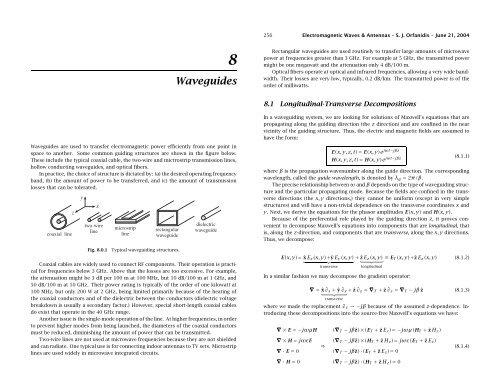
<strong>Waveguides</strong> are used to transfer electromagnetic power efficiently from one point in<br />
space to another. Some common guiding structures are shown in the figure below.<br />
These include the typical coaxial cable, the two-wire and mictrostrip transmission lines,<br />
hollow conducting waveguides, and optical fibers.<br />
In practice, the choice of structure is dictated by: (a) the desired operating frequency<br />
band, (b) the amount of power to be transferred, and (c) the amount of transmission<br />
losses that can be tolerated.<br />
Fig. 8.0.1<br />
Typical waveguiding structures.<br />
Coaxial cables are widely used to connect RF components. Their operation is practical<br />
for frequencies below 3 GHz. Above that the losses are too excessive. For example,<br />
the attenuation might be 3 dB per 100 m at 100 MHz, but 10 dB/100 m at 1 GHz, and<br />
50 dB/100 m at 10 GHz. Their power rating is typically of the order of one kilowatt at<br />
100 MHz, but only 200 W at 2 GHz, being limited primarily because of the heating of<br />
the coaxial conductors and of the dielectric between the conductors (dielectric voltage<br />
breakdown is usually a secondary factor.) However, special short-length coaxial cables<br />
do exist that operate in the 40 GHz range.<br />
Another issue is the single-mode operation of the line. At higher frequencies, in order<br />
to prevent higher modes from being launched, the diameters of the coaxial conductors<br />
must be reduced, diminishing the amount of power that can be transmitted.<br />
Two-wire lines are not used at microwave frequencies because they are not shielded<br />
and can radiate. One typical use is for connecting indoor antennas to TV sets. Microstrip<br />
lines are used widely in microwave integrated circuits.<br />
In a waveguiding system, we are looking for solutions of Maxwell’s equations that are<br />
propagating along the guiding direction (the z direction) and are confined in the near<br />
vicinity of the guiding structure. Thus, the electric and magnetic fields are assumed to<br />
have the form:<br />
E(x, y, z, t)= E(x, y)e jωt−jβz<br />
H(x, y, z, t)= H(x, y)e jωt−jβz (8.1.1)<br />
where β is the propagation wavenumber along the guide direction. The corresponding<br />
wavelength, called the guide wavelength, is denoted by λ g = 2π/β.<br />
The precise relationship between ω and β depends on the type of waveguiding structure<br />
and the particular propagating mode. Because the fields are confined in the transverse<br />
directions (the x, y directions,) they cannot be uniform (except in very simple<br />
structures) and will have a non-trivial dependence on the transverse coordinates x and<br />
y. Next, we derive the equations for the phasor amplitudes E(x, y) and H(x, y).<br />
Because of the preferential role played by the guiding direction z, it proves convenient<br />
to decompose Maxwell’s equations into components that are longitudinal, that<br />
is, along the z-direction, and components that are transverse, along the x, y directions.<br />
Thus, we decompose:<br />
E(x, y)= ˆx E x (x, y)+ŷ E y (x, y) + ẑ E z (x, y) ≡ E<br />
} {{ } } {{ } T (x, y)+ẑ E z (x, y) (8.1.2)<br />
transverse<br />
longitudinal<br />
In a similar fashion we may decompose the gradient operator:<br />
∇=ˆx ∂ x + ŷ ∂ y + ẑ ∂ z =∇ T + ẑ ∂ z =∇ T − jβ ẑ (8.1.3)<br />
} {{ }<br />
transverse<br />
where we made the replacement ∂ z →−jβ because of the assumed z-dependence. Introducing<br />
these decompositions into the source-free Maxwell’s equations we have:<br />
∇×E =−jωµH<br />
∇×H = jωɛE<br />
∇·E = 0<br />
∇·H = 0<br />
⇒<br />
(∇ T − jβẑ)×(E T + ẑ E z )=−jωµ(H T + ẑ H z )<br />
(∇ T − jβẑ)×(H T + ẑ H z )= jωɛ(E T + ẑ E z )<br />
(∇ T − jβẑ)·(E T + ẑ E z )= 0<br />
(∇ T − jβẑ)·(H T + ẑ H z )= 0<br />
(8.1.4)
www.ece.rutgers.edu/∼orfanidi/ewa 257<br />
258 Electromagnetic Waves & Antennas – S. J. Orfanidis – June 21, 2004<br />
where ɛ, µ denote the permittivities of the medium in which the fields propagate, for<br />
example, the medium between the coaxial conductors in a coaxial cable, or the medium<br />
within the hollow rectangular waveguide. This medium is assumed to be lossless for<br />
now.<br />
We note that ẑ · ẑ = 1, ẑ × ẑ = 0, ẑ · E T = 0, ẑ ·∇ T E z = 0 and that ẑ × E T and<br />
ẑ ×∇ T E z are transverse while ∇ T × E T is longitudinal. Indeed, we have:<br />
ẑ × E T = ẑ × (ˆx E x + ŷ E y )= ŷ E x − ˆx E y<br />
∇ T × E T = (ˆx ∂ x + ŷ ∂ y )×(ˆx E x + ŷ E y )= ẑ(∂ x E y − ∂ y E x )<br />
Using these properties and equating longitudinal and transverse parts in the two<br />
sides of Eq. (8.1.4), we obtain the equivalent set of Maxwell equations:<br />
∇ T E z × ẑ − jβ ẑ × E T =−jωµH T<br />
∇ T H z × ẑ − jβ ẑ × H T = jωɛE T<br />
∇ T × E T + jωµ ẑ H z = 0<br />
∇ T × H T − jωɛ ẑ E z = 0<br />
∇ T · E T − jβE z = 0<br />
∇ T · H T − jβH z = 0<br />
(8.1.5)<br />
Depending on whether both, one, or none of the longitudinal components are zero,<br />
we may classify the solutions as transverse electric and magnetic (TEM), transverse electric<br />
(TE), transverse magnetic (TM), or hybrid:<br />
E z = 0, H z = 0,<br />
E z = 0, H z ≠ 0,<br />
E z ≠ 0, H z = 0,<br />
E z ≠ 0, H z ≠ 0,<br />
TEM modes<br />
TE or H modes<br />
TM or E modes<br />
hybrid or HE or EH modes<br />
In the case of TEM modes, which are the dominant modes in two-conductor transmission<br />
lines such as the coaxial cable, the fields are purely transverse and the solution<br />
of Eq. (8.1.5) reduces to an equivalent two-dimensional electrostatic problem. We will<br />
discuss this case later on.<br />
In all other cases, at least one of the longitudinal fields E z ,H z is non-zero. It is then<br />
possible to express the transverse field components E T , H T in terms of the longitudinal<br />
ones, E z , H z .<br />
Forming the cross-product of the second of equations (8.1.5) with ẑ and using the<br />
BAC-CAB vector identity, ẑ × (ẑ × H T )= ẑ(ẑ · H T )−H T (ẑ · ẑ)= −H T , and similarly,<br />
ẑ × (∇ T H z × ẑ)=∇ T H z , we obtain:<br />
∇ T H z + jβH T = jωɛ ẑ × E T<br />
The solution of this system is:<br />
ẑ × E T =− jβ<br />
k 2 c<br />
H T =− jωɛ<br />
k 2 c<br />
ẑ ×∇ T E z − jωµ<br />
k 2 ∇ T H z<br />
c<br />
where we defined the so-called cutoff wavenumber k c by:<br />
ẑ ×∇ T E z − jβ<br />
(8.1.7)<br />
k 2 ∇ T H z<br />
c<br />
k 2 c = ω2 ɛµ − β 2 = ω2<br />
c − 2 β2 = k 2 − β 2 (cutoff wavenumber) (8.1.8)<br />
The quantity k = ω/c = ω √ ɛµ is the wavenumber a uniform plane wave would<br />
have in the propagation medium ɛ, µ.<br />
Although k 2 c stands for the difference ω2 ɛµ − β 2 , it turns out that the boundary<br />
conditions for each waveguide type force k 2 c to take on certain values, which can be<br />
positive, negative, or zero, and characterize the propagating modes. For example, in a<br />
dielectric waveguide k 2 c is positive inside the guide and negative outside it; in a hollow<br />
conducting waveguide k 2 c takes on certain quantized positive values; in a TEM line, k2 c<br />
is zero. Some related definitions are the cutoff frequency and the cutoff wavelength<br />
defined as follows:<br />
ω c = ck c , λ c = 2π (cutoff frequency and wavelength) (8.1.9)<br />
k c<br />
We can then express β in terms of ω and ω c ,orω in terms of β and ω c . Taking<br />
the positive square roots of Eq. (8.1.8), we have:<br />
√<br />
β = 1 √<br />
ω 2 − ω 2 c = ω √<br />
1 − ω2 c<br />
and ω = ω 2<br />
c<br />
c ω 2 c + β 2 c 2 (8.1.10)<br />
Often, Eq. (8.1.10) is expressed in terms of the wavelengths λ = 2π/k = 2πc/ω,<br />
λ c = 2π/k c , and λ g = 2π/β. It follows from k 2 = k 2 c + β 2 that<br />
1<br />
λ = 1 2 λ 2 + 1<br />
c λ 2 g<br />
λ<br />
⇒ λ g = √<br />
1 − λ2<br />
λ 2 c<br />
(8.1.11)<br />
Note that λ is related to the free-space wavelength λ 0 = 2πc 0 /ω = c 0 /f by the<br />
refractive index of the dielectric material λ = λ 0 /n.<br />
It is convenient at this point to introduce the transverse impedances for the TE and<br />
TM modes by the definitions:<br />
Thus, the first two of (8.1.5) may be thought of as a linear system of two equations<br />
in the two unknowns ẑ × E T and H T , that is,<br />
η TE = ωµ<br />
β = η ω βc , η TM = β ωɛ = η βc<br />
ω<br />
(TE and TM impedances) (8.1.12)<br />
β ẑ × E T − ωµH T = jẑ ×∇ T E z<br />
ωɛ ẑ × E T − βH T =−j∇ T H z<br />
(8.1.6)<br />
where the medium impedance is η = √ µ/ɛ, so that η/c = µ and ηc = 1/ɛ. We note the<br />
properties:
www.ece.rutgers.edu/∼orfanidi/ewa 259<br />
260 Electromagnetic Waves & Antennas – S. J. Orfanidis – June 21, 2004<br />
η TE η TM = η 2 η TE<br />
, =<br />
ω2<br />
∇ 2 T<br />
(8.1.13)<br />
=∇ T ·∇ T = ∂ 2 x + ∂2 y (8.1.18)<br />
η TM β 2 c 2 and we used the vectorial identities ∇ T ×∇ T E z = 0, ∇ T × (ẑ ×∇ T H z )= ẑ ∇ 2 T<br />
√<br />
H z, and<br />
∇<br />
Because βc/ω = 1 − ω 2 T · (ẑ ×∇ T H z )= 0.<br />
c/ω 2 , we can write also:<br />
It follows that in order to satisfy all of the last four of Maxwell’s equations (8.1.5), it<br />
√<br />
is necessary that the longitudinal fields E z (x, y), H z (x, y) satisfy the two-dimensional<br />
η<br />
η TE = √ , η TM = η 1 − ω2 c<br />
Helmholtz equations:<br />
(8.1.14)<br />
1 − ω2 ω 2 c<br />
ω 2 ∇ 2 T E z + kc 2E z = 0<br />
(Helmholtz equations) (8.1.19)<br />
With these definitions, we may rewrite Eq. (8.1.7) as follows:<br />
∇ 2 T H z + k 2 c H z = 0<br />
ẑ × E T =− jβ (ẑ )<br />
These equations are to be solved subject to the appropriate boundary conditions for<br />
×∇T<br />
k 2 E z + η TE ∇ T H z each waveguide type. Once, the fields E z ,H z are known, the transverse fields E T , H T are<br />
c<br />
H T =− jβ<br />
(8.1.15)<br />
computed from Eq. (8.1.16), resulting in a complete solution of Maxwell’s equations for<br />
( 1<br />
)<br />
k 2 ẑ ×∇ T E z +∇ T H z the guiding structure. To get the full x, y, z, t dependence of the propagating fields, the<br />
c η TM above solutions must be multiplied by the factor e jωt−jβz .<br />
Using the result ẑ × (ẑ × E T )=−E T , we solve for E T and H T :<br />
The cross-sections of practical waveguiding systems have either cartesian or cylindrical<br />
symmetry, such as the rectangular waveguide or the coaxial cable. Below, we<br />
E T =− jβ ( )<br />
summarize the form of the above solutions in the two types of coordinate systems.<br />
∇T<br />
k 2 E z − η TE ẑ ×∇ T H z<br />
c<br />
H T =− jβ (<br />
∇T<br />
k 2 H z + 1<br />
(transverse fields) (8.1.16)<br />
)<br />
Cartesian Coordinates<br />
ẑ ×∇ T E z<br />
c η TM<br />
The cartesian component version of Eqs. (8.1.16) and (8.1.19) is straightforward. Using<br />
An alternative and useful way of writing these equations is to form the following<br />
the identity ẑ ×∇ T H z = ŷ ∂ x H z − ˆx ∂ y H z , we obtain for the longitudinal components:<br />
linear combinations, which are equivalent to Eq. (8.1.6):<br />
(∂ 2 x + ∂2 y )E z + k 2 c E z = 0<br />
H T − 1 ẑ × E T = j η TM β ∇ (8.1.20)<br />
T H z<br />
(∂ 2 x + ∂ 2 y )H z + k 2 c H z = 0<br />
E T − η TE H T × ẑ = j (8.1.17)<br />
β ∇ Eq. (8.1.16) becomes for the transverse components:<br />
T E z<br />
So far we only used the first two of Maxwell’s equations (8.1.5) and expressed E T , H T<br />
E<br />
in terms of E z ,H z . Using (8.1.16), it is easily shown that the left-hand sides of the<br />
x =− jβ ( )<br />
∂x<br />
k 2 E z + η TE ∂ y H z H x =− jβ (<br />
∂x<br />
c<br />
remaining four of Eqs. (8.1.5) take the forms:<br />
∇ T × E T + jωµ ẑ H z = jωµ<br />
k 2 ẑ ( E y =− jβ ( ) , k 2 H z − 1 )<br />
∂ y E z<br />
c η TM<br />
∂y<br />
∇ 2 T H )<br />
z + k 2 k 2 E z − η TE ∂ x H z H y =− jβ (<br />
∂y<br />
c<br />
k 2 H z + 1<br />
(8.1.21)<br />
)<br />
∂ x E z<br />
c η TM<br />
cH z<br />
c<br />
∇ T × H T − jωɛ ẑ E z =− jωɛ<br />
k 2 ẑ ( ∇ 2 T E )<br />
z + kcE 2 Cylindrical Coordinates<br />
z<br />
c<br />
∇ T · E T − jβE z =− jβ (<br />
The relationship between cartesian and cylindrical coordinates is shown in Fig. 8.1.1.<br />
∇<br />
2<br />
kc<br />
2 T E z + k 2 c E z)<br />
From the triangle in the figure, we have x = ρ cos φ and y = ρ sin φ. The transverse<br />
∇ T · H T − jβH z =− jβ<br />
gradient and Laplace operator are in cylindrical coordinates:<br />
(<br />
∇<br />
2<br />
k 2 T H z + k 2 c H z)<br />
c<br />
∇ T = ˆρ ∂<br />
(<br />
where ∇ 2 T is the two-dimensional Laplacian operator: ∂ρ + ˆφ 1 ∂<br />
ρ ∂φ , ∇2 T = 1 ∂<br />
ρ ∂<br />
)<br />
ρ ∂ρ ∂ρ + 1 ∂ 2<br />
(8.1.22)<br />
ρ 2 ∂φ 2<br />
The Helmholtz equations (8.1.19) now read:
www.ece.rutgers.edu/∼orfanidi/ewa 261<br />
262 Electromagnetic Waves & Antennas – S. J. Orfanidis – June 21, 2004<br />
∫<br />
P T = P z dS ,<br />
S<br />
where P z = 1 2 Re(E × H∗ )·ẑ (8.2.1)<br />
It is easily verified that only the transverse components of the fields contribute to<br />
the power flow, that is, P z can be written in the form:<br />
Fig. 8.1.1<br />
Cylindrical coordinates.<br />
(<br />
1 ∂<br />
ρ ∂E )<br />
z<br />
+ 1 ∂ 2 E z<br />
ρ ∂ρ ∂ρ ρ 2 ∂φ + 2 k2 cE z = 0<br />
(<br />
1 ∂<br />
ρ ∂H )<br />
z<br />
+ 1 ∂ 2 H z<br />
ρ ∂ρ ∂ρ ρ 2 ∂φ + 2 k2 c H z = 0<br />
(8.1.23)<br />
P z = 1 2 Re(E T × H ∗ T )·ẑ (8.2.2)<br />
For waveguides with conducting walls, the transmission losses are due primarily to<br />
ohmic losses in (a) the conductors and (b) the dielectric medium filling the space between<br />
the conductors and in which the fields propagate. In dielectric waveguides the losses<br />
are due to absorption and scattering by imperfections.<br />
The transmission losses can be quantified by replacing the propagation wavenumber<br />
β by its complex-valued version β c = β − jα, where α is the attenuation constant. The<br />
z-dependence of all the field components is replaced by:<br />
Noting that ẑ × ˆρ = ˆφ and ẑ × ˆφ =−ˆρ, we obtain:<br />
ẑ ×∇ T H z = ˆφ(∂ ρ H z )−ˆρ 1 ρ (∂ φH z )<br />
The decomposition of a transverse vector is E T = ˆρE ρ + ˆφE φ . The cylindrical<br />
coordinates version of (8.1.16) are:<br />
E ρ =− jβ ( 1<br />
∂ρ<br />
k 2 E z − η TE<br />
c<br />
ρ ∂ )<br />
φH z<br />
E φ =− jβ ( 1<br />
k 2 c ρ ∂ ) ,<br />
φE z + η TE ∂ ρ H z<br />
H ρ =− jβ (<br />
∂ρ<br />
kc<br />
2 H z + 1<br />
η TM ρ ∂ )<br />
φE z<br />
H φ =− jβ ( 1<br />
kc<br />
2 ρ ∂ φH z − 1 )<br />
∂ ρ E z<br />
η TM<br />
(8.1.24)<br />
For either coordinate system, the equations for H T may be obtained from those of<br />
E T by a so-called duality transformation, that is, making the substitutions:<br />
E → H , H →−E , ɛ → µ, µ→ ɛ (duality transformation) (8.1.25)<br />
These imply that η → η −1 and η TE → η −1<br />
TM. Duality is discussed in greater detail in<br />
Sec. 16.2.<br />
8.2 Power Transfer and Attenuation<br />
With the field solutions at hand, one can determine the amount of power transmitted<br />
along the guide, as well as the transmission losses. The total power carried by the fields<br />
along the guide direction is obtained by integrating the z-component of the Poynting<br />
vector over the cross-sectional area of the guide:<br />
e −jβz → e −jβcz = e −(α+jβ)z = e −αz e −jβz (8.2.3)<br />
The quantity α is the sum of the attenuation constants arising from the various loss<br />
mechanisms. For example, if α d and α c are the attenuations due to the ohmic losses in<br />
the dielectric and in the conducting walls, then<br />
α = α d + α c (8.2.4)<br />
The ohmic losses in the dielectric can be characterized either by its loss tangent, say<br />
tan δ, or by its conductivity σ d —the two being related by σ d = ωɛ tan δ. The effective<br />
dielectric constant of the medium is then ɛ(ω)= ɛ − jσ d /ω = ɛ(1 − j tan δ). The<br />
corresponding complex-valued wavenumber β c is obtained by the replacement:<br />
β =<br />
√<br />
ω 2 µɛ − k 2 c → β c =<br />
√<br />
ω 2 µɛ(ω)−k 2 c<br />
For weakly conducting dielectrics, we may make the approximation:<br />
√<br />
β c =<br />
ω 2 µɛ ( 1 − j σ d<br />
ωɛ<br />
) √<br />
√<br />
− k<br />
2<br />
c = β 2 − jωµσ d = β 1 − j ωµσ d<br />
≃ β − j 1 β 2<br />
2 σ ωµ<br />
d<br />
β<br />
Recalling the definition η TE = ωµ/β, we obtain for the attenuation constant:<br />
α d = 1 2 σ dη TE = 1 2<br />
ω 2<br />
βc 2 tan δ =<br />
ω tan δ<br />
√1<br />
(dielectric losses) (8.2.5)<br />
2c − ω 2 c/ω 2<br />
which is similar to Eq. (2.7.2), but with the replacement η d → η TE .<br />
The conductor losses are more complicated to calculate. In practice, the following<br />
approximate procedure is adequate. First, the fields are determined on the assumption<br />
that the conductors are perfect.
www.ece.rutgers.edu/∼orfanidi/ewa 263<br />
264 Electromagnetic Waves & Antennas – S. J. Orfanidis – June 21, 2004<br />
Second, the magnetic fields on the conductor surfaces are determined and the corresponding<br />
induced surface currents are calculated by J s = ˆn × H, where ˆn is the outward<br />
normal to the conductor.<br />
Third, the ohmic losses per unit conductor area are calculated by Eq. (2.8.7). Figure<br />
8.2.1 shows such an infinitesimal conductor area dA = dl dz, where dl is along the<br />
cross-sectional periphery of the conductor. Applying Eq. (2.8.7) to this area, we have:<br />
dP loss<br />
dA<br />
= dP loss<br />
dldz = 1 2 R s|J s | 2 (8.2.6)<br />
where R s is the surface resistance of the conductor given by Eq. (2.8.4),<br />
√ √ √<br />
ωµ ωɛ<br />
R s =<br />
2σ = η 2σ = 1 2 δωµ , δ = 2<br />
= skin depth (8.2.7)<br />
ωµσ<br />
Integrating Eq. (8.2.6) around the periphery of the conductor gives the power loss per<br />
unit z-length due to that conductor. Adding similar terms for all the other conductors<br />
gives the total power loss per unit z-length:<br />
P ′ loss = dP loss<br />
dz<br />
∮<br />
∮<br />
= 1<br />
C a 2 R s|J s | 2 1<br />
dl +<br />
C b 2 R s|J s | 2 dl (8.2.8)<br />
One common property of all three types of modes is that the transverse fields E T , H T<br />
are related to each other in the same way as in the case of uniform plane waves propagating<br />
in the z-direction, that is, they are perpendicular to each other, their cross-product<br />
points in the z-direction, and they satisfy:<br />
H T = 1<br />
η T<br />
ẑ × E T (8.3.1)<br />
where η T is the transverse impedance of the particular mode type, that is, η, η TE ,η TM<br />
in the TEM, TE, and TM cases.<br />
Because of Eq. (8.3.1), the power flow per unit cross-sectional area described by the<br />
Poynting vector P z of Eq. (8.2.2) takes the simple form in all three cases:<br />
TEM modes<br />
P z = 1 2 Re(E T × H ∗ T )·ẑ = 1<br />
2η T<br />
|E T | 2 = 1 2 η T|H T | 2 (8.3.2)<br />
In TEM modes, both E z and H z vanish, and the fields are fully transverse. One can set<br />
E z = H z = 0 in Maxwell equations (8.1.5), or equivalently in (8.1.16), or in (8.1.17).<br />
From any point view, one obtains the condition k 2 c = 0, or ω = βc. For example, if<br />
the right-hand sides of Eq. (8.1.17) vanish, the consistency of the system requires that<br />
η TE = η TM , which by virtue of Eq. (8.1.13) implies ω = βc. It also implies that η TE ,η TM<br />
must both be equal to the medium impedance η. Thus, the electric and magnetic fields<br />
satisfy:<br />
H T = 1 η ẑ × E T (8.3.3)<br />
Fig. 8.2.1<br />
Conductor surface absorbs power from the propagating fields.<br />
These are the same as in the case of a uniform plane wave, except here the fields<br />
are not uniform and may have a non-trivial x, y dependence. The electric field E T is<br />
determined from the rest of Maxwell’s equations (8.1.5), which read:<br />
where C a and C b indicate the peripheries of the conductors. Finally, the corresponding<br />
attenuation coefficient is calculated from Eq. (2.6.22):<br />
α c = P′ loss<br />
(conductor losses) (8.2.9)<br />
2P T<br />
Equations (8.2.1)–(8.2.9) provide a systematic methodology by which to calculate the<br />
transmitted power and attenuation losses in waveguides. We will apply it to several<br />
examples later on.<br />
8.3 TEM, TE, and TM modes<br />
The general solution described by Eqs. (8.1.16) and (8.1.19) is a hybrid solution with nonzero<br />
E z and H z components. Here, we look at the specialized forms of these equations<br />
in the cases of TEM, TE, and TM modes.<br />
∇ T × E T = 0<br />
∇ T · E T = 0<br />
(8.3.4)<br />
These are recognized as the field equations of an equivalent two-dimensional electrostatic<br />
problem. Once this electrostatic solution is found, E T (x, y), the magnetic field<br />
is constructed from Eq. (8.3.3). The time-varying propagating fields will be given by<br />
Eq. (8.1.1), with ω = βc. (For backward moving fields, replace β by −β.)<br />
We explore this electrostatic point of view further in Sec. 9.1 and discuss the cases<br />
of the coaxial, two-wire, and strip lines. Because of the relationship between E T and H T ,<br />
the Poynting vector P z of Eq. (8.2.2) will be:<br />
P z = 1 2 Re(E T × H ∗ T )·ẑ = 1<br />
2η |E T| 2 = 1 2 η|H T| 2 (8.3.5)
www.ece.rutgers.edu/∼orfanidi/ewa 265<br />
266 Electromagnetic Waves & Antennas – S. J. Orfanidis – June 21, 2004<br />
TE modes<br />
TE modes are characterized by the conditions E z = 0 and H z ≠ 0. It follows from the<br />
second of Eqs. (8.1.17) that E T is completely determined from H T , that is, E T = η TE H T ×ẑ.<br />
The field H T is determined from the second of (8.1.16). Thus, all field components<br />
for TE modes are obtained from the equations:<br />
∇T 2 H z + k 2 cH z = 0<br />
H T =− jβ<br />
k 2 ∇ T H z<br />
c<br />
E T = η TE H T × ẑ<br />
(TE modes) (8.3.6)<br />
The relationship of E T and H T is identical to that of uniform plane waves propagating<br />
in the z-direction, except the wave impedance is replaced by η TE . The Poynting vector<br />
of Eq. (8.2.2) then takes the form:<br />
P z = 1 2 Re(E T × H ∗ T )·ẑ = 1 |E T | 2 = 1 2η TE 2 η TE|H T | 2 = 1 2 η β 2<br />
TE<br />
k 4 |∇ T H z | 2 (8.3.7)<br />
c<br />
The cartesian coordinate version of Eq. (8.3.6) is:<br />
∇ 2 T E z + k 2 c E z = 0<br />
E T =− jβ<br />
k 2 ∇ T E z<br />
c<br />
H T = 1 ẑ × E T<br />
η TM<br />
(TM modes) (8.3.10)<br />
Again, the relationship of E T and H T is identical to that of uniform plane waves<br />
propagating in the z-direction, but the wave impedance is now η TM . The Poynting vector<br />
takes the form:<br />
P z = 1 2 Re(E T × H ∗ T )·ẑ = 1 |E T | 2 = 1 β 2<br />
2η TM 2η TM k 4 |∇ T E z | 2 (8.3.11)<br />
c<br />
8.4 Rectangular <strong>Waveguides</strong><br />
Next, we discuss in detail the case of a rectangular hollow waveguide with conducting<br />
walls, as shown in Fig. 8.4.1. Without loss of generality, we may assume that the lengths<br />
a, b of the inner sides satisfy b ≤ a. The guide is typically filled with air, but any other<br />
dielectric material ɛ, µ may be assumed.<br />
(∂ 2 x + ∂ 2 y)H z + k 2 cH z = 0<br />
H x =− jβ ∂ x H z ,<br />
H y =− jβ ∂ y H z<br />
(8.3.8)<br />
k 2 c<br />
k 2 c<br />
And, the cylindrical coordinate version:<br />
(<br />
1 ∂<br />
ρ ∂H )<br />
z<br />
+ 1 ∂ 2 H z<br />
ρ ∂ρ ∂ρ ρ 2 ∂φ + 2 k2 c H z = 0<br />
H ρ =− jβ ∂H z<br />
k 2 , H φ =− jβ 1 ∂H z<br />
(8.3.9)<br />
c ∂ ρ k 2 c ρ ∂ φ<br />
E ρ = η TE H φ , E φ =−η TE H ρ<br />
where we used H T × ẑ = (ˆρH ρ + ˆφH φ )×ẑ =−ˆφH ρ + ˆρH φ .<br />
TM modes<br />
TM modes have H z = 0 and E z ≠ 0. It follows from the first of Eqs. (8.1.17) that H T is<br />
completely determined from E T , that is, H T = η −1<br />
TMẑ × E T. The field E T is determined<br />
from the first of (8.1.16), so that all field components for TM modes are obtained from<br />
the following equations, which are dual to the TE equations (8.3.6):<br />
Fig. 8.4.1<br />
Rectangular waveguide.<br />
The simplest and dominant propagation mode is the so-called TE 10 mode and depends<br />
only on the x-coordinate (of the longest side.) Therefore, we begin by looking<br />
for solutions of Eq. (8.3.8) that depend only on x. In this case, the Helmholtz equation<br />
reduces to:<br />
∂ 2 xH z (x)+k 2 cH z (x)= 0<br />
The most general solution is a linear combination of cos k c x and sin k c x. However,<br />
only the former will satisfy the boundary conditions. Therefore, the solution is:<br />
H z (x)= H 0 cos k c x (8.4.1)<br />
where H 0 is a (complex-valued) constant. Because there is no y-dependence, it follows<br />
from Eq. (8.3.8) that ∂ y H z = 0, and hence H y = 0 and E x = 0. It also follows that:<br />
H x (x)= − jβ<br />
k 2 c<br />
∂ x H z =− jβ<br />
k 2 (−k c )H 0 sin k c x = jβ H 0 sin k c x ≡ H 1 sin k c x<br />
c<br />
k c
www.ece.rutgers.edu/∼orfanidi/ewa 267<br />
268 Electromagnetic Waves & Antennas – S. J. Orfanidis – June 21, 2004<br />
Then, the corresponding electric field will be:<br />
where we defined the constants:<br />
E y (x)= −η TE H x (x)= −η TE<br />
jβ<br />
k c<br />
H 0 sin k c x ≡ E 0 sin k c x<br />
H 1 = jβ<br />
k c<br />
H 0<br />
E 0 =−η TE H 1 =−η TE<br />
jβ<br />
k c<br />
H 0 =−jη ω ω c<br />
H 0<br />
(8.4.2)<br />
where we used η TE = ηω/βc. In summary, the non-zero field components are:<br />
H z (x)= H 0 cos k c x<br />
H x (x)= H 1 sin k c x<br />
E y (x)= E 0 sin k c x<br />
⇒<br />
H z (x, y, z, t)= H 0 cos k c xe jωt−jβz<br />
H x (x, y, z, t)= H 1 sin k c xe jωt−jβz<br />
E y (x, y, z, t)= E 0 sin k c xe jωt−jβz (8.4.3)<br />
Assuming perfectly conducting walls, the boundary conditions require that there be<br />
no tangential electric field at any of the wall sides. Because the electric field is in the<br />
y-direction, it is normal to the top and bottom sides. But, it is parallel to the left and<br />
right sides. On the left side, x = 0, E y (x) vanishes because sin k c x does. On the right<br />
side, x = a, the boundary condition requires:<br />
E y (a)= E 0 sin k c a = 0 ⇒ sin k c a = 0<br />
This requires that k c a be an integral multiple of π:<br />
k c a = nπ ⇒ k c = nπ (8.4.4)<br />
a<br />
These are the so-called TE n0 modes. The corresponding cutoff frequency ω c = ck c ,<br />
f c = ω c /2π, and wavelength λ c = 2π/k c = c/f c are:<br />
ω c = cnπ<br />
a , f c = cn<br />
2a , λ c = 2a (TE n0 modes) (8.4.5)<br />
n<br />
The dominant mode is the one with the lowest cutoff frequency or the longest cutoff<br />
wavelength, that is, the mode TE 10 having n = 1. It has:<br />
k c = π a , ω c = cπ a , f c = c<br />
2a , λ c = 2a (TE 10 mode) (8.4.6)<br />
Fig. 8.4.2 depicts the electric field E y (x)= E 0 sin k c x = E 0 sin(πx/a) of this mode<br />
as a function of x.<br />
Fig. 8.4.2<br />
8.5 Higher TE and TM modes<br />
Electric field inside a rectangular waveguide.<br />
To construct higher modes, we look for solutions of the Helmholtz equation that are<br />
factorable in their x and y dependence:<br />
Then, Eq. (8.3.8) becomes:<br />
H z (x, y)= F(x)G(y)<br />
F ′′ (x)G(y)+F(x)G ′′ (y)+k 2 cF(x)G(y)= 0 ⇒ F′′ (x)<br />
F(x) + G′′ (y)<br />
G(y) + k2 c = 0 (8.5.1)<br />
Because these must be valid for all x, y (inside the guide), the F- and G-terms must<br />
be constants, independent of x and y. Thus, we write:<br />
F ′′ (x)<br />
F(x) =−k2 x ,<br />
G ′′ (y)<br />
G(y) =−k2 y<br />
F ′′ (x)+k 2 xF(x)= 0 , G ′′ (y)+k 2 yG(y)= 0 (8.5.2)<br />
where the constants k 2 x and k2 y are constrained from Eq. (8.5.1) to satisfy:<br />
k 2 c = k 2 x + k 2 y (8.5.3)<br />
The most general solutions of (8.5.2) that will satisfy the TE boundary conditions are<br />
cos k x x and cos k y y. Thus, the longitudinal magnetic field will be:<br />
H z (x, y)= H 0 cos k x x cos k y y (TE nm modes) (8.5.4)<br />
It then follows from the rest of the equations (8.3.8) that:<br />
H x (x, y) = H 1 sin k x x cos k y y<br />
H y (x, y) = H 2 cos k x x sin k y y<br />
where we defined the constants:<br />
H 1 = jβk x<br />
k 2 c<br />
H 0 ,<br />
H 2 = jβk y<br />
k 2 c<br />
H 0<br />
or<br />
E x (x, y) = E 1 cos k x x sin k y y<br />
E y (x, y) = E 2 sin k x x cos k y y<br />
(8.5.5)<br />
E 1 = η TE H 2 = jη ωk y<br />
ω c k c<br />
H 0 ,<br />
E 2 =−η TE H 1 =−jη ωk x<br />
ω c k c<br />
H 0
www.ece.rutgers.edu/∼orfanidi/ewa 269<br />
The boundary conditions are that E y vanish on the right wall, x = a, and that E x<br />
vanish on the top wall, y = b, that is,<br />
E y (a, y)= E 0y sin k x a cos k y y = 0 , E x (x, b)= E 0x cos k x x sin k y b = 0<br />
The conditions require that k x a and k y b be integral multiples of π:<br />
k x a = nπ , k y b = mπ ⇒ k x = nπ a , k y = mπ<br />
(8.5.6)<br />
b<br />
These √ correspond to the TE nm modes. Thus, the cutoff wavenumbers of these modes<br />
k c = k 2 x + k 2 y take on the quantized values:<br />
√ ( ) nπ 2 ( ) mπ 2<br />
k c =<br />
+<br />
(TE nm modes) (8.5.7)<br />
a b<br />
The cutoff frequencies f nm = ω c /2π = ck c /2π and wavelengths λ nm = c/f nm are:<br />
f nm = c<br />
√ ( n<br />
2a<br />
) 2 ( ) m 2<br />
+ , λ nm =<br />
2b<br />
√ ( n<br />
2a<br />
1<br />
) 2 ( ) (8.5.8)<br />
m<br />
2<br />
+<br />
2b<br />
The TE 0m modes are similar to the TE n0 modes, but with x and a replaced by y and<br />
b. The family of TM modes can also be constructed in a similar fashion from Eq. (8.3.10).<br />
Assuming E z (x, y)= F(x)G(y), we obtain the same equations (8.5.2). Because E z<br />
is parallel to all walls, we must now choose the solutions sin k x and sin k y y. Thus, the<br />
longitudinal electric fields is:<br />
E z (x, y)= E 0 sin k x x sin k y y (TM nm modes) (8.5.9)<br />
The rest of the field components can be worked out from Eq. (8.3.10) and one finds<br />
that they are given by the same expressions as (8.5.5), except now the constants are<br />
determined in terms of E 0 :<br />
E 1 =− jβk x<br />
k 2 c<br />
E 0 ,<br />
E 2 =− jβk y<br />
k 2 c<br />
H 1 =− 1<br />
η TM<br />
E 2 = jωk y<br />
ω c k c<br />
1<br />
η E 0 , H 2 = 1<br />
η TM<br />
E 1 =− jωk x<br />
ω c k c<br />
1<br />
η H 0<br />
where we used η TM = ηβc/ω. The boundary conditions on E x ,E y are the same as<br />
before, and in addition, we must require that E z vanish on all walls.<br />
These conditions imply that k x ,k y will be given by Eq. (8.5.6), except both n and m<br />
must be non-zero (otherwise E z would vanish identically.) Thus, the cutoff frequencies<br />
and wavelengths are the same as in Eq. (8.5.8).<br />
Waveguide modes can be excited by inserting small probes at the beginning of the<br />
waveguide. The probes are chosen to generate an electric field that resembles the field<br />
of the desired mode.<br />
E 0<br />
270 Electromagnetic Waves & Antennas – S. J. Orfanidis – June 21, 2004<br />
8.6 Operating Bandwidth<br />
All waveguiding systems are operated in a frequency range that ensures that only the<br />
lowest mode can propagate. If several modes can propagate simultaneously, † one has<br />
no control over which modes will actually be carrying the transmitted signal. This may<br />
cause undue amounts of dispersion, distortion, and erratic operation.<br />
A mode with cutoff frequency ω c will propagate only if its frequency is ω ≥ ω c ,<br />
or λ
www.ece.rutgers.edu/∼orfanidi/ewa 271<br />
272 Electromagnetic Waves & Antennas – S. J. Orfanidis – June 21, 2004<br />
Fig. 8.6.1<br />
Operating bandwidth in rectangular waveguides.<br />
where<br />
H 1 = jβ H 0 , E 0 =−η TE H 1 =−jη ω H 0 (8.7.2)<br />
k c ω c<br />
The Poynting vector is obtained from the general result of Eq. (8.3.7):<br />
P z = 1<br />
2η TE<br />
|E T | 2 = 1<br />
2η TE<br />
|E y (x)| 2 = 1<br />
2η TE<br />
|E 0 | 2 sin 2 k c x<br />
The transmitted power is obtained by integrating P z over the cross-sectional area<br />
of the guide:<br />
widest bandwidth, we also require to have the maximum power transmitted, the dimension<br />
b must be chosen to be as large as possible, that is, b = a/2. Most practical guides<br />
follow these side proportions.<br />
If there is a “canonical” guide, it will have b = a/2 and be operated at a frequency<br />
that lies in the middle of the operating band [f c , 2f c ], that is,<br />
f = 1.5f c = 0.75 c (8.6.1)<br />
a<br />
Table 8.6.1 lists some standard air-filled rectangular waveguides with their naming<br />
designations, inner side dimensions a, b in inches, cutoff frequencies in GHz, minimum<br />
and maximum recommended operating frequencies in GHz, power ratings, and attenuations<br />
in dB/m (the power ratings and attenuations are representative over each operating<br />
band.) We have chosen one example from each microwave band.<br />
name a b f c f min f max band P α<br />
WR-510 5.10 2.55 1.16 1.45 2.20 L 9 MW 0.007<br />
WR-284 2.84 1.34 2.08 2.60 3.95 S 2.7 MW 0.019<br />
WR-159 1.59 0.795 3.71 4.64 7.05 C 0.9 MW 0.043<br />
WR-90 0.90 0.40 6.56 8.20 12.50 X 250 kW 0.110<br />
WR-62 0.622 0.311 9.49 11.90 18.00 Ku 140 kW 0.176<br />
WR-42 0.42 0.17 14.05 17.60 26.70 K 50 kW 0.370<br />
WR-28 0.28 0.14 21.08 26.40 40.00 Ka 27 kW 0.583<br />
WR-15 0.148 0.074 39.87 49.80 75.80 V 7.5 kW 1.52<br />
WR-10 0.10 0.05 59.01 73.80 112.00 W 3.5 kW 2.74<br />
Table 8.6.1 Characteristics of some standard air-filled rectangular waveguides.<br />
8.7 Power Transfer, Energy Density, and Group Velocity<br />
Next, we calculate the time-averaged power transmitted in the TE 10 mode. We also calculate<br />
the energy density of the fields and determine the velocity by which electromagnetic<br />
energy flows down the guide and show that it is equal to the group velocity. We recall<br />
that the non-zero field components are:<br />
H z (x)= H 0 cos k c x, H x (x)= H 1 sin k c x, E y (x)= E 0 sin k c x (8.7.1)<br />
Noting the definite integral,<br />
∫ a<br />
∫ b<br />
P T =<br />
0 0<br />
1<br />
2η TE<br />
|E 0 | 2 sin 2 k c x dxdy<br />
∫ a<br />
∫ a<br />
sin 2 k c xdx= sin<br />
2( πx ) a dx =<br />
0<br />
0 a 2<br />
√<br />
and using η TE = ηω/βc = η/ 1 − ω 2 c/ω 2 , we obtain:<br />
(8.7.3)<br />
√<br />
P T = 1 |E 0 | 2 ab = 1<br />
4η TE 4η |E 0| 2 ab 1 − ω2 c<br />
ω 2 (transmitted power) (8.7.4)<br />
We may also calculate the distribution of electromagnetic energy along the guide, as<br />
measured by the time-averaged energy density. The energy densities of the electric and<br />
magnetic fields are:<br />
w e = 1 2 Re( 1 2 ɛE · E∗) = 1 4 ɛ|E y| 2<br />
w m = 1 2 Re( 1 2 µH · H∗) = 1 4 µ( |H x | 2 +|H z | 2)<br />
Inserting the expressions for the fields, we find:<br />
w e = 1 4 ɛ|E 0| 2 sin 2 k c x, w m = 1 4 µ( |H 1 | 2 sin 2 k c x +|H 0 | 2 cos 2 k c x )<br />
Because these quantities represent the energy per unit volume, if we integrate them<br />
over the cross-sectional area of the guide, we will obtain the energy distributions per<br />
unit z-length. Using the integral (8.7.3) and an identical one for the cosine case, we find:<br />
W ′ e = ∫ a<br />
0<br />
W ′ m = ∫ a<br />
0<br />
∫ b<br />
0<br />
∫ b<br />
0<br />
∫ a<br />
∫ b<br />
W e (x, y) dxdy =<br />
0 0<br />
1<br />
4 ɛ|E 0| 2 sin 2 k c x dxdy = 1 8 ɛ|E 0| 2 ab<br />
1<br />
4 µ( |H 1 | 2 sin 2 k c x +|H 0 | 2 cos 2 k c x ) dxdy = 1 8 µ( |H 1 | 2 +|H 0 | 2) ab
www.ece.rutgers.edu/∼orfanidi/ewa 273<br />
274 Electromagnetic Waves & Antennas – S. J. Orfanidis – June 21, 2004<br />
Although these expressions look different, they are actually equal, W e ′ = W m ′ . Indeed,<br />
using the property β 2 /k 2 c + 1 = (β2 + k 2 c )/k2 c = k2 /k 2 c = ω2 /ω 2 c and the relationships<br />
between the constants in (8.7.1), we find:<br />
µ ( |H 1 | 2 +|H 0 | 2) = µ ( |H 0 | 2 β2<br />
k 2 +|H 0 | 2) = µ|H 0 | 2 ω2<br />
c<br />
ωc<br />
2 = µ η |E 0| 2 = ɛ|E 2 0 | 2<br />
The equality of the electric and magnetic energies is a general property of waveguiding<br />
systems. We also encountered it in Sec. 2.3 for uniform plane waves. The total<br />
energy density per unit length will be:<br />
The field expressions (8.4.3) were derived assuming the boundary conditions for<br />
perfectly conducting wall surfaces. The induced surface currents on the inner walls of<br />
the waveguide are given by J s = ˆn × H, where the unit vector ˆn is ±ˆx and ±ŷ on the<br />
left/right and bottom/top walls, respectively.<br />
The surface currents and tangential magnetic fields are shown in Fig. 8.8.1. In particular,<br />
on the bottom and top walls, we have:<br />
W ′ = W ′ e + W′ m = 2W′ e = 1 4 ɛ|E 0| 2 ab (8.7.5)<br />
According to the general relationship between flux, density, and transport velocity<br />
given in Eq. (1.5.2), the energy transport velocity will be the ratio v en = P T /W ′ . Using<br />
Eqs. (8.7.4) and (8.7.5) and noting that 1/ηɛ = 1/ √ µɛ = c, we find:<br />
√<br />
v en = P T<br />
W ′ = c 1 − ω2 c<br />
(energy transport velocity) (8.7.6)<br />
ω 2<br />
This is equal to the group velocity of the propagating mode. For any dispersion<br />
relationship between ω and β, the group and phase velocities are defined by<br />
v gr = dω<br />
dβ ,<br />
v ph = ω β<br />
(group and phase velocities) (8.7.7)<br />
For uniform plane waves and TEM transmission lines, we have ω = βc, so that v gr =<br />
v ph = c. For a rectangular waveguide, we have ω 2 = ω 2 c + β2 c 2 . Taking differentials of<br />
both sides, we find 2ωdω = 2c 2 βdβ, which gives:<br />
√<br />
v gr = dω<br />
dβ = βc2<br />
ω<br />
= c 1 − ω2 c<br />
ω 2 (8.7.8)<br />
where we used Eq. (8.1.10). Thus, the energy transport velocity is equal to the group<br />
velocity, v en = v gr . We note that v gr = βc 2 /ω = c 2 /v ph ,or<br />
Fig. 8.8.1<br />
Currents on waveguide walls.<br />
J s =±ŷ × H =±ŷ × (ˆx H x + ẑH z )=±(−ẑ H x + ˆx H z )=±(−ẑ H 1 sin k c x + ˆx H 0 cos k c x)<br />
Similarly, on the left and right walls:<br />
J s =±ˆx × H =±ˆx × (ˆx H x + ẑH z )=∓ŷ H z =∓ŷ H 0 cos k c x<br />
At x = 0 and x = a, this gives J s =∓ŷ(±H 0 )= ŷ H 0 . Thus, the magnitudes of the<br />
surface currents are on the four walls:<br />
{<br />
|J s | 2 |H0 | 2 , (left and right walls)<br />
=<br />
|H 0 | 2 cos 2 k c x +|H 1 | 2 sin 2 k c x, (top and bottom walls)<br />
The power loss per unit z-length is obtained from Eq. (8.2.8) by integrating |J s | 2<br />
around the four walls, that is,<br />
P ′ loss = 2 1 2 R s<br />
∫ a<br />
0<br />
|J s | 2 dx + 2 1 2 R s<br />
∫ b<br />
0<br />
|J s | 2 dy<br />
v gr v ph = c 2 (8.7.9)<br />
The energy or group velocity satisfies v gr ≤ c, whereas v ph ≥ c. Information transmission<br />
down the guide is by the group velocity and, consistent with the theory of<br />
relativity, it is less than c.<br />
8.8 Power Attenuation<br />
In this section, we calculate the attenuation coefficient due to the ohmic losses of the<br />
conducting walls following the procedure outlined in Sec. 8.2. The losses due to the<br />
filling dielectric can be determined from Eq. (8.2.5).<br />
∫ a<br />
(<br />
= R s |H0 | 2 cos 2 k c x +|H 1 | 2 sin 2 k c x ) ∫ b<br />
dx + R s |H 0 | 2 dy<br />
0<br />
0<br />
a (<br />
= R s |H0 | 2 +|H 1 | 2) + R s b|H 0 | 2 = R sa (<br />
|H0 | 2 +|H 1 | 2 + 2b 2<br />
2<br />
a |H 0| 2)<br />
Using |H 0 | 2 +|H 1 | 2 =|E 0 | 2 /η 2 from Sec. 8.7, and |H 0 | 2 = (|E 0 | 2 /η 2 )ωc/ω 2 2 , which<br />
follows from Eq. (8.4.2), we obtain:<br />
P ′ loss = R sa|E 0 |<br />
(1 2<br />
+ 2b )<br />
ω 2 c<br />
2η 2 a ω 2<br />
The attenuation constant is computed from Eqs. (8.2.9) and (8.7.4):
www.ece.rutgers.edu/∼orfanidi/ewa 275<br />
276 Electromagnetic Waves & Antennas – S. J. Orfanidis – June 21, 2004<br />
which gives:<br />
α c = R s<br />
ηb<br />
α c = P′ loss<br />
2P T<br />
=<br />
(<br />
1 + 2b a<br />
√<br />
)<br />
ω 2 c<br />
ω 2<br />
R s a|E 0 | 2<br />
(1 + 2b 2η 2 a<br />
√<br />
2 1<br />
4η |E 0| 2 ab<br />
)<br />
ω 2 c<br />
ω 2<br />
1 − ω2 c<br />
ω 2<br />
1 − ω2 c<br />
ω 2 (attenuation of TE 10 mode) (8.8.1)<br />
This is in units of nepers/m. Its value in dB/m is obtained by α dB = 8.686α c . For a<br />
given ratio a/b, α c increases with decreasing b, thus the smaller the guide dimensions,<br />
the larger the attenuation. This trend is noted in Table 8.6.1.<br />
The main tradeoffs in a waveguiding system are that as the operating frequency f<br />
increases, the dimensions of the guide must decrease in order to maintain the operating<br />
band f c ≤ f ≤ 2f c , but then the attenuation increases and the transmitted power<br />
decreases as it is proportional to the guide’s area.<br />
Example 8.8.1: Design a rectangular air-filled waveguide to be operated at 5 GHz, then, redesign<br />
it to be operated at 10 GHz. The operating frequency must lie in the middle of the<br />
operating band. Calculate the guide dimensions, the attenuation constant in dB/m, and<br />
the maximum transmitted power assuming the maximum electric field is one-half of the<br />
dielectric strength of air. Assume copper walls with conductivity σ = 5.8×10 7 S/m.<br />
Solution: If f is in the middle of the operating band, f c ≤ f ≤ 2f c , where f c = c/2a, then<br />
f = 1.5f c = 0.75c/a. Solving for a, wefind<br />
a = 0.75c<br />
f<br />
0.75×30 GHz cm<br />
= = 4.5 cm<br />
5<br />
For maximum power transfer, we require b = a/2 = 2.25 cm. Because ω = 1.5ω c ,we<br />
have ω c /ω = 2/3. Then, Eq. (8.8.1) gives α c = 0.037 dB/m. The dielectric strength of air<br />
is 3 MV/m. Thus, the maximum allowed electric field in the guide is E 0 = 1.5 MV/m. Then,<br />
Eq. (8.7.4) gives P T = 1.12 MW.<br />
At 10 GHz, because f is doubled, the guide dimensions are halved, a = 2.25 and b = 1.125<br />
cm. Because R s depends on f like f 1/2 , it will increase by a factor of √ 2. Then, the factor<br />
R s /b will increase by a factor of 2 √ 2. Thus, the attenuation will increase to the value<br />
α c = 0.037 · 2 √ 2 = 0.104 dB/m. Because the area ab is reduced by a factor of four, so<br />
will the power, P T = 1.12/4 = 0.28 MW = 280 kW.<br />
The results of these two cases are consistent with the values quoted in Table 8.6.1 for the<br />
C-band and X-band waveguides, WR-159 and WR-90.<br />
⊓⊔<br />
Example 8.8.2: WR-159 Waveguide. Consider the C-band WR-159 air-filled waveguide whose<br />
characteristics were listed in Table 8.6.1. Its inner dimensions are a = 1.59 and b = a/2 =<br />
0.795 inches, or, equivalently, a = 4.0386 and b = 2.0193 cm.<br />
α (dB/m)<br />
0.1<br />
0.08<br />
0.06<br />
0.04<br />
0.02<br />
The cutoff frequency of the TE 10 mode is f c = c/2a = 3.71 GHz. The maximum operating<br />
bandwidth is the interval [f c , 2f c ]= [3.71, 7.42] GHz, and the recommended interval is<br />
[4.64, 7.05] GHz.<br />
Assuming copper walls with conductivity σ = 5.8×10 7 S/m, the calculated attenuation<br />
constant α c from Eq. (8.8.1) is plotted in dB/m versus frequency in Fig. 8.8.2.<br />
Attenuation Coefficient<br />
bandwidth<br />
0<br />
0 1 2 3 4 5 6 7 8 9 10 11 12<br />
f (GHz)<br />
Fig. 8.8.2<br />
P T (MW)<br />
1.5<br />
1<br />
0.5<br />
Power Transmitted<br />
bandwidth<br />
0<br />
0 1 2 3 4 5 6 7 8 9 10 11 12<br />
f (GHz)<br />
Attenuation constant and transmitted power in a WR-159 waveguide.<br />
The power transmitted P T is calculated from Eq. (8.7.4) assuming a maximum breakdown<br />
voltage of E 0 = 1.5 MV/m, which gives a safety factor of two over the dielectric breakdown<br />
of air of 3 MV/m. The power in megawatt scales is plotted in Fig. 8.8.2.<br />
√<br />
Because of the factor 1 − ω 2 c/ω 2 in the denominator of α c and the numerator of P T ,<br />
the attenuation constant becomes very large near the cutoff frequency, while the power is<br />
almost zero. A physical explanation of this behavior is given in the next section. ⊓⊔<br />
8.9 Reflection Model of Waveguide Propagation<br />
An intuitive model for the TE 10 mode can be derived by considering a TE-polarized<br />
uniform plane wave propagating in the z-direction by obliquely bouncing back and forth<br />
between the left and right walls of the waveguide, as shown in Fig. 8.9.1.<br />
If θ is the angle of incidence, then the incident and reflected (from the right wall)<br />
wavevectors will be:<br />
k = ˆx k x + ẑ k z = ˆx k cos θ + ẑ k sin θ<br />
k ′ =−ˆx k x + ẑ k z =−ˆx k cos θ + ẑ k sin θ<br />
The electric and magnetic fields will be the sum of an incident and a reflected component<br />
of the form:<br />
E = ŷ E 1 e −jk·r + ŷ E ′ 1e −jk′·r = ŷ E 1 e −jkxx e −jkzz + ŷ E ′ 1e jkxx e −jkzz = E 1 + E ′ 1<br />
H = 1 η ˆk × E 1 + 1 η ˆk ′ × E ′ 1
www.ece.rutgers.edu/∼orfanidi/ewa 277<br />
278 Electromagnetic Waves & Antennas – S. J. Orfanidis – June 21, 2004<br />
Fig. 8.9.1<br />
Reflection model of TE 10 mode.<br />
where the electric field was taken to be polarized in the y direction. These field expressions<br />
become component-wise:<br />
E y = ( E 1 e −jkxx + E ′ 1e jkxx) e −jkzz<br />
H x =− 1 η sin θ( E 1 e −jkxx + E ′ 1e jkxx) e −jkzz<br />
H z = 1 η cos θ( E 1 e −jkxx − E ′ 1e jkxx) e −jkzz (8.9.1)<br />
The boundary condition on the left wall, x = 0, requires that E 1 + E ′ 1 = 0. We may write<br />
therefore, E 1 =−E ′ 1 = jE 0 /2. Then, the above expressions simplify into:<br />
E y = E 0 sin k x xe −jkzz<br />
H x =− 1 η sin θE 0 sin k x xe −jkzz<br />
H z = j η cos θE 0 cos k x xe −jkzz (8.9.2)<br />
The boundary condition on the right wall requires sin k x a = 0, which gives rise to<br />
the same condition as (8.4.4), that is, k c a = nπ.<br />
This model clarifies also the meaning of the group velocity. The plane wave is bouncing<br />
left and right with the speed of light c. However, the component of this velocity in<br />
the z-direction will be v z = c sin θ. This is equal to the group velocity. Indeed, it follows<br />
from Eq. (8.9.3) that:<br />
v z = c sin θ = c 1 − ω2 c<br />
ω = v 2 gr (8.9.5)<br />
Eq. (8.9.3) implies also that at ω = ω c , we have sin θ = 0, or θ = 0, that is, the wave<br />
is bouncing left and right at normal incidence, creating a standing wave, and does not<br />
propagate towards the z-direction. Thus, the transmitted power is zero and this also<br />
implies, through Eq. (8.2.9), that α c will be infinite.<br />
On the other hand, for very large frequencies, ω ≫ ω c , the angle θ will tend to 90 o ,<br />
causing the wave to zoom through guide almost at the speed of light.<br />
8.10 Resonant Cavities<br />
Cavity resonators are metallic enclosures that can trap electromagnetic fields. The<br />
boundary conditions on the cavity walls force the fields to exist only at certain quantized<br />
resonant frequencies. For highly conducting walls, the resonances are extremely sharp,<br />
having a very high Q of the order of 10,000.<br />
Because of their high Q, cavities can be used not only to efficiently store electromagnetic<br />
energy at microwave frequencies, but also to act as precise oscillators and to<br />
perform precise frequency measurements.<br />
Fig. 8.10.1 shows a rectangular cavity with z-length equal to l formed by replacing<br />
the sending and receiving ends of a waveguide by metallic walls. A forward-moving wave<br />
will bounce back and forth from these walls, resulting in a standing-wave pattern along<br />
the z-direction.<br />
√<br />
These are identical to Eq. (8.4.3) provided we identify β with k z and k c with k x ,as<br />
shown in Fig. 8.9.1. It follows from the wavevector triangle in the figure that the angle<br />
of incidence θ will be given by cos θ = k x /k = k c /k, or,<br />
cos θ = ω c<br />
ω ,<br />
sin θ = √<br />
1 − ω2 c<br />
ω 2 (8.9.3)<br />
The ratio of the transverse components, −E y /H x , is the transverse impedance, which<br />
is recognized to be η TE . Indeed, we have:<br />
η TE =− E y<br />
=<br />
η<br />
H x sin θ = √<br />
η<br />
1 − ω2 c<br />
ω 2 (8.9.4)<br />
Fig. 8.10.1<br />
Rectangular cavity resonator (and induced wall currents for the TE n0p mode.)<br />
Because the tangential components of the electric field must vanish at the end-walls,<br />
these walls must coincide with zero crossings of the standing wave, or put differently, an<br />
integral multiple of half-wavelengths must fit along the z-direction, that is, l = pλ g /2 =<br />
pπ/β, orβ = pπ/l, where p is a non-zero integer. For the same reason, the standingwave<br />
patterns along the transverse directions require a = nλ x /2 and b = mλ y /2, or
www.ece.rutgers.edu/∼orfanidi/ewa 279<br />
280 Electromagnetic Waves & Antennas – S. J. Orfanidis – June 21, 2004<br />
k x = nπ/a and k y = mπ/b. Thus, all three cartesian components of the wave vector<br />
√<br />
are quantized, and therefore, so is the frequency of the wave ω = c kx 2 + k 2 y + β 2 :<br />
√ ( ) nπ 2 ( ) mπ 2 ( ) pπ 2<br />
ω nmp = c + +<br />
(resonant frequencies) (8.10.1)<br />
a b l<br />
Such modes are designated as TE nmp or TM nmp . For simplicity, we consider the case<br />
TE n0p . Eqs. (8.3.6) also describe backward-moving waves if one replaces β by −β, which<br />
also changes the sign of η TE = ηω/βc. Starting with a linear combination of forward<br />
and backward waves in the TE n0 mode, we obtain the field components:<br />
H z (x, z) = H 0 cos k c x ( Ae −jβz + Be jβz) ,<br />
H x (x, z) = jH 1 sin k c x ( Ae −jβz − Be jβz) , H 1 = β k c<br />
H 0<br />
E y (x, z) =−jE 0 sin k c x ( Ae −jβz + Be jβz) , E 0 = ω ω c<br />
ηH 0<br />
(8.10.2)<br />
where ω c = ck c . By requiring that E y (x, z) have z-dependence of the form sin βz, the<br />
coefficients A, B must be chosen as A =−B = j/2. Then, Eq. (8.10.2) specializes into:<br />
H z (x, z) = H 0 cos k c x sin βz ,<br />
H x (x, z) =−H 1 sin k c x cos βz , H 1 = β k c<br />
H 0<br />
E y (x, z) =−jE 0 sin k c x sin βz , E 0 = ω ω c<br />
ηH 0<br />
(8.10.3)<br />
As expected, the vanishing of E y (x, z) on the front/back walls, z = 0 and z = l, and<br />
on the left/right walls, x = 0 and x = a, requires the quantization conditions: β = pπ/l<br />
and k c = nπ/a. The Q of the resonator can be calculated from its definition:<br />
Q = ω<br />
W<br />
(8.10.4)<br />
P loss<br />
where W is the total time-averaged energy stored within the cavity volume and P loss is<br />
the total power loss due to the wall ohmic losses (plus other losses, such as dielectric<br />
losses, if present.) The ratio ∆ω = P loss /W is usually identified as the 3-dB width of the<br />
resonance centered at frequency ω. Therefore, we may write Q = ω/∆ω.<br />
It is easily verified that the electric and magnetic energies are equal, therefore, W<br />
may be calculated by integrating the electric energy density over the cavity volume:<br />
W = 2W e = 2 1 ∫<br />
ɛ|E y (x, z)| 2 dx dy dz = 1 ∫ a<br />
∫ b<br />
∫ l<br />
4 vol 2 ɛ|E 0| 2 sin 2 k c x cos 2 βz dx dy dz<br />
0 0 0<br />
[ ]<br />
= 1 8 ɛ|E 0| 2 (abl)= 1 8 µ|H 0| 2 ω2<br />
ω 2 (abl)= 1 k<br />
c 8 µ |H 0| 2 2<br />
c + β 2<br />
k 2 (abl)<br />
c<br />
where we used the following definite integrals (valid because k c = nπ/a, β = pπ/l):<br />
∫ a<br />
∫ a<br />
sin 2 k c xdx= cos 2 k c xdx= a ∫ l<br />
∫ l<br />
0<br />
0<br />
2 , sin 2 βz dz = cos 2 βz dz = l (8.10.5)<br />
0<br />
0<br />
2<br />
The ohmic losses are calculated from Eq. (8.2.6), integrated over all six cavity sides.<br />
The surface currents induced on the walls are related to the tangential magnetic fields<br />
by J s = ˆn × H tan . The directions of these currents are shown in Fig. 8.10.1. Specifically,<br />
we find for the currents on the six sides:<br />
⎧<br />
⎪⎨<br />
H0 2 sin2 βz<br />
(left & right)<br />
|J s | 2 = H0 2 ⎪⎩<br />
cos2 k c x sin 2 βz + H1 2 sin2 k c x cos 2 βz (top & bottom)<br />
H1 2 sin2 k c x<br />
(front & back)<br />
The power loss can be computed by integrating the loss per unit conductor area,<br />
Eq. (8.2.6), over the six wall sides, or doubling the answer for the left, top, and front<br />
sides. Using the integrals (8.10.5), we find:<br />
P loss = 1 ∫<br />
2 R s |J s | 2 dA = R s<br />
[H 2 bl<br />
0<br />
walls<br />
2 + (H2 0 + H1) 2 al ]<br />
4 + ab<br />
H2 1<br />
2<br />
[<br />
]<br />
= 1 (8.10.6)<br />
4 R sH0<br />
2 l(2b + a)+ β2<br />
k 2 a(2b + l)<br />
c<br />
where we substituted H1 2 = H0β 2 2 /kc 2 . It follows that the Q-factor will be:<br />
Q = ω<br />
W = ωµ (k 2 c + β2 )(abl)<br />
P loss 2R s k 2 cl(2b + a)+β 2 a(2b + l)<br />
For the TE n0p mode we have β = pπ/l and k c = nπ/a. Using Eq. (8.2.7) to replace<br />
R s in terms of the skin depth δ, we find:<br />
n 2<br />
Q = 1 a + p2<br />
2 l 2<br />
δ n 2 ( 2<br />
a 2 a + 1 ) (<br />
+ p2 2<br />
b l 2 l + 1 ) (8.10.7)<br />
b<br />
The lowest resonant frequency corresponds to n = p = 1. For a cubic cavity, a =<br />
b = l, the Q and the lowest resonant frequency are:<br />
Q = a<br />
3δ , ω 101 = cπ√ 2<br />
a<br />
, f 101 = ω 2π = c<br />
a √ 2<br />
(8.10.8)<br />
For an air-filled cubic cavity with a = 3 cm, we find f 101 = 7.07 GHz, δ = 7.86×10 −5<br />
cm, and Q = 12724. As in waveguides, cavities can be excited by inserting small probes<br />
that generate fields resembling a particular mode.<br />
8.11 Dielectric Slab <strong>Waveguides</strong><br />
A dielectric slab waveguide is a planar dielectric sheet or thin film of some thickness,<br />
say 2a, as shown in Fig. 8.11.1. Wave propagation in the z-direction is by total internal<br />
reflection from the left and right walls of the slab. Such waveguides provide simple<br />
models for the confining mechanism of waves propagating in optical fibers.
www.ece.rutgers.edu/∼orfanidi/ewa 281<br />
282 Electromagnetic Waves & Antennas – S. J. Orfanidis – June 21, 2004<br />
k 2 c = k2 0n 2 1 − β 2<br />
−α 2 c = k2 0n 2 2 − β 2<br />
⇒<br />
k 2 c = k2 0n 2 1 − β 2<br />
α 2 c = β2 − k 2 0n 2 2<br />
(8.11.3)<br />
Similarly, Eqs. (8.11.2) read:<br />
∂ 2 x H z(x)+k 2 c H z(x)= 0 for |x| ≤a<br />
∂ 2 x H z(x)−α 2 c H z(x)= 0 for |x| ≥a<br />
(8.11.4)<br />
Fig. 8.11.1<br />
Dielectric slab waveguide.<br />
The propagating fields are confined primarily inside the slab, however, they also<br />
exist as evanescent waves outside it, decaying exponentially with distance from the slab.<br />
Fig. 8.11.1 shows a typical electric field pattern as a function of x.<br />
For simplicity, we assume that the media to the left and right of the slab are the<br />
same. To guarantee total internal reflection, the dielectric constants inside and outside<br />
the slab must satisfy ɛ 1 >ɛ 2 , and similarly for the refractive indices, n 1 >n 2 .<br />
We look for TE solutions that depend only on the x coordinate. The cutoff wavenumber<br />
k c appearing in the Helmholtz equation for H z (x) depends on the dielectric constant<br />
of the propagation medium, k 2 c = ω2 ɛµ−β 2 . Therefore, k 2 c takes different values inside<br />
and outside the guide:<br />
k 2 c1 = ω 2 ɛ 1 µ 0 − β 2 = ω 2 ɛ 0 µ 0 n 2 1 − β 2 = k 2 0n 2 1 − β 2<br />
k 2 c2 = ω 2 ɛ 2 µ 0 − β 2 = ω 2 ɛ 0 µ 0 n 2 2 − β 2 = k 2 0n 2 2 − β 2<br />
(inside)<br />
(outside)<br />
(8.11.1)<br />
where k 0 = ω/c 0 is the free-space wavenumber. We note that ω, β are the same inside<br />
and outside the guide. This follows from matching the tangential fields at all times t<br />
and all points z along the slab walls. The corresponding Helmholtz equations in the<br />
regions inside and outside the guide are:<br />
∂ 2 xH z (x)+k 2 c1H z (x)= 0 for |x| ≤a<br />
(8.11.2)<br />
∂ 2 x H z(x)+k 2 c2H z (x)= 0 for |x| ≥a<br />
Inside the slab, the solutions are sin k c1 x and cos k c1 x, and outside, sin k c2 x and<br />
cos k c2 x, or equivalently, e ±jkc2x . In order for the waves to remain confined in the near<br />
vicinity of the slab, the quantity k c2 must be imaginary, for if it is real, the fields would<br />
propagate at large x distances from the slab (they would correspond to the rays refracted<br />
from the inside into the outside.)<br />
If we set k c2 =−jα c , the solutions outside will be e ±αcx .Ifα c is positive, then only<br />
the solution e −αcx is physically acceptable to the right of the slab, x ≥ a, and only e αcx<br />
to the left, x ≤−a. Thus, the fields attenuate exponentially with the transverse distance<br />
x, and exist effectively within a skin depth distance 1/α c from the slab. Setting k c1 = k c<br />
and k c2 =−jα c , Eqs. (8.11.1) become in this new notation:<br />
The two solutions sin k c x and cos k c x inside the guide give rise to the so-called even<br />
and odd TE modes (referring to the even-ness or oddness of the resulting electric field.)<br />
For the even modes, the solutions of Eqs. (8.11.4) have the form:<br />
⎧<br />
H ⎪⎨ 1 sin k c x, if −a ≤ x ≤ a<br />
H z (x)= H 2 e −αcx , if x ≥ a<br />
⎪⎩<br />
H 3 e αcx , if x ≤−a<br />
(8.11.5)<br />
The corresponding x-components are obtained by applying Eq. (8.3.8) using the appropriate<br />
value for k 2 c , that is, k2 c2 =−α 2 c outside and k2 c1 = k 2 c inside:<br />
⎧<br />
⎪⎨<br />
H x (x)=<br />
− jβ<br />
k 2 ∂ x H z (x)= − jβ H 1 cos k c x, if −a ≤ x ≤ a<br />
c<br />
k c<br />
− jβ<br />
−α 2 ∂ x H z (x)= − jβ H 2 e −αcx , if x ≥ a<br />
c<br />
α c<br />
(8.11.6)<br />
⎪⎩ − jβ<br />
−α 2 ∂ x H z (x)= jβ H 3 e αcx , if x ≥ a<br />
c<br />
α c<br />
The electric fields are E y (x)= −η TE H x (x), where η TE = ωµ 0 /β is the same inside<br />
and outside the slab. Thus, the electric field has the form:<br />
⎧<br />
E ⎪⎨ 1 cos k c x, if −a ≤ x ≤ a<br />
E y (x)= E 2 e −αcx , if x ≥ a<br />
(even TE modes) (8.11.7)<br />
⎪⎩<br />
E 3 e αcx , if x ≤−a<br />
where we defined the constants:<br />
E 1 = jβ η TE H 1 , E 2 = jβ η TE H 2 , E 3 =− jβ η TE H 3 (8.11.8)<br />
k c α c α c<br />
The boundary conditions state that the tangential components of the magnetic and<br />
electric fields, that is, H z ,H x ,E y , are continuous across the dielectric interfaces at x =<br />
−a and x = a. Because E y =−η TE H x and η TE is the same in both media, the continuity<br />
of E y follows from the continuity of H x . The continuity of H z at x = a and x =−a<br />
implies that:<br />
H 1 sin k c a = H 2 e −αca and − H 1 sin k c a = H 3 e −αca (8.11.9)<br />
Similarly, the continuity of H x implies (after canceling a factor of −jβ):
www.ece.rutgers.edu/∼orfanidi/ewa 283<br />
284 Electromagnetic Waves & Antennas – S. J. Orfanidis – June 21, 2004<br />
1<br />
H 1 cos k c a = 1 H 2 e −αca and<br />
k c α c<br />
Eqs. (8.11.9) and (8.11.10) imply:<br />
1<br />
k c<br />
H 1 cos k c a =− 1 α c<br />
H 3 e −αca (8.11.10)<br />
⎧<br />
E ⎪⎨ 1 cos k c x, if −a ≤ x ≤ a<br />
E y (x)= E 1 cos k c ae −αc(x−a) , if x ≥ a<br />
⎪⎩<br />
E 1 cos k c ae αc(x+a) , if x ≤−a<br />
(even TE modes) (8.11.19)<br />
H 2 =−H 3 = H 1 e αca sin k c a = H 1 e αca α c<br />
cos k c a (8.11.11)<br />
k c<br />
Similarly, we find for the electric field constants:<br />
E 2 = E 3 = E 1 e αca cos k c a = E 1 e αca k c<br />
sin k c a (8.11.12)<br />
α c<br />
The consistency of the last equations in (8.11.11) or (8.11.12) requires that:<br />
cos k c a = k c<br />
sin k c a ⇒ α c = k c tan k c a (8.11.13)<br />
α c<br />
For the odd TE modes, we have for the solutions of Eq. (8.11.4):<br />
The resulting electric field is:<br />
⎧<br />
H ⎪⎨ 1 cos k c x, if −a ≤ x ≤ a<br />
H z (x)= H 2 e −αcx , if x ≥ a<br />
⎪⎩<br />
H 3 e αcx , if x ≤−a<br />
⎧<br />
E ⎪⎨ 1 sin k c x, if −a ≤ x ≤ a<br />
E y (x)= E 2 e −αcx , if x ≥ a<br />
⎪⎩<br />
E 3 e αcx , if x ≤−a<br />
The boundary conditions imply in this case:<br />
(8.11.14)<br />
(odd TE modes) (8.11.15)<br />
H 2 = H 3 = H 1 e αca cos k c a =−H 1 e αca α c<br />
sin k c a (8.11.16)<br />
k c<br />
and, for the electric field constants:<br />
E 2 =−E 3 = E 1 e αca sin k c a =−E 1 e αca k c<br />
cos k c a (8.11.17)<br />
α c<br />
The consistency of the last equation requires:<br />
α c =−k c cot k c a (8.11.18)<br />
We note that the electric fields E y (x) given by Eqs. (8.11.7) and (8.11.15) are even or<br />
odd functions of x for the two families of modes. Expressing E 2 and E 3 in terms of E 1 ,<br />
we summarize the forms of the electric fields in the two cases:<br />
⎧<br />
E ⎪⎨ 1 sin k c x, if −a ≤ x ≤ a<br />
E y (x)= E 1 sin k c ae −αc(x−a) , if x ≥ a<br />
⎪⎩<br />
−E 1 sin k c ae αc(x+a) , if x ≤−a<br />
(odd TE modes) (8.11.20)<br />
Given the operating frequency ω, Eqs. (8.11.3) and (8.11.13) or (8.11.18) provide three<br />
equations in the three unknowns k c ,α c ,β. To solve them, we add the two equations<br />
(8.11.3) to eliminate β:<br />
α 2 c + k 2 c = k 2 0(n 2 1 − n 2 2)= ω2<br />
c 2 (n 2 1 − n 2 2) (8.11.21)<br />
0<br />
Next, we discuss the numerical solutions of these equations. Defining the dimensionless<br />
quantities u = k c a and v = α c a, we may rewrite Eqs. (8.11.13), (8.11.18), and<br />
(8.11.21) in the equivalent forms:<br />
v = u tan u<br />
v 2 + u 2 = R 2 (even modes) ,<br />
where R is the normalized frequency variable:<br />
R = k 0 aN A = ωa<br />
c 0<br />
v =−u cot u<br />
v 2 + u 2 = R 2 (odd modes) (8.11.22)<br />
N A = 2πfa N A = 2πa<br />
c 0 λ N A (8.11.23)<br />
√<br />
where N A = n 2 1 − n 2 2 is the numerical aperture of the slab and λ = c 0/f, the free-space<br />
wavelength.<br />
Because the functions tan u and cot u have many branches, there may be several<br />
possible solution pairs u, v for each value of R. These solutions are obtained at the<br />
intersections of the curves v = u tan u and v =−u cot u with the circle of radius R,<br />
that is, v 2 + u 2 = R 2 . Fig. 8.11.2 shows the solutions for various values of the radius R<br />
corresponding to various values of ω.<br />
It is evident from the figure that for small enough R, that is, 0 ≤ R
www.ece.rutgers.edu/∼orfanidi/ewa 285<br />
286 Electromagnetic Waves & Antennas – S. J. Orfanidis – June 21, 2004<br />
v = u tan(u − R m )<br />
v 2 + u 2 = R 2 (mth mode) (8.11.29)<br />
If one had an approximate solution u, v for the mth mode, one could refine it by using<br />
Newton’s method, which converges very fast provided it is close to the true solution. Just<br />
such an approximate solution, accurate to within one percent of the true solution, was<br />
given by Lotspeich [464]. Without going into the detailed justification of this method,<br />
the approximation is as follows:<br />
u = R m + w 1 (m)u 1 (m)+w 2 (m)u 2 (m) , m = 0, 1,...,M (8.11.30)<br />
where u 1 (m), u 2 (m) are approximate solutions near and far from the cutoff R m , and<br />
w 1 (m), w 2 (m) are weighting factors:<br />
Fig. 8.11.2<br />
Even and odd TE modes at different frequencies.<br />
Given a value of R, we determine M as that integer satisfying Eq. (8.11.24), or, M ≤<br />
2R/π
www.ece.rutgers.edu/∼orfanidi/ewa 287<br />
288 Electromagnetic Waves & Antennas – S. J. Orfanidis – June 21, 2004<br />
[be,kc,ac,fc,err] = dguide(f,a,n1,n2,Nit);<br />
% dielectric slab guide<br />
where f is in GHz, a in cm, and β, k c ,α c in cm −1 . The quantity f c is the vector of<br />
the M + 1 cutoff frequencies defined by the branch edges R m = mπ/2, that is, R m =<br />
ω m aN A /c 0 = 2πf m aN A /c 0 = mπ/2, or,<br />
f m = mc 0<br />
, m = 0, 1,...,M (8.11.35)<br />
4aN A<br />
The meaning of f m is that there are m + 1 propagating modes for each f is in the<br />
interval f m ≤ f
www.ece.rutgers.edu/∼orfanidi/ewa 289<br />
8.2 It is desired to design an air-filled rectangular waveguide such that (a) it operates only in the<br />
TE 10 mode with the widest possible bandwidth, (b) it can transmit the maximum possible<br />
power, and (c) the operating frequency is 12 GHz and it lies in the middle of the operating<br />
band. What are the dimensions of the guide in cm?<br />
8.3 An air-filled rectangular waveguide is used to transfer power to a radar antenna. The guide<br />
must meet the following specifications: The two lowest modes are TE 10 and TE 20 . The operating<br />
frequency is 3 GHz and must lie exactly halfway between the cutoff frequencies of<br />
these two modes. The maximum electric field within the guide may not exceed, by a safety<br />
margin of 3, the breakdown field of air 3 MV/m.<br />
a. Determine the smallest dimensions a, b for such a waveguide, if the transmitted power<br />
is required to be 1 MW.<br />
b. What are the dimensions a, b if the transmitted power is required to be maximum?<br />
What is that maximum power in MW?<br />
8.4 It is desired to design an air-filled rectangular waveguide operating at 5 GHz, whose group<br />
velocity is 0.8c. What are the dimensions a, b of the guide (in cm) if it is also required to carry<br />
maximum power and have the widest possible bandwidth? What is the cutoff frequency of<br />
the guide in GHz and the operating bandwidth?<br />
8.5 Show the following relationship between guide wavelength and group velocity in an arbitrary<br />
air-filled waveguide: v g λ g = cλ , where λ g = 2π/β and λ is the free-space wavelength.<br />
Moreover, show that the λ and λ g are related to the cutoff wavelength λ c by:<br />
1<br />
λ = 1 2 λ 2 + 1<br />
g λ 2 c<br />
8.6 Determine the four lowest modes that can propagate in a WR-159 and a WR-90 waveguide.<br />
Calculate the cutoff frequencies (in GHz) and cutoff wavelengths (in cm) of these modes.<br />
8.7 An air-filled WR-90 waveguide is operated at 9 GHz. Calculate the maximum power that<br />
can be transmitted without causing dielectric breakdown of air. Calculate the attenuation<br />
constant in dB/m due to wall ohmic losses. Assume copper walls.<br />
8.8 A rectangular waveguide has sides a, b such that b ≤ a/2. Determine the cutoff wavelength<br />
λ c of this guide. Show that the operating wavelength band of the lowest mode is 0.5λ c ≤<br />
λ ≤ λ c . Moreover, show that the allowed range of the guide wavelength is λ g ≥ λ c / √ 3.<br />
8.9 The TE 10 mode operating bandwidth of an air-filled waveguide is required to be 4–7 GHz.<br />
What are the dimensions of the guide?<br />
8.10 Computer Experiment: WR-159 Waveguide. Reproduce the two graphs of Fig. 8.8.2.<br />
8.11 Computer Experiment: Dielectric Slab Waveguide. Using the MATLAB functions dslab and<br />
dguide, write a program that reproduces all the results and graphs of Examples 8.11.1 and<br />
8.11.2.<br />
8.12 A TM mode is propagated along a waveguide of arbitrary but uniform cross section. Assume<br />
perfectly conducting walls.<br />
a. Show that the E z (x, y) component satisfies:<br />
∫<br />
∫<br />
|∇E z | 2 dS = k 2 c |E z | 2 dS<br />
S<br />
S<br />
b. Using the above result, show that the energy velocity is equal to the group velocity.