IT3105 AI Programming: Speech Recognition Lecture Notes

IT3105 AI Programming: Speech Recognition
Lecture Notes
Helge Langseth, IT Vest 310
Version 1.04 – April 13, 2011
ThisnoteaimsatintroducingtherequiredbackgroundforbuildingabasicSpeech
Recognition System (SRS). The topics that will be covered are i) basic properties
of speech, and ii) a brief recap of how to build probabilistic temporal models,
in particular Hidden Markov Models (HMMs) with the associated inference and
learning algorithm.
The “classic” reference for everybody working with probabilistic speech recognition,
and also a very important reference for this project, is Lawrence R. Rabiner:
“A Tutorial on Hidden Markov Models and Selected Applications in Speech Recognition”,
which can be downloaded from the course’s webpage. The paper gives a
broad account of probabilistic speech recognition, with focus on the internals of
HMM inference and learning. It contains more information than we will need in
this project, but if you read (and understand!) pp. 257–266 (until “IV. Types
of HMMs”), Subsection “IV.A. Continuous observation densities in HMMs” (p.
267) and Subsection “V.A Scaling” (pp. 272–273) you should be well covered for
now. The main goal of this note is thus to get you up to speed so that you can
understand the paper by Rabiner, and implement the techniques discussed there.
Those of you who have taken the “Methods in AI”-course should already be familiarwiththeHMMs,
butifyouhave forgottenallaboutit, Irecommendtolook
at Chapter 15 of Russell & Norvig: “Artificial Intelligence, A Modern Approach”
again, as R&N give a good and fairly readable account of these models. Be
warned that the notation and terminology differ somewhat between R&N’s book
and Rabiner’s paper, though. Note also that when R&N’s Section 15.6 describes
the practicalities of how to build an SRS, the approach taken there is a bit more
labour-intensive than the one we will pursue, and I therefore recommend to not
confuse yourself by reading R&N’s Section 15.6 now. If you are not familiar with
HMMs I recommend to read Russell&Norvig, Chapters 13–15 before continuing
on this note.
1

In addition to the already mentioned reference, there is a wealth of information
about SRSs available online, including a number of fancy demonstrations that
you may find motivating to take a look at.
In this project we will make an SRS that recognises single-word-speech, and we
will assume that the speech stems from a limited vocabulary. Compared to what
the state-of-the-art SRSs today can do, this is a very simplified problem. The
reason for choosing to consider only a stripped-down version of thegeneral speech
recognition problem is that we can now avoid looking at refined acoustic models
andlanguagegrammars; bothofwhich constituteimportantpartsof“real”SRSs.
Basically, this means that our approach will be data intensive, and we will not
spend time on the linguistic side of things. However, we will still meet some of
the same challenges as state-of-the-art SRSs have to tackle, and I therefore hope
that theproblem will be aninteresting challenge even thoughit isabit simplified.
1 Sound signals and how to represent them
Let us start by looking at how speech is created. We focus attention to vocalisation,
meaning sounds made by humans using the mouth, nose, and throat. A
vocalisation is made up by a series of utterances; one utterance being the stream
of speech between two periods of silence. As we are concerned by speech of single
words, an utterance given to the SRS will always contain exactly one word (and
separation of words is therefore not required). When a word is spoken, the task of
generating the speech is divided into generating the separate phonemes. People
do this by using lips, tongue, jaw, vocal cords, and lungs. When we move the
lungs we create an air flow through the other articulators, which again makes
the sound. As the air flows past the vocal cords, tension applied to the vocal
cords causes the creation of a tone or pitch. Sound is transported through air
as variations in pressure, and this is what is detected by the human ear. Humans
can distinguish sounds in the range from30 Hz to about 20 kHz, with best results
for sounds at about 1 kHz.
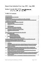
Figure 1 plots some example utterances. The amplitude of the speech signal
is plotted as a function of time, and the topmost plot shows the speech signal
representing the vocalisation of “Start [pause] Stop [pause] Left [pause] Right”.
The four plots below give the speech signal for each utterance separately. The
scale on the x-axis is time in seconds, the y-axis gives the amplitude of the signal
after normalisation. The important thing to take home from Figure 1 is that
speech signals are dynamic – they change over time, and to be able to recognise
one example of speech as being an utterance of a particular word, we must take
this dynamic nature of the speech signal into account when we build our SRS.
2

1
0.5
0
Signal
−0.5
−1
−1.5
0 0.5 1 1.5 2 2.5 3 3.5 4
Time (s)
Signal −− Start
0.8
0.6
0.4
0.2
0
−0.2
−0.4
−0.6
−0.8
0 0.05 0.1 0.15 0.2 0.25
Time (s)
Signal −− Stop
0.4
0.3
0.2
0.1
0
−0.1
−0.2
−0.3
−0.4
−0.5
−0.6
0 0.02 0.04 0.06 0.08 0.1 0.12 0.14
Time (s)
0.8
0.4
0.6
0.3
0.4
0.2
Signal −− Left
0.2
0
−0.2
Signal −− Right
0.1
0
−0.1
−0.4
−0.2
−0.6
−0.3
−0.8
0 0.02 0.04 0.06 0.08 0.1 0.12 0.14 0.16 0.18
Time (s)
−0.4
0 0.02 0.04 0.06 0.08 0.1 0.12 0.14 0.16 0.18 0.2
Time (s)
Figure 1: This is the raw signal of the the utterance of the four words “Start”,
“Stop”, “Left”, and “Right”.
3

0 0.02 0.04 0.06 0.08 0.1 0.12 0.14 0.16 0.18 0.2
0.5
0.5
0.5
0.4
0.4
0.4
0.3
0.3
0.3
Signal from file − LEFT(1)
0.2
0.1
0
−0.1
−0.2
Signal from file − LEFT(2)
0.2
0.1
0
−0.1
−0.2
Signal from file − LEFT(3)
0.2
0.1
0
−0.1
−0.2
−0.3
−0.3
−0.3
−0.4
−0.4
−0.4
−0.5
Time (s)
−0.5
0 0.02 0.04 0.06 0.08 0.1 0.12 0.14 0.16 0.18 0.2
Time (s)
−0.5
0 0.02 0.04 0.06 0.08 0.1 0.12 0.14 0.16 0.18 0.2
Time (s)
0.5
0.5
0.5
0.4
0.4
0.4
0.3
0.3
0.3
Signal from file − LEFT(4)
0.2
0.1
0
−0.1
−0.2
Signal from file − LEFT(5)
0.2
0.1
0
−0.1
−0.2
Signal from file − LEFT(6)
0.2
0.1
0
−0.1
−0.2
−0.3
−0.3
−0.3
−0.4
−0.4
−0.4
−0.5
0 0.02 0.04 0.06 0.08 0.1 0.12 0.14 0.16 0.18 0.2
Time (s)
−0.5
0 0.02 0.04 0.06 0.08 0.1 0.12 0.14 0.16 0.18 0.2
Time (s)
−0.5
0 0.02 0.04 0.06 0.08 0.1 0.12 0.14 0.16 0.18 0.2
Time (s)
Figure 2: Several utterances of the word “Left”.
The representation of different words in Figure 1 look rather different, and this
may give us the idea to use the sound signal itself as our representation of an
utterance. Recognition would in this case amount to comparing a new speech
signal to prototypical examples of earlier recorded speech, and classify the new
utterance to the class being most “similar” in these terms. Before ascribing to
that strategy, though, we must investigate the robustness of the speech signal
representation. We say that a speech representation is robust if it is (almost)
identical each time the same word is spoken. If we have a robust speech representation,
this will obviously be beneficial when the speech is to be recognised.
Consider Figure 2, where six utterances of the word “Left” are shown. Although
the speech examples come from the same speaker, there are differences in the
maximum amplitude and the “overall look” of the signals; symptoms of lacking
robustness in this representation.
Weinvestigate thisfurther inFigure3, wherethe(time-dependent) averagesignal
of 35 utterances of the word “Left” is shown, together with the time-dependent
95% confidence interval of the 35 signals. As we see, the structure in the signal is
completely overshadowed by the variability, and the raw signal thereby appears
unsuitable as a representation in the SRS. We therefore proceed by trying to
“robustify” the signal; a process described in Figure 4. At the beginning, the
speech signal is continuous in time as shown in the topmost part of the figure.
This signal is fed to the computer via a microphone, which captures the pressure
wave of the original speech and translates it into an analogue electrical signal.
At that point the sound is a real-valued function of continuous time, and the
signal can in principle be saved exactly as it was using a tape system. However,
although we have deliberately disregarded this problem so far, it is not feasible
4

0.5
0.4
0.3
0.2
0.1
Signal
0
−0.1
−0.2
−0.3
−0.4
−0.5
0 0.02 0.04 0.06 0.08 0.1 0.12 0.14 0.16 0.18 0.2
Time (s)
Figure 3: The (point-wise) mean signal and 95% confidence interval for 35 utterances
of the word “Left”.
for a computerised system to work with a continuous-time signal. Rather, the
SRS is given sound sampled in in discrete time. Typically a speech signal is
represented using between 8000 and 48000 real values per second (i.e., the signal
is sampled with between 8 kHz and 48 kHz) where the low end is the frequency
used in a telephone, the high end is the frequency used in digital audio tape).
The sampling frequency we will work with in this project is 8 kHz. The discrete
time signal is shown in the middle part of the figure.
Empirical studies have shown that important changes in the content of speech
happen at no more than 100 Hz, meaning that we can “down-sample” the 8
kHz signal by a factor of 80 without losing important information. As indicated
at the bottom of Figure 4, we do so by dividing the signal into partly overlapping
intervals, called frames. One frame lasts 1/100th a second, and is therefore
both sufficiently long for being interesting for analysis (in our case it will contain
8000/100 = 80 values) as well as sufficiently frequent to capture the most
interesting content changes in the speech signal.
A naïve approach to utilise the “framing” to robustify the speech signals is shown
in Figure 5, where the signal average is calculated inside each frame as a proxy
for the more variable raw signal. The same six examples of speech that were used
in Figure 2 are also employed here. Unsurprisingly, the results in Figure 5 are
more visually pleasing than the ones in Figure 2 (since much of the high-frequent
“noise” is removed), but the results are still not convincing. The conclusion is
that both the raw signal as well as the framed signals contain to much variability
5

0.4
Original signal
0.2
0
−0.2
−0.4
0 0.02 0.04 0.06 0.08 0.1 0.12 0.14
Time (s)
Downsampled signal
0.2
0
−0.2
0 0.02 0.04 0.06 0.08 0.1 0.12 0.14
Time (s)
Downsampled signal
0.2
0
−0.2
0 0.02 0.04 0.06 0.08 0.1 0.12 0.14
Time (s)
Figure 4: The continuous-time signal (on top) is represented in discrete time
in the SRS. Typically, the speech signal is represented using between 8000 and
48000 real values per second (i.e., the signal is sampled with between 8 kHz and
48 kHz), as shown in the middle plot. This discrete-time sound signal is not
robust, and should therefore be handled further. Typically, one makes so-called
frames (a partly overlapping segmentation of the sound file), where each frame
covers about 1/100th of a second of speech.
6

0 0.02 0.04 0.06 0.08 0.1 0.12 0.14 0.16 0.18 0.2
0.5
0.5
0.5
0.4
0.4
0.4
0.3
0.3
0.3
Smoothed from file − LEFT(1)
0.2
0.1
0
−0.1
−0.2
Smoothed from file − LEFT(2)
0.2
0.1
0
−0.1
−0.2
Smoothed from file − LEFT(3)
0.2
0.1
0
−0.1
−0.2
−0.3
−0.3
−0.3
−0.4
−0.4
−0.4
−0.5
Time (s)
−0.5
0 0.02 0.04 0.06 0.08 0.1 0.12 0.14 0.16 0.18 0.2
Time (s)
−0.5
0 0.02 0.04 0.06 0.08 0.1 0.12 0.14 0.16 0.18 0.2
Time (s)
0.5
0.5
0.5
0.4
0.4
0.4
0.3
0.3
0.3
Smoothed from file − LEFT(4)
0.2
0.1
0
−0.1
−0.2
Smoothed from file − LEFT(5)
0.2
0.1
0
−0.1
−0.2
Smoothed from file − LEFT(6)
0.2
0.1
0
−0.1
−0.2
−0.3
−0.3
−0.3
−0.4
−0.4
−0.4
−0.5
0 0.02 0.04 0.06 0.08 0.1 0.12 0.14 0.16 0.18 0.2
Time (s)
−0.5
0 0.02 0.04 0.06 0.08 0.1 0.12 0.14 0.16 0.18 0.2
Time (s)
−0.5
0 0.02 0.04 0.06 0.08 0.1 0.12 0.14 0.16 0.18 0.2
Time (s)
Figure 5: Six different utterances of the word “Left” by the same speaker. The
raw data is smoothed by framing (using a Hamming window).
to be useful as input to a SRS.
Anumberofdifferentwaystoencodethespeechsignalexist, themostpopularone
among current SRSs is (apparently) the “Mel Frequency Cepstrum Coefficients”
(MFCCs). MFCC is related to the Fourier coefficients, and to not complicate
too much, we will start out using Fourier coefficients instead of MFCCs in this
project. (However, if you fail to obtain results at the level you think is reasonable
to expect, you may of course look more into MFCCs on your own.)
As you (hopefully) recall, the Fourier transform of a signal takes the signal from
the time domain into the frequency domain. This means that our original signal
is a function of time, but the result of the Fourier transform is a function of frequencies.
Let us call the original signal y(t) where t denotes time. For simplicity
we assume that t = 1,...,T, meaning that the observation is T items long. We
call the Fourier transform of the signal Y(ω) where ω denotes frequencies. 1
Formally, the discrete Fourier transformation of y(t) is defined as
T∑
Y(ω) = y(t)exp(−2πi·ωt/T),
t=0
so we can calculate Y(ω) for any ω that we desire (although the length of signal
and the sampling frequency bound which frequencies it makes sense to consider).
1 I assume you are “familiar” with Fourier analysis. If you want a nice and very informal
recap of the main ideas, you can for instance take a look at Open University’s video-lectures
on the topic. They are available for free in the iTunes store; search for “open university
Fourier” to locate this resource.
7

0.06
A single frame of speech (Time domain)
0.03
Single−Sided Amplitude Spectrum (Frequency domain)
0.04
0.025
0.02
0.02
0
|Y(ω)|
0.015
−0.02
0.01
−0.04
0.005
−0.06
0 1 2 3 4 5 6 7 8 9 10
Time (milliseconds)
0
0 500 1000 1500 2000 2500 3000 3500 4000
Frequency (Hz)
Figure 6: A single frame of speech (left panel), and the spectral density representationinthe
frequency domain (right panel). Weemphasise that the sound signal
is discrete-time, thus it is the discrete-time Fourier transform that is employed.
The Fourier transform has been used to generate Figure 6. The left part of the
figure shows one frame of a speech signal in the time-domain, and the right-hand
side represents the Fourier-transform of the signal. Note that since Y(ω) is a
complex number, it is rather |Y(ω)| , called the spectral density, which is displayed.
2π
We interpret |Y(ω)|/(2π) as the as the contribution to the energy of the signal
at frequency ω, and define the energy of the signal as
∑
ω |Y(ω)|
2π
.
A common way of visualising a speech segment is by the so-called spectrogram.
The spectrogram is found by segmenting the sound signal into frames, and for
each frame to calculate the spectral density. We may think of a spectrogram
as as a stack of images like in the right panel of Figure 6. Hence, the result is
a two-dimensional grid, where one dimension represents the time and the other
frequency. The spectral density is shown using colour-codes. Figure 7 shows the
spectrogram for the same sound files as were investigated in Figure 5. We see
that the spectrograms appear to be almost identical for the different utterances,
i.e., it appears to be a rather robust representation of speech.
Asmayhave become apparent fromthediscussion so far, selecting anappropriate
representation for speech in the SRS is not an easy task. We have seen results
indicating that the spectral density is robust, and Figure 8 also suggests that the
spectraldensityhassomediscriminativepower: Thefigureshowsthespectrogram
for the utterance of the four words also used in Figure 1, and we can see that the
different words appear differently in this representation. However, there are still
open questions: Which frequencies are most informative? Should we just find a
handful of frequencies that maximize |Y(ω)| or are we more interested in finding
the “bumps” in the spectrum? Is the raw signal informative in combination with
spectral information? There are also other short-time measurements that people
8

0 500 1000 1500 2000 2500 3000 3500 4000
0.16
0.16
0.14
0.14
0.14
0.12
0.12
0.12
0.1
0.1
0.1
Time
0.08
Time
0.08
Time
0.08
0.06
0.06
0.06
0.04
0.04
0.04
0.02
0.02
0.02
Frequency (Hz)
0 500 1000 1500 2000 2500 3000 3500 4000
Frequency (Hz)
0 500 1000 1500 2000 2500 3000 3500 4000
Frequency (Hz)
Time
0.12
0.1
0.08
0.06
Time
0.14
0.12
0.1
0.08
0.06
Time
0.12
0.1
0.08
0.06
0.04
0.04
0.04
0.02
0.02
0.02
0 500 1000 1500 2000 2500 3000 3500 4000
Frequency (Hz)
0 500 1000 1500 2000 2500 3000 3500 4000
Frequency (Hz)
0 500 1000 1500 2000 2500 3000 3500 4000
Frequency (Hz)
Figure 7: Six different utterances of the word “Left” by the same speaker. The
plots give the spectrograms of the speech signals. Compare also to Figure 5.
use either together with or instead of spectral information. Examples of such
measurements include
• The log-energy of the signal inside a frame;
• The average magnitude;
• The zero crossing-frequency.
In the first part of the project you will be asked to investigate the different
representations further, and either qualitatively or quantitatively evaluate what
representation is most useful.
2 Probabilistic models over time
2.1 Hidden Markov models
Inthe previous section we discussed howspeech sounds arecreated, andhow they
can be represented for classification purposes. Let us look at this some more, but
now with the purpose of building a model that can be used for classification.
By inspecting the sound signals, we have established two major facts:
9

3.5
3
2.5
Time
2
1.5
1
0.5
0 500 1000 1500 2000 2500 3000 3500 4000
Frequency (Hz)
Figure 8: This is the spectrogram of the utterance of the four words “Start”,
“Stop”, “Left”, and “Right”.
• Sound signals are time variant, so if we want to build an SRS we need a
model that takes this dynamic aspect into account.
• Sound signals are noisy (literally): When a single speaker repeats the same
word several times, the representations of these sounds may look quite different
from each other, even if we put effort into making the representation
robust. It is therefore imperative to use a modelling framework that is able
to handle uncertainty efficiently.
In conclusion, the best-working SRSs around use probabilistic frameworks for
modelling of data generated over time, i.e., a time-series model. This may be
a surprise to you, as you may have thought about comparing representations
of utterances like Figure 7 directly. Unfortunately, though, it is very difficult
to compare spectrograms, for instance if different utterances of the same word
differ in length. Therefore, we will do as the state-of-the-art systems, and use a
dynamic Bayesian network as our representation. The class of dynamic Bayesian
networks is rather broad, and by formalising some assumptions we can better
choose one particular set of models, namely the Hidden Markov Models.
Let us start by looking at the speech generating process, where the speaker utters
a sequence of phonemes, that together constitute a word. Let us assume for a
10

while that we are able to observe the phonemes directly, and denote by S t the
phoneme the user is uttering inside frame t. So, S t is a single, discrete variable,
and we will assume its domain to be N labelled states, meaning that S t takes
on one of the values in the set {1,2,...,N} at time t. An observation of a
word would then be {s 1 ,s 2 ,...,s T }, and we will use s 1:T as a shorthand for an
observation of length T. If we want to describe formally the sequence of random
variables {S 1 ,S 2 ,S 3 ...}, we may find it suitable to make some assumptions:
1st-order Markov process: The phone uttered at time t obviously depends on
the phonemes of earlier time-points (since they together will constitute a
word). To simplify the calculation burden it is common to assume that
this dynamics is appropriately described as a 1st order Markov process,
meaning that P(S t |S 1:t−1 ) = P(S t |S t−1 ). (This may not be totally true,
but is assumed for convenience).
Stationary process: The dynamic model (aka. transition model), P(S t |S t−1 ),
does not depend on t.
The dynamic model, P(S t |S t−1 ) is defined by the transition matrix, A, where the
matrix has the interpretation that a ij = P(S t = j|S t−1 = i). Thus, A is square,
and has size N × N. The model also must define in which state the sequence
starts, and this is done by defining a distribution over P(S 1 ). This distribution
is called the prior distribution, and is denoted by π, with π j = P(S 1 = j).
In all, this model is known as a Markov model, and is depicted in Figure 9. The
left panel shows the Markov model as a Bayesian network, the right panel shows
a different perspective, where each state of the variable is drawn as a circle. In
this example model we have used N = 2 states. There are arrows between the
states, and they are labelled with probabilities. The way to read this figure is
to assume that at the beginning (t = 1) you are in one state (say, the first one
for the sake of the argument, i.e., s 1 = 1, but this will be defined by the prior
distribution). At each discrete time point (t = 2, t = 3, etc.), you will travel
from the state you are in to one of the states that are reachable from the current
state following an arrow. The probability that each arrow is chosen is defined
by its label, so there is a probability a ij to move to state j when being in state
i. As some arrows go from one state and back to the same state, it is possible
to remain in the same state over time (which is useful if it takes more than one
frame to utter a particular phoneme). We mention both these representations
here, because the former representation is used in the book by Russell&Norvig
(and therefore also in the course “Methods in AI”), whereas the latter was used
by Rabiner in his paper. As you see, they are interchangeable, and use the same
parameterization.
11

a 11 a 21 a 22
S 1 S 2 S 3 S 4 1 a 12
2
Figure 9: Two different ways of presenting a Markov model.
S 1 S 2 S 3 S 4
O 1 O 2 O 3 O 4
Figure 10: The HMM model structure shown as a (dynamic) Bayesian network.
The variables S t are discrete and one-dimensional, the variables O t are vectors
of continuous variables used to represent the sound signal in a that frame.
Unfortunately, phonemes are not observable themselves. What we get instead is
the phoneme partly disclosed by the sound observation from frame t (represented
as discussed in the previous section). We will denote the representation of that
sound-observation O t . This limited observability complicates matters slightly,
but not as much as one could fear given that some assumptions are made:
Sensor Markov assumption: The observation we get at time t only depends
on what is uttered at that point in time, P(O t |S 1:t ,O 1:t−1 ) = P(O t |S t ).
Stationary process for sensors: The observation model P(O t |S t ) does not
depend on t.
Accidentally, these assumptions together are exactly the assumptions underlying
the Hidden Markov Models, and we shall therefore use the HMMs as the main
reasoning engine for this project. Figure 10 shows the structure of a Hidden
Markov Model. The interpretation of the model is related to how we assume that
a single word is uttered: S t is the unobserved phoneme the speaker is uttering in
time frame t, and O t is the observation of that phoneme inside frame t.
12

0.4
0.3
0.2
0.1
0
−0.1
−0.2
−0.3
−0.4
0 0.02 0.04 0.06 0.08 0.1 0.12 0.14 0.16 0.18
Transform
o 1:T
o 1:T
o 1:T
W 1
p 1
p 2
W 2
p n
W n
Classifier
Figure 11: The top-level structure for the classifier has one HMM per word. Note
that thesame dataissent to all models, andthatthe probability p j = P(o 1:T |W j )
is returned from the models.
2.2 Inference in HMMs
Letusassumethatwehaveanobservationofspeechinourselectedrepresentation
running over T frames. We call the observation in time-frame t o t , so the whole
sequence is o 1:T = {o 1 ,...,o T }. Now the question is: “What can we do with
this observation if we have a fully specified HMM model W to go with it?” The
answer to this is rather complex, but the main thing we are interested in is to
calculate the probability for this particular observation given the model, i.e.,
P(o 1:T |W). This is useful, because if a single model W as the one in Figure 10
is used to describe utterances of one particular word, the probability P(o 1:T |W)
tells the probability for o 1:T to be observed if W represents the word that was
spoken. Using Bayes rule, we can get an even more interesting value, namely the
probability that W represents the spoken word given the produced observation:
P(W|o 1:T ) = P(o 1:T|W)·P(W)
P(o 1:T )
∝ P(o 1:T |W)·P(W).
Here, P(W) is the probability for hearing W before the speech starts, i.e., some
notion of the frequency that the SRS hears this word with. Now, if we have one
HMM per word, we can simply calculate P(o 1:T |W)·P(W) in each model, and
classify a sound signal to the word getting the highest score. The overall process
is shown in Figure 11, where p j is used as a shorthand for P(o 1:T |W j )·P(W j ).
The mechanisms for calculating P(o 1:T |W) is described in detail by Rabiner pp.
262–263, but the inference can be simplified a bit using matrix manipulations.
The main trick is to focus on calculating P(o 1:t ,S t = j), a quantity he called
α t (j); we will use α t as a shorthand for the vector [α t (1) α t (2) ...α t (N)] T .
Looking at α t is clever in two ways: Firstly, let us consider how we can calcu-
13

late α t+1 when α t is known. To this end, Rabiner describes what is called the
Forward Algorithm:
1. Initialisation: α 1 (j) = π j b j (o 1 ).
2. Induction: α t+1 (j) = [ ∑ Ni=1
α t (i)a ij
]
bj (o t+1 )
Here, b j (o t ) := P(o t |S t = j) is the probability for observing o t given that the
phoneme uttered in frame t is number j.
We can ease the implementation of this by first defining B t to be a matrix of size
N × N. B t has all values equal to zero except on the diagonal, where element
(j,j) is P(o t |S t = j). Then, the induction step above is easier implemented as
the matrix operation
α t+1 = B t+1 A T α t .
Hence, wecancalculatetheα T -valuesveryefficiently, usingonlyO(T)operations.
The other clever thing about looking at α is that Rabiner proposes to calculate
the probability we are looking for by using that P(o 1:T |W) = ∑ N
i=1 α T (i).
Although that equation is obviously true, it can be hard to take advantage of
in practice. The reason is that due to numerical instability, the values in α T
may become very small as T increases, and eventually P(o 1:T |W) may be calculated
as zero although that is not correct. To alleviate the problem, it is
popular to focus on calculating log(P(o 1:T |W)) = log ( ∏ Tt=1
P(o t |o 1:t−1 ,W) ) =
∑ Tt=1
log(P(o t |o 1:t−1 ,W)), which means that we must calculate P(o t |o 1:t−1 ,W)
for t = 1,...,T. This can be obtained fairly simply, by making some small adjustments
to the above algorithm. In the following we focus on P(S t = j|o 1:t ),
and call this number f t (j). Note that f t (j) = α t (j)/ ∑ jα t (j), so f t is a normalised
version of α t . The normalisation is useful for two reasons, firstly, it helps
us avoid the problems with numerical instability that we would otherwise observe
for large T, and secondly, the normalisation constant at time-step t can be shown
to be equal to P(o t+1 |o 1:t ), which is the number we are interested in!
Initialisation:
• f ′ 1 = B 1 π
• l 1 = ∑ N
j=1 f ′ 1(j)
• f 1 ← f ′ 1/l 1 .
Induction: Do for t = 1,...,T −1:
• f ′ t+1 = B t+1A T f t
14

• l t+1 = ∑ N
j=1 f ′ t+1(j)
• f t+1 ← f ′ t+1/l t+1 .
Termination: Return log(P(o 1:T |W)) = ∑ T
t=1 log(l t ).
You will also have to choose a family of distributions for your observations given
utterance, i.e., the probability distribution for P(o t |S t = j). Recall that if
P(o t |S t = j) is assumed to follow a multivariate Gaussian distribution with mean
µ j and variance Σ j , then we can calculate the probability of a given observation
as
(
1
P(o t |S t = j) =
(2π) p/2 |Σ j | exp − 1 )
1/2 2 (o t −µ j ) ′ Σ −1
j (o t −µ j ) ,
wherepisthedimensionoftheobservationvector. WewillwritethisasP(o t |S t =
j) = N(o j ;µ j ,Σ j ) for short. However, it is generally recommended (also by
Rabiner, p. 267) to use a mixture of multivariate Gaussians for the observation
model. This means that we have a series of M different Gaussian distributions
that together describe the observation model, and that the observation model is
a weighted sum of these Gaussians, P(o t |S t = j) = ∑ M
m=1 c jm·N ( o j ;µ jm ,Σ jm
)
.
In your project you can choose if you want to use a single multivariate Gaussian
or a mixture of such distributions.
2.3 Learning in HMMs
The last part to have a functioning SRS is to decide upon the parameters of the
distributions. We need
• The prior distribution π.
• The dynamic model A.
• The parameters in the observation model { µ jm ,Σ jm
}
for j = 1,...,N,
m = 1,...,M.
We can learn useful parameters from data using the algorithm described in Rabiner
(pp. 264–267). Note that since we assume continuous features, we cannot
use the equation (40c) for the observation model, but must rather use the technique
described in equations 52–54.
Rabiner uses the Forward Algorithm already mentioned to calculate α t -
values and a related Backward step to calculate β t -values, where β t (i) =
P(o t+1:T |S t = i), i.e., the probability of the observation sequence from t + 1
15

and until the end, given that the system is in state i at time t. As for α t , Rabiner’s
algorithm for calculating β t can be simplified using matrix manipulation;
the inductive step can be written as
with the initialisation β T = [1...1] T .
β t = AB t+1 β t+1 ,
As already mentioned, the calculation of α t can be numerically unstable if T is
large, and this gave rise to the scaled version of the Forward-algorithm. The
same is true for β t , so there is a scaled Backward Algorithm, too. Note that
we use the scaling factors form the Forward Algorithm, {l t } T t=1, also in the
scaled version of the Backward Algorithm:
Initialisation:
• r ′ T = . [1...1]T
• r T ← r ′ T /l T.
Induction: Do for t = T −1,...,1:
• r ′ t = AB t+1r t+1
• r t ← r ′ t /l t.
After implementing the Forward and Backward steps, we are ready to investigate
the learning of the parameters in the Hidden Markov Model.
Themainideaofthelearningschemeistorealisethatlearninghereishardbecause
we do not observe all variables. Hadweseenthevalueof{S 1 ,,...,S T }inaddition
to o 1:T , then learning would simply be done by counting the observations and
make simple matrix manipulations, and we would have obtained the parameters
that maximise the likelihood of the observation in return. However, we do not
observe s 1:T , and need to compensate accordingly. The idea used by the EM
algorithm (which the current learning algorithm is an instance of), is loosely
speaking to “fill in” observations s 1:T based on the observations we have, and
then estimate parameters as if these observations were real. The filling in is
based on the current model, so after calculating new parameters (based on the
filling in), we need to fill in again, now based on the updated model, and keep
iterating like this until convergence.
The top level algorithm therefore runs like this when learning an HMM that
should be tuned towards observations like o 1:T :
1. “Guess” value for all parameters. This can, for instance, be done randomly,
but make sure that constraints (like ∑ jπ j = 1 and that Σ j is positive
definite) are fulfilled.
16

2. Repeat
(a) Do theForward andBackward passes using thecurrent model and
the observations o 1:T to get f t and r t for t = 1,...,T.
(b) Calculate ξ t and γ t for all t using Rabiner’s equations 37+38, but
where the un-scaled parameters α t and β t are replaced by their scaled
versions f t and r t . (These values represent the “filling in”-part of the
algorithm.)
(c) Re-estimate the prior distribution π and the transition model A using
Rabiner’s equations 40a and 40b.
(d) If you use a mixture for the observation model, you must re-estimate
c using equation 52.
(e) Update values for µ and Σ using equations 53 and 54.
Until the change in log likelihood calculated from the current model is only
negligibly higher than in the previous iteration.
The SRS is fully specified after learning, and it should now be able to recognise
speech in a controlled environment. It is expected that your system should correctly
recognise at least 50% of the speech samples given to it, and if it does not
obtainresultsofthatquality, youmayconsidertotunethevalueofN (thenumber
of states in the hidden variable), use a mixture of Gaussians for the observation
model (and tune the number of mixture components), and the representation of
speech.
17