Modeling Roaming in Large-scale Wireless Networks using Real ...
Modeling Roaming in Large-scale Wireless Networks using Real ...
Modeling Roaming in Large-scale Wireless Networks using Real ...

You also want an ePaper? Increase the reach of your titles
YUMPU automatically turns print PDFs into web optimized ePapers that Google loves.
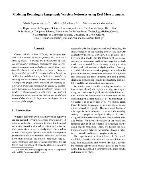
<strong>Model<strong>in</strong>g</strong> <strong>Roam<strong>in</strong>g</strong> <strong>in</strong> <strong>Large</strong>-<strong>scale</strong> <strong>Wireless</strong> <strong>Networks</strong> us<strong>in</strong>g <strong>Real</strong> Measurements<br />
Maria Papadopouli abc Michael Moudatsos bc Merkourios Karaliopoulos a<br />
a. Department of Computer Science, University of North Carol<strong>in</strong>a at Chapel Hill, USA.<br />
b. Institute of Computer Science, Foundation for Research and Technology-Hellas, Greece.<br />
c. Department of Computer Science, University of Crete, Greece.<br />
Emails: fmaria,mkaraliog@cs.unc.edu, moudatso@ics.forth.gr<br />
Abstract<br />
Campus wireless LANs (WLANs) are complex systems<br />
with hundreds of access po<strong>in</strong>ts (APs) and thousands<br />
of users. To analyze the performance of wireless<br />
network<strong>in</strong>g protocols, researchers need to construct<br />
simulations and testbed experiments that reproduce<br />
the characteristics of these networks. However,<br />
the generation of realistic models and benchmarks is<br />
challeng<strong>in</strong>g and there is only a limited set of models of<br />
roam<strong>in</strong>g and access based on real measurement data.<br />
We employed graph theory, modeled the roam<strong>in</strong>g activity<br />
as a graph and measured its degree of connectivity.<br />
The Negative B<strong>in</strong>omial distribution models well<br />
the degree of connectivity. Furthermore, we analyzed<br />
the evolution of the roam<strong>in</strong>g activity <strong>in</strong> the spatial and<br />
temporal doma<strong>in</strong> and its impact on the degree of connectivity<br />
of the graph.<br />
1 Introduction<br />
<strong>Wireless</strong> networks are <strong>in</strong>creas<strong>in</strong>gly be<strong>in</strong>g deployed<br />
and the demand for wireless access grows rapidly. It<br />
becomes particularly <strong>in</strong>trigu<strong>in</strong>g to study the temporal<br />
and spatial evolution of wireless networks. Unlike the<br />
wired networks that are relatively fixed, the wireless<br />
networks are highly dynamic due to the radio propagation<br />
effects and user mobility. <strong>Wireless</strong> LANs have<br />
more vulnerabilities and stricter bandwidth and latency<br />
constra<strong>in</strong>ts than their wired counterparts. For the<br />
design and evaluation of capacity plann<strong>in</strong>g, resource<br />
This work was partially supported by the IBM Corporation<br />
under an IBM Faculty Award 2005 grant.<br />
reservation, device adaptation, and load balanc<strong>in</strong>g, the<br />
characterization of the roam<strong>in</strong>g activity and <strong>in</strong>ter-AP<br />
connectivity is critical. Currently, there is lack of publicly<br />
available models for the topology of large-<strong>scale</strong><br />
wireless <strong>in</strong>frastructures and their access patterns. Such<br />
models are essential for perform<strong>in</strong>g mean<strong>in</strong>gful simulation<br />
and performance analysis studies. Contrary<br />
to traditional wired-network topologies that reflect the<br />
physical hardwired connection of routers or AS, wireless<br />
topologies are more dynamic and have a strong<br />
stochastic element due to radio propagation, user mobility<br />
and the AP association mechanisms.<br />
We aim to characterize the roam<strong>in</strong>g <strong>in</strong> a wireless <strong>in</strong>frastructure,<br />
identify the regions with high roam<strong>in</strong>g activity,<br />
and derive topological models of the <strong>in</strong>frastructure.<br />
Unlike our earlier research efforts that focused<br />
on roam<strong>in</strong>g on a client basis [15, 14, 5], this paper <strong>in</strong>vestigates<br />
it <strong>in</strong> an aggregate level. We employ graph<br />
theory to model the roam<strong>in</strong>g of wireless clients dur<strong>in</strong>g<br />
a time <strong>in</strong>terval as a graph. The ma<strong>in</strong> contribution of<br />
this paper is methodological. It models the roam<strong>in</strong>g<br />
activity as a graph and analyzes its degree of connectivity,<br />
which is modeled well by the Negative B<strong>in</strong>omial<br />
distribution. We discuss the impact of the spatial and<br />
temporal growth of the wireless <strong>in</strong>frastructure on the<br />
graph and its properties. Also, we discuss the nonl<strong>in</strong>ear<br />
correlation between the number of roam<strong>in</strong>gs between<br />
two APs and their geographic distance.<br />
The paper is structured as follows. In Section 2,<br />
we briefly describe the wireless network <strong>in</strong>frastructure,<br />
data acquisition, and testbed. Section 3 models<br />
the roam<strong>in</strong>g activity and Section 4 presents the related<br />
work. F<strong>in</strong>ally, Section 5 summarizes the ma<strong>in</strong> results<br />
and future work plans.
Table 1. Number of clients and APs dur<strong>in</strong>g the<br />
trac<strong>in</strong>g periods<br />
Week Trac<strong>in</strong>g Period Clients Total APs<br />
1 17-24, October 2004 8880 459<br />
2 2-9, March 2005 9049 532<br />
3 13-20, April 2005 9881 574<br />
2 <strong>Large</strong>-<strong>scale</strong> wireless network testbed and<br />
data acquisition<br />
The IEEE 802.11 <strong>in</strong>frastructure at the University<br />
of North Carol<strong>in</strong>a at Chapel Hill provides coverage<br />
for the 729-acre campus and a number of off-campus<br />
adm<strong>in</strong>istrative offices. The network APs belong to<br />
three different series of the Cisco Aironet platform: the<br />
state-of-the-art 1200 Series (269 APs), the widely deployed<br />
350 Series (188 APs) and the older 340 Series<br />
(31 APs). The 1200s and 350s come with Cisco IOS,<br />
while the 340s run VxWorks. The campus APs were<br />
configured to send syslog messages to a syslog server<br />
<strong>in</strong> our department. An AP generates syslog messages<br />
for IEEE 802.11 MAC events, <strong>in</strong>dicat<strong>in</strong>g when a user<br />
associates or disassociates, authenticates or deauthenticates<br />
with an AP, or roams from and to another AP. In<br />
our earlier work [5], we describe <strong>in</strong> detail how clients<br />
communicate with APs, the events that allow us to log<br />
the clients’ activities, and the measures taken to ensure<br />
users’ privacy while acquir<strong>in</strong>g and process<strong>in</strong>g the<br />
traces. While there is a small percentage of PDAs,<br />
the majority of the devices are laptops. In addition to<br />
each AP’s unique IP address, we ma<strong>in</strong>ta<strong>in</strong> <strong>in</strong>formation<br />
about the build<strong>in</strong>gs where APs are located <strong>in</strong> and their<br />
2D coord<strong>in</strong>ates.<br />
We acquire and analyze syslog data from three different<br />
monitor<strong>in</strong>g periods cover<strong>in</strong>g the <strong>in</strong>terval from<br />
October 2004 to April 2005. Table 1 describes the evolution<br />
of the wireless <strong>in</strong>frastructure across each period.<br />
The <strong>in</strong>crease of APs and WLAN clients is significant<br />
not only between the first and second trac<strong>in</strong>g period,<br />
but also with<strong>in</strong> the month separat<strong>in</strong>g the second from<br />
the third trac<strong>in</strong>g period. Such analysis allows track<strong>in</strong>g<br />
the temporal evolution of the wireless network and<br />
draw<strong>in</strong>g h<strong>in</strong>ts for time-persistent features.<br />
3 <strong>Model<strong>in</strong>g</strong> roam<strong>in</strong>g activity as graph<br />
We model the roam<strong>in</strong>g of clients with<strong>in</strong> the campus<br />
wireless network dur<strong>in</strong>g a trac<strong>in</strong>g period T as a graph<br />
G T =(V T E T ). Each AP deployed <strong>in</strong> the <strong>in</strong>frastructure<br />
corresponds to a node of the graph. We create<br />
an edge from node i to node j, if at least one client<br />
transition from AP i to AP j was recorded dur<strong>in</strong>g the<br />
trac<strong>in</strong>g period T . There is a transition from AP i to AP<br />
j, if there is a roam<strong>in</strong>g syslog message from AP i and<br />
a reassociation message from AP j, without any disassociation<br />
message from AP j at the same time. All<br />
these syslog messages for build<strong>in</strong>g a transition should<br />
come from the same client. These transitions are based<br />
on the syslog messages generated by APs upon IEEE<br />
802.11 MAC-level events as described <strong>in</strong> Section 2.<br />
The weight of an edge <strong>in</strong>dicates the total number of<br />
transitions between the correspond<strong>in</strong>g APs and its distance<br />
the geographic distance of the build<strong>in</strong>gs where<br />
the correspond<strong>in</strong>g APs are located. To construct the<br />
graph, we consider all clients’ transitions. We call<br />
these graphs roam<strong>in</strong>g graphs.<br />
A transition occurs due to either actual user mobility<br />
or changes <strong>in</strong> signal strength that affect the association.<br />
In [14], we found that 24% of the clients were<br />
mobile <strong>in</strong> terms of <strong>in</strong>ter-build<strong>in</strong>g AP transitions. Typically,<br />
a client selects to associate with the AP from<br />
which it receives stronger signal. When the signal<br />
strength drops below a threshold, the client may scan<br />
the channels and select the AP from which it receives<br />
the strongest signal. <strong>Wireless</strong> networks are highly dynamic<br />
environments and clients may experience several<br />
rapid “oscillations” between APs. Such oscillations<br />
due to radio propagation are very transient and<br />
do not reflect typical roam<strong>in</strong>g activity. To dist<strong>in</strong>guish<br />
them, we def<strong>in</strong>e the wiggl<strong>in</strong>g, as the case <strong>in</strong> which a<br />
client that was associated with an AP, gets associated<br />
briefly (i.e., for less than one second) with another AP,<br />
and then moves back to the first one.<br />
3.1 Degree of connectivity<br />
Figure 1 illustrates the quantile-quantile (qq) plots<br />
of the measured outdegrees for week 1 aga<strong>in</strong>st large<br />
samples drawn from four different discrete distributions,<br />
parameterized so that their mean is equal to the<br />
measured outdegree mean. The qq plot is a graphical
30<br />
Q−Q plot data vs Neg B<strong>in</strong>omial samples<br />
80<br />
Q−Q plot data vs Geometric samples<br />
25<br />
60<br />
20<br />
40<br />
15<br />
20<br />
10<br />
5<br />
0<br />
0<br />
−20<br />
0 10 20 30 40 0 10 20 30 40<br />
Q−Q plot data vs B<strong>in</strong>omial samples<br />
Q−Q plot data vs Poisson samples<br />
20<br />
20<br />
15<br />
15<br />
Density<br />
0.12<br />
0.1<br />
0.08<br />
0.06<br />
Histogram of real data<br />
Negative B<strong>in</strong>omial<br />
10<br />
10<br />
0.04<br />
5<br />
0<br />
0 10 20 30 40<br />
5<br />
0<br />
0 10 20 30 40<br />
Figure 1. Q-Q plots of AP outdegree aga<strong>in</strong>st<br />
four discrete distributions (week 1)<br />
0.02<br />
0<br />
0 5 10 15 20 25 30<br />
Degree of connectivity<br />
Figure 2. Histogram of data and Negative B<strong>in</strong>omial<br />
theoretical mass function<br />
technique for determ<strong>in</strong><strong>in</strong>g if two data sets come from<br />
populations with a common distribution. The graphical<br />
tests suggest that both the Geometric and Negative<br />
B<strong>in</strong>omial distributions are possible matches for<br />
the degree of connectivity distribution with the l<strong>in</strong>ear<br />
regression yield<strong>in</strong>g correlation coeffiecient values <strong>in</strong><br />
the order of 0.95-0.98 for all trac<strong>in</strong>g periods and <strong>in</strong>degree<br />
and outdegree of connectivity. Nevertheless,<br />
the hypothesis that the degree of connectivity follows<br />
the Geometric distribution is rejected by the chi-square<br />
test, even at the 10% level of significance. On the<br />
contrary, the Negative B<strong>in</strong>omial distribution passes the<br />
test at 1% significance level for all traces, reveal<strong>in</strong>g a<br />
time-persistent feature <strong>in</strong> the <strong>in</strong>frastructure connectivity.<br />
Notably, the specific hypothesis passes also the<br />
Kolmogorov-Smirnov statistic [16] for discrete data,<br />
which normally yields more extreme values from the<br />
Pearson chi-square statistic [6]. The histogram of the<br />
degree of connectivity is plotted aga<strong>in</strong>st the theoretical<br />
distribution with Maximum Likelihood (ML) estimates<br />
for its parameters r and p <strong>in</strong> Figure 2, whereas<br />
Table 2 reports the ML estimates for the Negative B<strong>in</strong>omial<br />
distribution parameters. Faloutsos et al. [7]<br />
argue <strong>in</strong> favor of a power-law relationship between the<br />
degree of connectivity and its frequency for the Internet<br />
topology at the network doma<strong>in</strong> connectivity level.<br />
Compared to the Internet topology, a campus WLAN<br />
exhibits a flatter connectivity structure. In the loglog<br />
<strong>scale</strong> plots of the outdegree frequency versus the<br />
Table 2. ML estimates for the Negative B<strong>in</strong>omial<br />
parameters<br />
Edges Week 1 Week 2 Week 3<br />
Incom<strong>in</strong>g 1.51, 0.21 1.78, 0.26 1.83, 0.25<br />
Outgo<strong>in</strong>g 1.58, 0.22 1.79, 0.26 1.73, 0.23<br />
Fraction of nodes with more than x total edges<br />
1<br />
0.9<br />
0.8<br />
0.7<br />
0.6<br />
0.5<br />
0.4<br />
0.3<br />
0.2<br />
0.1<br />
week 1<br />
week 2<br />
week 2<br />
0<br />
0 10 20 30 40 50 60 70<br />
Number of total edges<br />
Figure 3. Degree of connectivity
outdegree (Figure 3 [13]), the correlation coefficient<br />
ranges from 0.88 to 0.91.<br />
Figure 3 shows the CCDF of the degree of connectivity<br />
for the three trac<strong>in</strong>g periods (namely, weeks 1,<br />
2, and 3). The stochastic order of nodes with small<br />
or medium degree of connectivity is different from the<br />
one of nodes with high degree of connectivity over the<br />
three weeks. Up to a certa<strong>in</strong> degree of connectivity<br />
value (18), the last week has the highest degree <strong>in</strong> the<br />
stochastic order among the three weeks. Beyond this<br />
value (<strong>in</strong>dicated by a black vertical l<strong>in</strong>e <strong>in</strong> Figure 3),<br />
the stochastic order changes. Let us def<strong>in</strong>e as crosspo<strong>in</strong>ts<br />
the nodes with a degree of connectivity greater<br />
than 18 and focus more on the distribution of these<br />
nodes. A crosspo<strong>in</strong>t corresponds to an AP that received<br />
or sent a number of roam<strong>in</strong>g clients from (to)<br />
a relative large number of neighbor<strong>in</strong>g APs. We will<br />
refer to that AP as crosspo<strong>in</strong>t AP. Essentially, crosspo<strong>in</strong>t<br />
APs identify regions with high roam<strong>in</strong>g activity.<br />
In week 1, the percentage of crosspo<strong>in</strong>ts (14%) is<br />
greater than that of weeks 2 and 3 (13% and 10%, respectively).<br />
Furthermore, there is a 40% <strong>in</strong>crease <strong>in</strong><br />
the number of crosspo<strong>in</strong>ts from week 2 to week 3.<br />
How does the <strong>in</strong>frastructure evolve and what is its<br />
impact on the properties of the graph? Where are the<br />
new APs be<strong>in</strong>g placed? New APs were added, aim<strong>in</strong>g<br />
to extend or enhance the wireless coverage by offer<strong>in</strong>g<br />
better signal strength to more clients. There was<br />
a 16% and 8% <strong>in</strong>crease <strong>in</strong> the number of APs dur<strong>in</strong>g<br />
the second and third week, respectively. A newly<br />
added AP could be placed <strong>in</strong> either an isolated area or<br />
close to other APs. Isolated APs contribute with nodes<br />
with a small degree of connectivity. Table 3 summarizes<br />
the growth of the <strong>in</strong>frastructure <strong>in</strong> terms of number<br />
of APs with high roam<strong>in</strong>g activity. The “Common<br />
to prior week” <strong>in</strong>dicates the number of APs that<br />
were crosspo<strong>in</strong>ts <strong>in</strong> both current and previous trac<strong>in</strong>g<br />
period, “Common <strong>in</strong> all weeks” the number of APs<br />
which were crosspo<strong>in</strong>ts <strong>in</strong> all three weeks, and “Common<br />
<strong>in</strong> any week” the number of crosspo<strong>in</strong>ts of the<br />
current week which were also crosspo<strong>in</strong>ts <strong>in</strong> any of<br />
the other two weeks. The total number of crosspo<strong>in</strong>ts<br />
falls slightly (9%) from week 1 to week 2, before it<br />
rises <strong>in</strong> week 3. This fall can be caused due to either<br />
reduced user mobility or placement of new APs. S<strong>in</strong>ce<br />
the 20% of crosspo<strong>in</strong>ts of week 2 and 30% of week<br />
3 were newly added APs with respect to prior weeks,<br />
we speculate that they were placed <strong>in</strong> popular areas<br />
with extensive roam<strong>in</strong>g activity. The placement of new<br />
APs <strong>in</strong> proximity to other APs can only partially alleviate<br />
the wiggl<strong>in</strong>gs, s<strong>in</strong>ce they may <strong>in</strong>troduce new<br />
ones. This was apparent <strong>in</strong> our <strong>in</strong>frastructure. Specifically,<br />
56% of the common APs <strong>in</strong> all three trac<strong>in</strong>g periods<br />
experience an <strong>in</strong>crease <strong>in</strong> the number of wiggl<strong>in</strong>gs<br />
(median rise of 2), whereas the rema<strong>in</strong><strong>in</strong>g APs had a<br />
decrease (median fall of 4.5 <strong>in</strong>clud<strong>in</strong>g those with fall<br />
equal to 0, from week 1 to week 2). From week 2 to<br />
week 3, a 21% of APs had an <strong>in</strong>crease <strong>in</strong> their number<br />
of wiggl<strong>in</strong>gs by a median rise of 5 and the rema<strong>in</strong><strong>in</strong>g<br />
had a median fall of 3.<br />
Figure 4 illustrates the graph evolution through the<br />
three trac<strong>in</strong>g periods and its spatial characteristics.<br />
Each po<strong>in</strong>t <strong>in</strong> the plot represents all APs located <strong>in</strong> the<br />
build<strong>in</strong>g (with the same coord<strong>in</strong>ates as the po<strong>in</strong>t). Consequently,<br />
edges between APs <strong>in</strong> the same build<strong>in</strong>g or<br />
edges between APs <strong>in</strong> different build<strong>in</strong>gs are overlapp<strong>in</strong>g<br />
with each other and are not dist<strong>in</strong>guishable <strong>in</strong> that<br />
plot. Arround the periphery of the campus, we can dist<strong>in</strong>guish<br />
new isolated nodes with low degree of connectivity.<br />
While <strong>in</strong> more dense areas, the newly placed<br />
APs and their neighbors exhibit a relatively high degree<br />
of connectivity.<br />
3.2 Degree of connectivity vs. distance<br />
We expected to f<strong>in</strong>d a relation between the number<br />
of transitions between two APs and their distance. In<br />
[13], a scatterplot illustrates the number of transitions<br />
between APs versus their Euclidean distance. In this<br />
analysis, we only consider pairs of APs with at least<br />
one transition. The Pearson product-moment correlation<br />
coefficient R of these two variables ranges from -<br />
0.04 to -0.09 for the the three trac<strong>in</strong>g periods. The low<br />
values of R imply that the correlation under discussion<br />
has non-l<strong>in</strong>ear characteristics, although they are<br />
still high enough to reject the null hypothesis of no dependence<br />
between the two data sets at 1% significance<br />
level. We computed the Spearman rank correlation coefficient<br />
[11], a non-parametric statistic that does not<br />
make any assumption about the underly<strong>in</strong>g distribution<br />
of the analyzed data. These values ranged from<br />
-0.29 (week 3) to -0.45 (week 1). In all cases the null<br />
hypothesis that the two variables are <strong>in</strong>dependent is rejected<br />
at significance levels far beyond 1%. Further
Table 3. Evolution of crosspo<strong>in</strong>ts <strong>in</strong> the graph dur<strong>in</strong>g the trac<strong>in</strong>g periods<br />
Week Total nodes Crosspo<strong>in</strong>ts Common to prior week Common <strong>in</strong> all weeks Common <strong>in</strong> any week<br />
1 459 71 0 51 55<br />
2 532 65 52 51 62<br />
3 574 91 61 51 64<br />
7.9 x 10⁵ x coord<strong>in</strong>ate<br />
7.9 x 10⁵ x coord<strong>in</strong>ate<br />
7.9 x 10⁵ x coord<strong>in</strong>ate<br />
7.89<br />
week 1<br />
7.89<br />
week 2<br />
7.89<br />
week 3<br />
7.88<br />
7.88<br />
7.88<br />
x coord<strong>in</strong>ate<br />
7.87<br />
7.86<br />
7.85<br />
y coord<strong>in</strong>ate<br />
7.87<br />
7.86<br />
7.85<br />
y coord<strong>in</strong>ate<br />
7.87<br />
7.86<br />
7.85<br />
7.84<br />
7.84<br />
7.84<br />
7.83<br />
7.83<br />
7.83<br />
7.82<br />
1.981 1.982 1.983 1.984 1.985 1.986 1.987 1.988 1.989<br />
7.82<br />
1.981 1.982 1.983 1.984 1.985 1.986 1.987 1.988 1.989<br />
7.82<br />
1.981 1.982 1.983 1.984 1.985 1.986 1.987 1.988 1.989<br />
Figure 4. Transition graph <strong>in</strong> three week periods<br />
support<strong>in</strong>g evidence for the existence of negative correlation<br />
between the distance of two APs and the number<br />
of transitions measured from the one to the other,<br />
came from the test of <strong>in</strong>dependence <strong>in</strong> cont<strong>in</strong>gency tables<br />
[17]. The computed values of the statistics are<br />
four (week 2) to seven (week 1) times the critical values<br />
at the 1% significance level, reject<strong>in</strong>g strongly the<br />
null hypothesis for <strong>in</strong>dependence of the two data sets.<br />
4 Related Work<br />
Albert and Barabasi [1] focus on the statistical mechanics<br />
of network topology and dynamics, the ma<strong>in</strong><br />
models and analytical tools for random graphs, smallworld<br />
and <strong>scale</strong>-free networks, the emerg<strong>in</strong>g theory of<br />
evolv<strong>in</strong>g networks, and the <strong>in</strong>terplay between topology<br />
and the networks robustness aga<strong>in</strong>st failures and attacks.<br />
Faloutsos et al. [7] prove that the AS and router<br />
level <strong>in</strong>ternet topology can be described with power<br />
laws. Lun Li et al. [12] propose a complementary<br />
approach of model<strong>in</strong>g <strong>in</strong>ternet’s router-level topology.<br />
They characterise current degree-based approaches as<br />
<strong>in</strong>complete s<strong>in</strong>ce graphs with the same node degree<br />
distribution can result from different graphs <strong>in</strong> terms<br />
of network eng<strong>in</strong>eer<strong>in</strong>g. Borrel et al. [4] form a new<br />
mobility model that <strong>in</strong>corporates <strong>in</strong>dividual behavior<br />
and group <strong>in</strong>teraction based on the preferential attachment<br />
pr<strong>in</strong>ciple. Their simulations yielded topologies<br />
with <strong>scale</strong>-free spatial distribution of nodes.<br />
This research extends our earlier studies [5], [14],<br />
[15], the studies by Henderson et al. [8], Kotz and<br />
Essien [10], Balachandran et al. [2] and Balaz<strong>in</strong>ska<br />
and Castro [3] by focus<strong>in</strong>g more closely on the<br />
roam<strong>in</strong>g activity <strong>in</strong> an aggregate level and the APtopological<br />
properties. In [15], we modeled the arrival<br />
of wireless clients at the access po<strong>in</strong>ts (APs) <strong>in</strong><br />
a production 802.11 <strong>in</strong>frastructure as a time-vary<strong>in</strong>g<br />
Poisson processes. These results were validated us<strong>in</strong>g<br />
quantile plots with simulation envelope for goodnessof-fit<br />
tests and by model<strong>in</strong>g the visit arrivals at different<br />
time <strong>in</strong>tervals and APs. M<strong>in</strong>kyong et al. [9] cluster<br />
APs based on their peak hours and analyze the distribution<br />
of arrivals for each cluster, us<strong>in</strong>g the aggregate<br />
client arrivals and departures at APs. Our earlier work<br />
[5] models the associations of each wireless client as<br />
a Markov-cha<strong>in</strong> <strong>in</strong> which a state corresponds to an AP<br />
that the client has visited. Based on the history of transitions<br />
between APs, we build a Markov-cha<strong>in</strong> model<br />
for each client. Even for the very mobile clients, this<br />
model can predict well the next AP that a client will<br />
visit while roam<strong>in</strong>g <strong>in</strong> the wireless <strong>in</strong>frastructure. Furthermore,<br />
a class of bipareto distributions can be employed<br />
to model the duration of visits at APs and cont<strong>in</strong>uous<br />
wireless access [14].
5 Conclusions and future work<br />
We modeled the roam<strong>in</strong>g activity as a graph and<br />
measured its properties and evolution <strong>in</strong> the spatial and<br />
temporal doma<strong>in</strong>. For example, the degree of connectivity<br />
can be modeled us<strong>in</strong>g a Negative B<strong>in</strong>omial<br />
distribution. The placement of new APs results <strong>in</strong> a<br />
decrease of the percentage of crosspo<strong>in</strong>t APs. Furthermore,<br />
a large percentage of APs are placed <strong>in</strong> the vic<strong>in</strong>ity<br />
of APs with high roam<strong>in</strong>g patterns. We evaluated<br />
the impact of newly added APs on the degree of connectivity.<br />
A natural extension of this paper is the detection<br />
and model<strong>in</strong>g of the weak spots <strong>in</strong> a wireless network,<br />
through complementary graphs where an edge represents<br />
unsuccessful roam<strong>in</strong>g transitions. Such graphs<br />
could be employed as diagnostic tools by reveal<strong>in</strong>g<br />
problems, such as misconfigured or misplaced APs.<br />
It would be <strong>in</strong>terest<strong>in</strong>g to validate and contrast such<br />
results with tools based on signal strength <strong>in</strong>formation.<br />
The acquisition of signal strength measurements<br />
<strong>in</strong> large-<strong>scale</strong>, uncontrolled environments is challeng<strong>in</strong>g<br />
and the use of cross-layer <strong>in</strong>formation <strong>in</strong> larger<br />
time <strong>scale</strong>s can be helpful. F<strong>in</strong>ally, we plan to analyze<br />
traces from different wireless environments, contrast<br />
their correspond<strong>in</strong>g graphs, and evaluate the impact of<br />
the network size, AP density, and access pattern on the<br />
graph.<br />
References<br />
[1] R. Albert and A.-L. Barabasi. Statistical mechanics<br />
of complex networks. In Rev. of Modern Physics,volume<br />
74, 2002.<br />
[2] A. Balachandran, G. Voelker, P. Bahl, and V. Rangan.<br />
Characteriz<strong>in</strong>g user behavior and network performance<br />
<strong>in</strong> a public wireless lan. In Proceed<strong>in</strong>gs<br />
of the ACM Sigmetrics Conference on Measurement<br />
and <strong>Model<strong>in</strong>g</strong> of Computer Systems, California, USA,<br />
2002.<br />
[3] M. Balaz<strong>in</strong>ska and P. Castro. Characteriz<strong>in</strong>g mobility<br />
and network usage <strong>in</strong> a corporate wireless local-area<br />
network. In First International Conference on Mobile<br />
Systems, Applications, and Services (MobiSys), San<br />
Francisco, USA, May 2003.<br />
[4] V. Borrel, M. D. de Amorim, and S. Fdida. On natural<br />
mobility models. In LNCS, International Workshop<br />
on Autonomic Communication (WAC), Athens,<br />
Greece, October 2005.<br />
[5] F. Ch<strong>in</strong>chilla, M. L<strong>in</strong>dsey, and M. Papadopouli. Analysis<br />
of wireless <strong>in</strong>formation locality and association<br />
patterns <strong>in</strong> a campus. In Proceed<strong>in</strong>gs of the IEEE<br />
Conference on Computer Communications (Infocom),<br />
Hong Kong, March 2004.<br />
[6] R. B. D’Agost<strong>in</strong>o and M. A. Stephens. Goodness-offit<br />
techniques. Statistics: Textbooks and Monographs,<br />
New York: Dekker, 1986, edited by D’Agost<strong>in</strong>o,<br />
Ralph B.; Stephens, Michael A., 1986.<br />
[7] M. Faloutsos, P. Faloutsos, and C. Faloutsos. On<br />
power-law relationships of the <strong>in</strong>ternet topology.<br />
In SIGCOMM Symposium on Communications Architectures<br />
and Protocols, Philadelphia, September<br />
1999.<br />
[8] T. Henderson, D. Kotz, and I. Abyzov. The chang<strong>in</strong>g<br />
usage of a mature campuswide wireless network. In<br />
ACM International Conference on Mobile Comput<strong>in</strong>g<br />
and Network<strong>in</strong>g (MobiCom), Philadelphia, September<br />
2004.<br />
[9] M. Kim and D. Kotz. <strong>Model<strong>in</strong>g</strong> users’ mobility<br />
among wifi access po<strong>in</strong>ts. In WiTMeMo ’05, Berkeley,<br />
CA, USA, June 2005. USENIX Association.<br />
[10] D. Kotz and K. Essien. Analysis of a campuswide<br />
wireless network. Technical Report TR2002-<br />
432, Dept. of Computer Science, Dartmouth College,<br />
September 2002.<br />
[11] E. L. Lehmann and H. J. M. D’Abrera. Nonparametrics:<br />
Statistical Methods Based on Ranks, rev. ed.<br />
Prentice-Hall, New Jersey, NJ, USA, 1998.<br />
[12] L. Li, D. Alderson, W. Will<strong>in</strong>ger, and J. Doyle. A<br />
first pr<strong>in</strong>ciples approach to understand<strong>in</strong>g the <strong>in</strong>ternet’s<br />
router-level topology. In ACM SIGCOMM,<br />
Philadelpia, USA, 2004.<br />
[13] M. Papadopouli, M. Moudatsos, and M. Karaliopoulos.<br />
<strong>Model<strong>in</strong>g</strong> roam<strong>in</strong>g <strong>in</strong> large-<strong>scale</strong> wireless networks<br />
us<strong>in</strong>g real measurements. Technical Report<br />
369, ICS-FORTH, Greece, January 2006.<br />
[14] M. Papadopouli, H. Shen, and M. Spanakis. Characteriz<strong>in</strong>g<br />
the duration and association patterns of wireless<br />
access <strong>in</strong> a campus. In 11th European <strong>Wireless</strong><br />
Conference, Nicosia, Cyprus, April 2005.<br />
[15] M. Papadopouli, H. Shen, and M. Spanakis. <strong>Model<strong>in</strong>g</strong><br />
client arrivals at access po<strong>in</strong>ts <strong>in</strong> wireless campuswide<br />
networks. In 14th IEEE Workshop on Local<br />
and Metropolitan Area <strong>Networks</strong>, Chania, Greece,<br />
September 2005.<br />
[16] A. Pettitt and M. A. Stephens. The kolmogorovsmirnov<br />
goodness-of-fit test for discrete and grouped<br />
data. In Technometrics, volume 19, pages 205–210,<br />
May 1977.<br />
[17] S. Ross. Introduction to probability and statistics for<br />
eng<strong>in</strong>eers and scientists. Wiley Series <strong>in</strong> Probability<br />
and mathematical statistics, 1987.